Probabilistic Parsing Strategies

Context-free grammars and push-down automata are two equivalent formalisms to describe context-free languages. While a context-free grammar can be thought of as a purely declarative specification, a push-down automaton is considered to be an operational specification that determines which steps are performed for a given string in the process of deciding its membership of the language. By a parsing strategy we mean a mapping from context-free grammars to equivalent push-down automata, such that some specific conditions are observed.

This paper deals with the probabilistic extensions of context-free grammars and push-down automata, i.e., probabilistic context-free grammars [36, 4] and probabilistic push-down automata [36, 37, 45, 1]. These formalisms are obtained by adding probabilities to the rules and transitions of context-free grammars and push-down automata, respectively. More specifically, we will investigate the problem of ‘extending’ parsing strategies to probabilistic parsing strategies. These are mappings from probabilistic context-free grammars to probabilistic push-down automata that preserve the induced probability distributions on the generated/accepted languages. Two of the main results presented in this paper can be stated as follows:

• •

  No parsing strategy that lacks the correct-prefix property (CPP) can be extended to become a probabilistic parsing strategy.

• •

  All parsing strategies that possess the correct-prefix property and the strong predictiveness property (SPP) can be extended to become probabilistic parsing strategies.

The above results generalize previous findings reported in [45, 46, 1], where only a few specific parsing strategies were considered in isolation. Our findings also have important implications for well-known parsing strategies such as generalized LR parsing, henceforth simply called ‘LR parsing’.¹¹ 1 Generalized (or nondeterministic) LR parsing allows for more than one action for a given LR state and input symbol. LR parsing has the CPP, but lacks the SPP, and as we will show, LR parsing cannot be extended to become a probabilistic parsing strategy.

In the last decade, widespread interest in probabilistic parsing techniques has arisen in the area of natural language processing [6, 25, 20]. This is motivated by the fact that natural language sentences are generally ambiguous, and natural language software needs to be able to distinguish the more probable derivations of a sentence from the less probable ones. This can be achieved by letting the parsing process assign a probability to each parse, on the basis of a probabilistic grammar. In a typical application, the software may select those derivations for further processing that have been given the highest probabilities, and discard the others. The success of this approach relies on the accuracy of the probabilistic model expressed by the probabilistic grammar, i.e., whether the probabilities assigned to derivations accurately reflect the ‘true’ probabilities in the domain at hand.

Probabilities are often estimated on the basis of a corpus, i.e., a collection of sentences. The sentences in a corpus may be annotated with various kinds of information. One kind of annotation that is relevant for our discussion is the preferred derivation for each sentence. Given a corpus with derivations, one may estimate probabilities of rules by their relative frequencies in the corpus. If a corpus is unannotated, more general techniques of maximum-likelihood estimation can be used to estimate the probabilities of rules. (See [35, 11, 10] for some formal properties of types of maximum-likelihood estimation.)

The motivation for studying probabilistic models other than those obtained by attaching probabilities to given context-free grammars is the observation that more accurate models can be obtained by conditioning probabilities on ‘context information’ beyond single nonterminals [12, 8]. Furthermore, it has been observed that conditioning on certain types of context information can be achieved by first translating context-free grammars to push-down automata, according to some parsing strategy, and then attaching probabilities to the transitions thereof [43, 33]. More concretely, for some parsing strategies, the set of models that can be obtained by attaching probabilities to a push-down automaton constructed from a context-free grammar may include models that cannot be obtained by attaching probabilities to that grammar.

An implicit assumption of this methodology is that, conversely, any probabilistic model that can be obtained from a grammar can also be obtained from the associated push-down automaton, or in other words, the push-down automaton is at least as powerful as the grammar in terms of the set the potential models. If a parsing strategy does not satisfy this property, and if some potential models are lost in the mapping from the grammar to the push-down automaton, then this means that in some cases the strategy may lead to less rather than more accurate models. That LR parsing cannot be extended to become a probabilistic parsing strategy, as we mentioned above, means that the above property is not satisfied by this parsing strategy. This is contrary to what is suggested by some publications on probabilistic LR parsing, such as [5] and [18], which fail to observe that LR parsers may sometimes lead to less accurate models than the grammars from which they were constructed.

Some studies, such as [13, 9, 7], propose lexicalized probabilistic context-free grammars, i.e., probabilistic models based on context-free grammars in which probabilities heavily rely on the terminal elements from input strings. Even if the current paper does not specifically deal with lexicalization, much of what we discuss pertains to lexicalized probabilistic context-free grammars as well.

The paper is organized as follows. After giving standard definitions in Section 2, we give our formal definition of ‘parsing strategy’ in Section 3. We also define what it means to extend a parsing strategy to become a probabilistic parsing strategy. The CPP and the SPP are defined in Sections 4 and 5, where we also discuss how these properties relate to the question of which strategies can be extended to become probabilistic. Sections 6 and 7 provide examples of parsing strategies with and without the SPP. The examples without the SPP, most notably LR parsing, are shown not to be extendible to become probabilistic. A wider notion of extending a strategy to become probabilistic is provided by Section 8. We show that even under this wider notion, LR parsing cannot be extended to become probabilistic. Section 9 presents an application that concerns prefix probabilities. We end this paper with conclusions.

Some results reported here have appeared before in an abbreviated form in [29].

A context-free grammar (CFG) ${\cal G}$ is a 4-tuple $(\Sigma,$ $N,$ $S,$ $R)$, where $\Sigma$ is a finite set of terminals, called the alphabet, $N$ is a finite set of nonterminals, including the start symbol $S$, and $R$ is a finite set of rules, each of the form $A\rightarrow\alpha$, where $A\in N$ and $\alpha\in(\Sigma\cup N)^{\ast}$. Without loss of generality, we assume that there is only one rule $S\rightarrow\sigma$ with the start symbol in the left-hand side, and furthermore that $\sigma\neq\epsilon$, where $\epsilon$ denotes the empty string.

For a fixed CFG ${\cal G}$, we define the relation $\Rightarrow$ on triples consisting of two strings $\alpha,\beta\in(\Sigma\cup N)^{\ast}$ and a rule $\pi\in R$ by: $\alpha\stackrel{{\scriptstyle\pi}}{{\Rightarrow}}\beta$ if and only if $\alpha$ is of the form $wA\delta$ and $\beta$ is of the form $w\gamma\delta$, for some $w\in\Sigma^{\ast}$ and $\delta\in(\Sigma\cup N)^{\ast}$, and $\pi=(A\rightarrow\gamma)$. A left-most derivation is a string $d=\pi_{1}\cdots\pi_{m}$, $m\geq 0$, such that $S\stackrel{{\scriptstyle\pi_{1}}}{{\Rightarrow}}\cdots\stackrel{{\scriptstyle\pi_{m}}}{{\Rightarrow}}\alpha$, for some $\alpha\in(\Sigma\cup N)^{\ast}$. We will identify a left-most derivation with the sequence of strings over $\Sigma\cup N$ that arise in that derivation. In the remainder of this paper, we will let the term ‘derivation’ refer to ‘left-most derivation’, unless specified otherwise.

A derivation $d=\pi_{1}\cdots\pi_{m}$, $m\geq 0$, such that $S\stackrel{{\scriptstyle\pi_{1}}}{{\Rightarrow}}\cdots\stackrel{{\scriptstyle\pi_{m}}}{{\Rightarrow}}w$ where $w\in\Sigma^{\ast}$ will be called a complete derivation; we also say that $d$ is a derivation of $w$. By subderivation we mean a substring of a complete derivation of the form $d=\pi_{1}\cdots\pi_{m}$, $m\geq 0$, such that $A\stackrel{{\scriptstyle\pi_{1}}}{{\Rightarrow}}\cdots\stackrel{{\scriptstyle\pi_{m}}}{{\Rightarrow}}w$ for some $A$ and $w$.

We write $\alpha\Rightarrow^{\ast}\beta$ or $\alpha\Rightarrow^{+}\beta$ to denote the existence of a string $\pi_{1}\cdots\pi_{m}$ such that $\alpha\stackrel{{\scriptstyle\pi_{1}}}{{\Rightarrow}}\cdots\stackrel{{\scriptstyle\pi_{m}}}{{\Rightarrow}}\beta$, with $m\geq 0$ or $m>0$, respectively. We say a CFG is acyclic if $A\Rightarrow^{+}A$ does not hold for any $A\in N$.

For a CFG ${\cal G}$ we define the language $L({\cal G})$ it generates as the set of strings $w$ such that there is at least one derivation of $w$. We say a CFG is reduced if for each rule $\pi\in R$ there is a complete derivation in which it occurs.

A probabilistic context-free grammar (PCFG) is a pair $({\cal G},p)$ consisting of a CFG ${\cal G}=(\Sigma,$ $N,$ $S,$ $R)$ and a probability function $p$ from $R$ to real numbers in the interval $[0,1]$. We say a PCFG is proper if $\Sigma_{\pi=(A\rightarrow\gamma)\in R}\ p(\pi)=1$ for each $A\in N$.

For a PCFG $({\cal G},p)$, we define the probability $p(d)$ of a string $d=\pi_{1}\cdots\pi_{m}\in R^{\ast}$ as $\prod_{i=1}^{m}\ p(\pi_{i})$; we will in particular consider the probabilities of derivations $d$. The probability $p(w)$ of a string $w\in\Sigma^{\ast}$ as defined by $({\cal G},p)$ is the sum of the probabilities of all derivations of that string. We say a PCFG $({\cal G},p)$ is consistent if $\Sigma_{w\in\Sigma^{\ast}}\ p(w)=1$.

In this paper we will mainly consider push-down transducers rather than push-down automata. Push-down transducers not only compute derivations of the grammar while processing an input string, but they also explicitly produce output strings from which these derivations can be obtained. We use transducers for two reasons. First, constraints on the output strings allow us to restrict our attention to ‘reasonable’ parsing strategies. Those strategies that cannot be formalized within these constraints are unlikely to be of practical interest. Secondly, mappings from input strings to derivations, as those realized by push-down devices, turn out to be a very powerful abstraction and allow direct proofs of several general results.

Differently from many textbooks, our push-down devices do not possess states next to stack symbols. This is without loss of generality, since states can be encoded into the stack symbols, given the types of transition that we allow. Thus, a push-down transducer (PDT) ${\cal A}$ is a 6-tuple $(\Sigma_{1},$ $\Sigma_{2},$ $Q,$ $X_{\it init},$ $X_{\it final},$ $\Delta)$, where $\Sigma_{1}$ is the input alphabet, $\Sigma_{2}$ is the output alphabet, $Q$ is a finite set of stack symbols including the initial stack symbol $X_{\it init}$ and the final stack symbol $X_{\it final}$, and $\Delta$ is the set of transitions. Each transition can have one of the following three forms: ${X}\mapsto{XY}$ (a push transition), ${\it YX}\mapsto{Z}$ (a pop transition), or ${X}\stackrel{{\scriptstyle x,y}}{{\mapsto}}{Y}$ (a swap transition); here $X$, $Y$, $Z\in Q$, $x\in\Sigma_{1}\cup\{\epsilon\}$ and $y\in\Sigma_{2}^{\ast}$. Note that in our notation, stacks grow from left to right, i.e., the top-most stack symbol will be found at the right end.

Without loss of generality, we assume that any PDT is such that for a given stack symbol $X\neq X_{\it final}$, there are either one or more push transitions ${X}\mapsto{XY}$, or one or more pop transitions ${\it YX}\mapsto{Z}$, or one or more swap transitions ${X}\stackrel{{\scriptstyle x,y}}{{\mapsto}}{Y}$, but no combinations of different types of transition. If a PDT does not satisfy this normal form, it can easily be brought in this form by introducing for each stack symbol $X$ three new stack symbols $X_{\it push}$, $X_{\it pop}$ and $X_{\it swap}$ and new swap transitions ${X}\stackrel{{\scriptstyle\epsilon,\epsilon}}{{\mapsto}}{X_{\it push}}$, ${X}\stackrel{{\scriptstyle\epsilon,\epsilon}}{{\mapsto}}{X_{\it pop}}$ and ${X}\stackrel{{\scriptstyle\epsilon,\epsilon}}{{\mapsto}}{X_{\it swap}}$. In each existing transition that operates on top-of-stack $X$, we then replace $X$ by one from $X_{\it push}$, $X_{\it pop}$ or $X_{\it swap}$, depending on the type of that transition. We also assume that $X_{\it final}$ does not occur in the left-hand side of a transition, again without loss of generality.

A configuration of a PDT is a triple $(\alpha,w,v)$, where $\alpha\in Q^{\ast}$ is a stack, $w\in\Sigma_{1}^{\ast}$ is the remaining input, and $v\in\Sigma_{2}^{\ast}$ is the output generated so far. For a fixed PDT ${\cal A}$, we define the relation $\vdash$ on triples consisting of two configurations and a transition $\tau$ by: $(\gamma\alpha,xw,v)\stackrel{{\scriptstyle\tau}}{{\vdash}}(\gamma\beta,w,vy)$ if and only if $\tau$ is of the form ${\alpha}\mapsto{\beta}$, where $x=y=\epsilon$, or of the form ${\alpha}\stackrel{{\scriptstyle x,y}}{{\mapsto}}{\beta}$. A computation on an input string $w$ is a string $c=\tau_{1}\cdots\tau_{m}$, $m\geq 0$, such that $(X_{\it init},w,\epsilon)\stackrel{{\scriptstyle\tau_{1}}}{{\vdash}}\cdots\stackrel{{\scriptstyle\tau_{m}}}{{\vdash}}(\alpha,w^{\prime},v)$. A complete computation on a string $w$ is a computation with $w^{\prime}=\epsilon$ and $\alpha=X_{\it final}$. The string $v$ is called the output of the computation $c$, and is denoted by ${\it out}(c)$.

We will identify a computation with the sequence of configurations that arise in that computation, where the first configuration is determined by the context. We also write $(\alpha,w,v)\vdash^{\ast}(\beta,w^{\prime},v^{\prime})$ or $(\alpha,w,v)\stackrel{{\scriptstyle c}}{{\vdash^{\ast}}}(\beta,w^{\prime},v^{\prime})$, for $\alpha,\beta\in Q^{\ast}$, $w,w^{\prime}\in\Sigma_{1}^{\ast}$ and $v,v^{\prime}\in\Sigma_{2}^{\ast}$, to indicate that $(\beta,w^{\prime},v^{\prime})$ can be obtained from $(\alpha,w,v)$ by applying a sequence $c$ of zero or more transitions; we refer to such a sequence $c$ as a subcomputation. The function ${\it out}$ is extended to subcomputations in a natural way.

For a PDT ${\cal A}$, we define the language $L({\cal A})$ it accepts as the set of strings $w$ such that there is at least one complete computation on $w$. We say a PDT is reduced if each transition $\tau\in\Delta$ occurs in some complete computation.

A probabilistic push-down transducer (PPDT) is a pair $({\cal A},p)$ consisting of a PDT ${\cal A}$ and a probability function $p$ from the set $\Delta$ of transitions of ${\cal A}$ to real numbers in the interval $[0,1]$. We say a PPDT $({\cal A},p)$ is proper if

• •

  $\Sigma_{\tau=({X}\mapsto{XY})\in\Delta}\ p(\tau)=1$ for each $X\in Q$ such that there is at least one transition ${X}\mapsto{XY}$, $Y\in Q$;

• •

  $\Sigma_{\tau=({X}\stackrel{{\scriptstyle x,y}}{{\mapsto}}{Y})\in\Delta}\ p(\tau)=1$ for each $X\in Q$ such that there is at least one transition ${X}\stackrel{{\scriptstyle x,y}}{{\mapsto}}{Y}$, $x\in\Sigma_{1}\cup\{\epsilon\},y\in\Sigma_{2}^{\ast},Y\in Q$; and

• •

  $\Sigma_{\tau=({YX}\mapsto{Z})\in\Delta}\ p(\tau)=1$, for each $X,Y\in Q$ such that there is at least one transition ${YX}\mapsto{Z}$, $Z\in Q$.

For a PPDT $({\cal A},p)$, we define the probability $p(c)$ of a (sub)computation $c=\tau_{1}\cdots\tau_{m}$ as $\prod_{i=1}^{m}\ p(\tau_{i})$. The probability $p(w)$ of a string $w$ as defined by $({\cal A},p)$ is the sum of the probabilities of all complete computations on that string. We say a PPDT $({\cal A},p)$ is consistent if $\Sigma_{w\in\Sigma^{\ast}}\ p(w)=1$.

We say a PCFG $({\cal G},p)$ is reduced if ${\cal G}$ is reduced, and we say a PPDT $({\cal A},p)$ is reduced if ${\cal A}$ is reduced.

The term ‘parsing strategy’ is often used informally to refer to a class of parsing algorithms that behave similarly in some way. In this paper, we assign a formal meaning to this term, relying on the observation by [22, 2] that many parsing algorithms for CFGs can be described in two steps. The first is a construction of push-down devices from CFGs, and the second is a method for handling nondeterminism (e.g. backtracking or dynamic programming). Parsing algorithms that handle nondeterminism in different ways but apply the same construction of push-down devices from CFGs are seen as realizations of the same parsing strategy.

Thus, we define a parsing strategy to be a function ${\cal S}$ that maps a reduced CFG ${\cal G}=(\Sigma_{1},$ $N,$ $S,$ $R)$ to a pair ${\cal S}({\cal G})=({\cal A},f)$ consisting of a reduced PDT ${\cal A}=(\Sigma_{1},$ $\Sigma_{2},$ $Q,$ $X_{\it init},$ $X_{\it final},$ $\Delta)$, and a function $f$ that maps a subset of $\Sigma_{2}^{\ast}$ to a subset of $R^{\ast}$, with the following properties:

• •

  $R\subseteq\Sigma_{2}$.

• •

  For each string $w\in\Sigma_{1}^{\ast}$ and each complete computation $c$ on $w$, $f({\it out}(c))=d$ is a derivation of $w$. Furthermore, each symbol from $R$ occurs as often in ${\it out}(c)$ as it occurs in $d$.

• •

  Conversely, for each string $w\in\Sigma_{1}^{\ast}$ and each derivation $d$ of $w$, there is precisely one complete computation $c$ on $w$ such that $f({\it out}(c))=d$.

If $c$ is a complete computation, we will write $f(c)$ to denote $f({\it out}(v))$. The conditions above then imply that $f$ is a bijection from complete computations to complete derivations.

Note that output strings of (complete) computations may contain symbols that are not in $R$, and the symbols that are in $R$ may occur in a different order in $v$ than in $f(v)=d$. The purpose of the symbols in $\Sigma_{2}-R$ is to help this process of reordering of symbols in $R$. For a string $v\in\Sigma_{2}^{\ast}$ we let $\overline{v}$ refer to the maximal subsequence of symbols from $v$ that belong to $R$, or in other words, string $\overline{v}$ is obtained by erasing from $v$ all occurrences of symbols from $\Sigma_{2}-R$.

A probabilistic parsing strategy is defined to be a function ${\cal S}$ that maps a reduced, proper and consistent PCFG $({\cal G},p_{{\cal G}})$ to a triple ${\cal S}({\cal G},p_{{\cal G}})=({\cal A},p_{{\cal A}},f)$, where $({\cal A},p_{{\cal A}})$ is a reduced, proper and consistent PPDT, with the same properties as a (non-probabilistic) parsing strategy, and in addition:

• •

  For each complete derivation $d$ and each complete computation $c$ such that $f(c)=d$, $p_{{\cal G}}(d)$ equals $p_{{\cal A}}(c)$.

In other words, a complete computation has the same probability as the complete derivation that it is mapped to by function $f$. An implication of this property is that for each string $w\in\Sigma_{1}^{\ast}$, the probabilities assigned to that string by $({\cal G},p_{{\cal G}})$ and $({\cal A},p_{{\cal A}})$ are equal.

We say that probabilistic parsing strategy ${\cal S}^{\prime}$ is an extension of parsing strategy ${\cal S}$ if for each reduced CFG ${\cal G}$ and probability function $p_{{\cal G}}$ we have ${\cal S}({\cal G})=({\cal A},f)$ if and only if ${\cal S}^{\prime}({\cal G},p_{{\cal G}})=({\cal A},p_{{\cal A}},f)$ for some $p_{{\cal A}}$.

In the following sections we will investigate which parsing strategies can be extended to become probabilistic parsing strategies.

For a given PDT, we say a computation $c$ is dead if $(X_{\it init},w_{1},\epsilon)$ $\stackrel{{\scriptstyle c}}{{\vdash^{\ast}}}$ $(\alpha,\epsilon,v_{1})$, for some $\alpha\in Q^{\ast}$, $w_{1}\in\Sigma_{1}^{\ast}$ and $v_{1}\in\Sigma_{2}^{\ast}$, and there are no $w_{2}\in\Sigma_{1}^{\ast}$ and $v_{2}\in\Sigma_{2}^{\ast}$ such that $(\alpha,w_{2},\epsilon)\vdash^{\ast}(X_{\it final},\epsilon,v_{2})$. Informally, a dead computation is a computation that cannot be continued to become a complete computation.

We say that a PDT has the correct-prefix property (CPP) if it does not allow any dead computations. We say that a parsing strategy has the CPP if it maps each reduced CFG to a PDT that has the CPP.

In this section we show that the correct-prefix property is a necessary condition for extending a parsing strategy to a probabilistic parsing strategy. For this we need two lemmas.

For all nonterminals $A$, $\Sigma_{\pi=A\rightarrow\alpha}\ p_{{\cal G}}(\pi)$ $=$ $\Sigma_{\pi=A\rightarrow\alpha}\ \frac{n_{\pi}}{n_{A}}$=$\frac{n_{A}}{n_{A}}$ $=$ 1, which means that the PCFG $({\cal G},p_{{\cal G}})$ is proper. Furthermore, [11] has shown that a PCFG $({\cal G},p_{{\cal G}})$ is consistent if $p_{{\cal G}}$ was obtained by maximum-likelihood estimation using a set of derivations. Finally, since $n_{\pi}>0$ for each $\pi$, also $p_{{\cal G}}(\pi)>0$ for each $\pi$, and $p_{{\cal G}}(d)>0$ for all complete derivations $d$.   

We say a computation is a shortest dead computation if it is dead and none of its proper prefixes is dead. Note that each dead computation has a unique prefix that is a shortest dead computation. For a PDT ${\cal A}$, let ${\cal T}_{{\cal A}}$ be the union of the set of all complete computations and the set of all shortest dead computations.

From this, the main result of this section follows.

It follows from Lemma 1 that there is a probability function $p_{{\cal G}}$ such that $({\cal G},p_{{\cal G}})$ is a proper and consistent PCFG and $p_{{\cal G}}(d)>0$ for all complete derivations $d$. Assume we also have a probability function $p_{{\cal A}}$ such that $({\cal A},p_{{\cal A}})$ is a proper and consistent PPDT that assigns the same probabilities to strings over $\Sigma_{1}$ as $({\cal G},p_{{\cal G}})$. Since ${\cal A}$ is reduced, each transition $\tau$ must occur in some complete computation $c^{\prime}$. Furthermore, for each complete computation $c^{\prime}$ there is a complete derivation $d$ such that $f(c^{\prime})=d$, and $p_{{\cal A}}(c^{\prime})=p_{{\cal G}}(d)>0$. Therefore, $p_{{\cal A}}(\tau)>0$ for each transition $\tau$, and $p_{{\cal A}}(c)>0$, where $c$ is the above-mentioned dead computation.

Due to Lemma 2, $1\geq\Sigma_{c^{\prime}\in{\cal T}_{{\cal A}}}\ p_{{\cal A}}(c^{\prime})\geq\Sigma_{w\in\Sigma_{1}^{\ast}}\ p_{{\cal A}}(w)+p_{{\cal A}}(c)>\Sigma_{w\in\Sigma_{1}^{\ast}}\ p_{{\cal A}}(w)=\Sigma_{w\in\Sigma_{1}^{\ast}}\ p_{{\cal G}}(w)$. This is in contradiction with the consistency of $({\cal G},p_{{\cal G}})$. Hence, a probability function $p_{{\cal G}}$ with the properties we required above cannot exist, and therefore ${\cal S}$ cannot be extended to become a probabilistic parsing strategy.   

For a fixed PDT, we define the binary relation $\leadsto$ on stack symbols by: $Y\leadsto Y^{\prime}$ if and only if $(Y,w,\epsilon)\vdash^{\ast}(Y^{\prime},\epsilon,v)$ for some $w\in\Sigma_{1}^{\ast}$ and $v\in\Sigma_{2}^{\ast}$. In other words, some subcomputation may start with stack $Y$ and end with stack $Y^{\prime}$. Note that all stacks that occur in such a subcomputation must have height of 1 or more.

We say that a PDT has the strong predictiveness property (SPP) if the existence of three transitions ${X}\mapsto{XY}$, ${XY_{1}}\mapsto{Z_{1}}$ and ${XY_{2}}\mapsto{Z_{2}}$ such that $Y\leadsto Y_{1}$ and $Y\leadsto Y_{2}$ implies $Z_{1}=Z_{2}$. Informally, this means that when a subcomputation starts with some stack $\alpha$ and some push transition $\tau$, then solely on the basis of $\tau$ we can uniquely determine what stack symbol $Z_{1}=Z_{2}$ will be on top of the stack in the first configuration with stack height equal to $|\alpha|$. Another way of looking at it is that no information may flow from higher stack elements to lower stack elements that was not already predicted before these higher stack elements came into being, hence the term ‘strong predictiveness’.²² 2 There is a property of push-down devices called faiblement prédictif (weakly predictive) [47]. Contrary to what this name may suggest however, this property is incomparable with the complement of our notion of SPP.

We say that a parsing strategy has the SPP if it maps each reduced CFG to a PDT with the SPP.

In the previous section it was shown that we may restrict ourselves to parsing strategies that have the CPP. Here we show that if, in addition, a parsing strategy has the SPP, then it can always be extended to become a probabilistic parsing strategy.

For each stack symbol $X$, consider the set of transitions that are applicable with top-of-stack $X$. Remember that our normal form ensures that all such transitions are of the same type. Suppose this set consists of $m$ swap transitions ${\tau_{i}}={X}\stackrel{{\scriptstyle x_{i},y_{i}}}{{\mapsto}}{Y_{i}}$, $1\leq i\leq m$. For each $i$, consider all subcomputations of the form $({\it X},x_{i}w,\epsilon)$ $\stackrel{{\scriptstyle\tau_{i}}}{{\vdash}}$ $({\it Y_{i}},w,y_{i})$ $\vdash^{\ast}$ $({\it Y^{\prime}},\epsilon,v)$ such that there is at least one pop transition of the form ${{\it ZY^{\prime}}}\mapsto{Z^{\prime}}$ or such that $Y^{\prime}=X_{\it final}$, and define $L_{\tau_{i}}$ as the set of strings $v$ output by these subcomputations. We also define $L_{X}=\cup_{j=1}^{m}\ L_{\tau_{j}}$, the set of all strings output by subcomputations starting with top-of-stack $X$, and ending just before a pop transition that leads to a stack with height smaller than that of the stack at the beginning, or ending with the final stack symbol $X_{\it final}$.

Now define for each $i$ ($1\leq i\leq m$):

In other words, the probability of a transition is the normalized probability of the set of subcomputations starting with that transition, relating subcomputations with fragments of derivations of the PCFG.

These definitions are well-defined. Since ${\cal A}$ is reduced and has the CPP, the sets $L_{\tau_{i}}$ are non-empty and thereby the denominator in the definition of $p_{{\cal A}}(\tau_{i})$ is non-zero. Furthermore, $\Sigma_{i=1}^{m}\ p_{{\cal A}}(\tau_{i})$ is clearly $1$.

Now suppose the set of transitions for $X$ consists of $m$ push transitions ${\tau_{i}}={X}\mapsto{XY_{i}}$, $1\leq i\leq m$. For each $i$, consider all subcomputations of the form $({\it X},w,\epsilon)$ $\stackrel{{\scriptstyle\tau_{i}}}{{\vdash}}$ $({\it XY_{i}},w,\epsilon)$ $\vdash^{\ast}$ $({\it X^{\prime}},\epsilon,v)$ such that there is at least one pop transition of the form ${{\it ZX^{\prime}}}\mapsto{Z^{\prime}}$ or $X^{\prime}=X_{\it final}$, and define $L_{\tau_{i}}$, $L_{X}$ and $p_{{\cal A}}(\tau_{i})$ as we have done above for the swap transitions.

Suppose the set of transitions for $X$ consists of $m$ pop transitions ${\tau_{i}}={\it Y_{i}X}\mapsto{Z_{i}}$, $1\leq i\leq m$. Define $L_{X}=\{\epsilon\}$, and $p_{{\cal A}}(\tau_{i})=1$ for each $i$. To see that this is compatible with the condition of properness of PPDTs, note the following. Since we may assume ${\cal A}$ is reduced, if $Y_{i}=Y_{j}$ for some $i$ and $j$ with $1\leq i,j\leq m$, then there is at least one transition ${Y_{i}}\mapsto{\it Y_{i}X^{\prime}}$ for some $X^{\prime}$ such that $X^{\prime}\leadsto X$. Due to the SPP, $Z_{i}=Z_{j}$ and therefore $i=j$.

Finally, we define $L_{X_{\it final}}=\{\epsilon\}$.

Take a subcomputation $({\it X},w,\epsilon)$ $\stackrel{{\scriptstyle c}}{{\vdash^{\ast}}}$ $({\it Y},\epsilon,v)$ such that there is at least one pop transition of the form ${{\it ZY}}\mapsto{Y^{\prime}}$ or $Y=X_{\it final}$. Below we will prove that:

Since a complete computation $c$ with output $v$ is of this form, with $X=X_{\it init}$ and $Y=X_{\it final}$, we obtain the result we required to prove Theorem 4, where $D$ denotes the set of all complete derivations of CFG ${\cal G}$:

We have used two properties of $f$ here. The first is that it preserves the frequencies of symbols from $R$, if considered as a mapping from output strings to derivations. The second property is that it can be considered as bijection from complete computations to derivations. Lastly we have used consistency of PCFG $({\cal G},p_{{\cal G}})$, meaning that $\Sigma_{d\in D}\ p_{{\cal G}}(d)=1$.

For the proof of (2), we proceed by induction on the length of $c$ and distinguish three cases.

Case 1: Consider a subcomputation $c$ consisting of zero transitions, which naturally has output $v=\epsilon$, with only configuration $({\it X},\epsilon,\epsilon)$, where there is at least one pop transition of the form ${{\it ZX}}\mapsto{Z^{\prime}}$ or $X=X_{\it final}$. We trivially have $p_{{\cal A}}(c)$ $=$ $1$ and $\frac{p_{{\cal G}}(\overline{v})}{\Sigma_{v^{\prime}\in L_{X}}\ p_{{\cal G}}(\overline{v^{\prime}})}$ $=$ $\frac{p_{{\cal G}}(\epsilon)}{\Sigma_{v^{\prime}\in\{\epsilon\}}\ p_{{\cal G}}(\overline{v^{\prime}})}$ $=$ $1$.

Case 2: Consider a subcomputation $c=\tau_{i}c^{\prime}$, where $({\it X},x_{i}w,\epsilon)$ $\stackrel{{\scriptstyle\tau_{i}}}{{\vdash}}$ $({\it Y_{i}},w,y_{i})$ $\stackrel{{\scriptstyle c^{\prime}}}{{\vdash^{\ast}}}$ $({\it Y^{\prime}},\epsilon,y_{i}v)$, such that there is at least one pop transition of the form ${{\it ZY^{\prime}}}\mapsto{Z^{\prime}}$ or $Y^{\prime}=X_{\it final}$. The induction hypothesis states that:

If we combine this with the definition of $p_{{\cal A}}$, we obtain:

Case 3: Consider a subcomputation $c$ of the form $({\it X},w,\epsilon)$ $\stackrel{{\scriptstyle\tau_{i}}}{{\vdash}}$ $({\it XY_{i}},w,\epsilon)$ $\vdash^{\ast}$ $({\it X^{\prime\prime}},\epsilon,v)$ such that there is at least one pop transition of the form ${{\it ZX^{\prime\prime}}}\mapsto{Z^{\prime}}$ or $X^{\prime\prime}=X_{\it final}$. Subcomputation $c$ can be decomposed in a unique way as $c=\tau_{i}c^{\prime}\tau c^{\prime\prime}$, consisting of an application of a push transition $\tau_{i}={X}\mapsto{XY_{i}}$, a subcomputation $({\it Y_{i}},w_{1},\epsilon)$ $\stackrel{{\scriptstyle c^{\prime}}}{{\vdash^{\ast}}}$ $({\it Y^{\prime}},\epsilon,v_{1})$, an application of a pop transition $\tau={XY^{\prime}}\mapsto{X_{i}^{\prime}}$, and a subcomputation $({\it X_{i}^{\prime}},w_{2},\epsilon)$ $\stackrel{{\scriptstyle c^{\prime\prime}}}{{\vdash^{\ast}}}$ $({\it X^{\prime\prime}},\epsilon,v_{2})$, where $w=w_{1}w_{2}$ and $v=v_{1}v_{2}$. This is visualized in Figure 1.

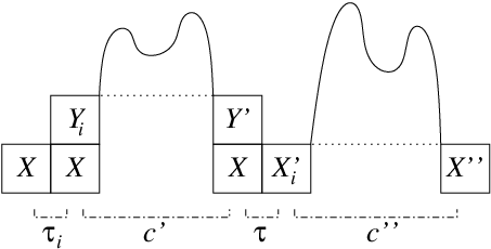
We can now use the induction hypothesis twice, resulting in:

and

If we combine this with the definition of $p_{{\cal A}}$, we obtain:

Since ${\cal A}$ has the SPP, $X_{i}^{\prime}$ is unique to $\tau_{i}$ and the output strings in $L_{\tau_{i}}$ are precisely those that can be obtained by concatenating an output string in $L_{Y_{i}}$ and an output string in $L_{X_{i}^{\prime}}$. Therefore $\Sigma_{v^{\prime}\in L_{\tau_{i}}}\ p_{{\cal G}}(\overline{v^{\prime}})$ $=$ $\Sigma_{v^{\prime}_{1}\in L_{Y_{i}}}\Sigma_{v^{\prime}_{2}\in L_{X_{i}^{\prime}}}\ p_{{\cal G}}(\overline{v^{\prime}_{1}}\overline{v^{\prime}_{2}})$ $=$ $\Sigma_{v^{\prime}_{1}\in L_{Y_{i}}}\ p_{{\cal G}}(\overline{v^{\prime}_{1}})$ $\cdot$ $\Sigma_{v^{\prime}_{2}\in L_{X_{i}^{\prime}}}\ p_{{\cal G}}(\overline{v^{\prime}_{2}})$, and

This concludes the proof.   

Note that the definition of $p_{{\cal A}}$ in the above proof relies on the strings output by ${\cal A}$. This is the main reason why we needed to consider push-down transducers rather than push-down automata (defined below). Now assume an appropriate probability function $p_{{\cal A}}$ has been found such that $({\cal A},p_{{\cal A}})$ is a PPDT that assigns the same probabilities to computations as the given PCFG assigns to the corresponding derivations, following the construction from the proof above. Then the probabilities assigned to strings over the input alphabet are also equal. We may subsequently ignore the output strings if the application at hand merely requires probabilistic recognition rather than probabilistic transduction, or in other words, we may simplify push-down transducers to push-down automata.

Formally, a push-down automaton (PDA) ${\cal A}$ is a 5-tuple $(\Sigma,$ $Q,$ $X_{\it init},$ $X_{\it final},$ $\Delta)$, where $\Sigma$ is the input alphabet, and $Q,$ $X_{\it init},$ $X_{\it final}$ and $\Delta$ are as in the definition of PDTs. Push and pop transitions are as before, but swap transitions are simplified to the form ${X}\stackrel{{\scriptstyle x}}{{\mapsto}}{Y}$, where $x\in\{\epsilon\}\cup\Sigma$. Computations are defined as in the case of PDTs, except that configurations are now pairs $(\alpha,w)$ whereas they were triples $(\alpha,w,v)$ in the case of PDTs. A probabilistic push-down automaton (PPDA) is a pair $({\cal A},p_{{\cal A}})$, where ${\cal A}$ is a PDA and $p_{{\cal A}}$ is a probability function subject to the same constraints as in the case of PPDTs. Since the definitions of CPP and SPP for PDTs did not refer to output strings, these notions carry over to PDAs in a straightforward way.

We define the size of a CFG as $\sum_{(A\rightarrow\alpha)\in R}|A\alpha|$, the total number of occurrences of terminals and nonterminals in the set of rules. Similarly, we define the size of a PDA as $\sum_{({\alpha}\mapsto{\beta})\in\Delta}|\alpha\beta|+\sum_{({X}\stackrel{{\scriptstyle x}}{{\mapsto}}{Y})\in\Delta}|{\it XxY}|$, the total number of occurrences of stack symbols and terminals in the set of transitions.

Let ${\cal A}$ $=$ $(\Sigma,$ $Q,$ $X_{\it init},$ $X_{\it final},$ $\Delta)$ be a PDA with both CPP and SPP. We will now show that we can construct an equivalent CFG ${\cal G}$ = $(\Sigma,$ $Q,$ $X_{\it init},$ $R)$ with size linear in the size of ${\cal A}$. The rules of this grammar are the following.

• •

  $X\rightarrow\it YZ$ for each transition ${X}\mapsto{XY}$, where $Z$ is the unique stack symbol such that there is at least one transition ${XY^{\prime}}\mapsto{Z}$ with $Y\leadsto Y^{\prime}$;

• •

  $X\rightarrow xY$ for each transition ${X}\stackrel{{\scriptstyle x}}{{\mapsto}}{Y}$;

• •

  $Y\rightarrow\epsilon$ for each stack symbol $Y$ such that there is at least one transition ${XY}\mapsto{Z}$ or such that $Y=X_{\it final}$.

It is easy to see that there exists a bijection from complete computations of ${\cal A}$ to complete derivations of ${\cal G}$, preserving the recognized/derived strings. Apart from an additional derivation step by rule $X_{\it final}\rightarrow\epsilon$, the complete derivations also have the same length as the corresponding complete computations.

The above construction can straightforwardly be extended to probabilistic PDAs (PPDAs). Let $({\cal A},p_{{\cal A}})$ be a PPDA with both CPP and SPP. Then we construct ${\cal G}$ as above, and further define $p_{{\cal G}}$ such that $p_{{\cal G}}(\pi)=p_{{\cal A}}(\tau)$ for rules $\pi=X\rightarrow\it YZ$ or $\pi=X\rightarrow xY$ that we construct out of transitions $\tau={X}\mapsto{XY}$ or $\tau={X}\stackrel{{\scriptstyle x}}{{\mapsto}}{Y}$, respectively, in the first two items above. We also define $p_{{\cal G}}(Y\rightarrow\epsilon)=1$ for rules $Y\rightarrow\epsilon$ obtained in the third item above. If $({\cal A},p_{{\cal A}})$ is reduced, proper and consistent then so is $({\cal G},p_{{\cal G}})$.

This leads to the observation that parsing strategies with the CPP and the SPP as well as their probabilistic extensions can also be described as grammar transformations, as follows. A given (P)CFG is mapped to an equivalent (P)PDT by a (probabilistic) parsing strategy. By ignoring the output components of swap transitions we obtain a (P)PDA, which can be mapped to an equivalent (P)CFG as shown above. This observation gives rise to an extension with probabilities of the work on covers by [31, 23].

It has been shown by [15] that there is an infinite family of languages with the following property. The sizes of the smallest CFGs generating those languages are at least quadratically larger than the sizes of the smallest equivalent PDAs. Note that this increase in size cannot occur if PDAs satisfy both the CPP and the SPP, as we have shown above.

It is always possible to transform a PDA with the CPP but without the SPP to an equivalent PDA with both CPP and SPP, by a construction that increases the size of the PDA considerably (at least quadratically, in the light of the above construction and [15]). However, such transformations in general do not preserve parsing strategies and therefore are of minor interest to the issues discussed in this paper.

The simple relationship between PDAs with both CPP and SPP on the one hand and CFGs on the other can be used to carry over algorithms originally designed for CFGs to PDAs or PDTs. One such application is the evaluation of the right-hand side of equation (1) in the proof of Theorem 4. Both the numerator and the denominator involve potentially infinite sets of subcomputations, and therefore it is not immediately clear that the proof is constructive. However, there are published algorithms to compute, for a given PCFG $({\cal G}^{\prime},p_{{\cal G}^{\prime}})$ that is not necessarily proper and a given nonterminal $A$, the expression $\Sigma_{w\in\Sigma^{\ast}}\ p_{{\cal G}^{\prime}}(A\Rightarrow^{\ast}w)$, or rather, to approximate it with arbitrary precision; see [4, 44]. This can be used to compute e.g. $\Sigma_{v\in L_{X}}\ p_{{\cal G}}(\overline{v})$ in equation (1), as follows.

The first step is to map the PDT to a CFG ${\cal G}^{\prime}$ as shown above. We then define a function $p_{{\cal G}^{\prime}}$ that assigns probability 1 to all rules that we construct out of push and pop transitions. We also let $p_{{\cal G}^{\prime}}$ assign probability $p_{{\cal G}}(\overline{y})$ to a rule $X\rightarrow xY$ that we construct out of a scan transition ${X}\stackrel{{\scriptstyle x,y}}{{\mapsto}}{Y}$. It is easy to see that, for any stack symbol $X$, we have $\Sigma_{v\in L_{X}}\ p_{{\cal G}}(\overline{v})=\Sigma_{w\in\Sigma_{1}^{\ast}}\ p_{{\cal G}^{\prime}}(X\Rightarrow^{\ast}w)$. This allows our problem on the computations of probabilities in the right-hand side of equation (1) to be reduced to a problem on PCFGs, which can be solved by existing algorithms as discussed above.

Many well-known parsing strategies with the CPP also have the SPP, such as top-down parsing [17], left-corner parsing [34] and PLR parsing [42], the first two of which we will define explicitly here, whereas of the third we will merely present a sketch. A fourth strategy that we will discuss is a combination of left-corner and top-down parsing, with special computational properties.

In order to simplify the presentation, we allow a new type of transition, without increasing the power of PDTs, viz. a combined push/swap transition of the form ${X}\stackrel{{\scriptstyle x,y}}{{\mapsto}}{XY}$. Such a transition can be seen as short-hand for two transitions, the first of the form ${X}\mapsto{XY_{x,y}}$, where $Y_{x,y}$ is a new symbol not already in $Q$, and the second of the form ${Y_{x,y}}\stackrel{{\scriptstyle x,y}}{{\mapsto}}{Y}$.

The first strategy we discuss is top-down parsing. For a fixed CFG grammar ${\cal G}=(\Sigma,$ $N,$ $S,$ $R)$, we define ${\cal S}_{\it TD}({\cal G})=({\cal A},f)$. Here ${\cal A}$ $=$ $(\Sigma,$ $R,$ $Q,$ $[S\rightarrow\ \mathrel{\bullet}\sigma],$ $[S\rightarrow\sigma\mathrel{\bullet}],$ $\Delta)$, where $Q=\{[A\rightarrow\alpha\mathrel{\bullet}\beta]\ |\ (A\rightarrow\alpha\beta)\in R\}$; these ‘dotted rules’ are well-known from [21, 14]. The transitions in $\Delta$ are:

• •

  ${[A\rightarrow\alpha\mathrel{\bullet}a\beta]}\stackrel{{\scriptstyle a,\epsilon}}{{\mapsto}}{[A\rightarrow\alpha a\mathrel{\bullet}\beta]}$ for each rule $A\rightarrow\alpha a\beta$;

• •

  ${[A\rightarrow\alpha\mathrel{\bullet}B\beta]}\stackrel{{\scriptstyle\epsilon,\pi}}{{\mapsto}}{[A\rightarrow\alpha\mathrel{\bullet}B\beta]\ [B\rightarrow\ \mathrel{\bullet}\gamma]}$ for each pair of rules $A\rightarrow\alpha B\beta$ and $\pi=B\rightarrow\gamma$;

• •

  ${[A\rightarrow\alpha\mathrel{\bullet}B\beta]\ [B\rightarrow\gamma\mathrel{\bullet}]}\mapsto{[A\rightarrow\alpha B\mathrel{\bullet}\beta]}$.

The function $f$ is the identity function on strings over $R$. If seen as a function on computations, then $f$ is a bijection from complete computations of ${\cal A}$ to complete derivations of ${\cal G}$, as required by the definition of ‘parsing strategy’.

If ${\cal G}$ is reduced, then ${\cal A}$ clearly has the CPP. That it also has the SPP can be argued as follows. Let us first remark that if $[A\rightarrow\alpha\mathrel{\bullet}\beta]\leadsto X$ for some stack symbols $[A\rightarrow\alpha\mathrel{\bullet}\beta]$ and $X$, then $X$ must be of the form $[A\rightarrow\alpha\gamma\mathrel{\bullet}\delta]$, for some $\gamma$ and $\delta$ such that $\gamma\delta=\beta$. Now, if there are three transitions ${X}\mapsto{XY}$, ${XY_{1}}\mapsto{Z_{1}}$ and ${XY_{2}}\mapsto{Z_{2}}$ such that $Y\leadsto Y_{1}$ and $Y\leadsto Y_{2}$, then $X$ must be of the form $[A\rightarrow\alpha\mathrel{\bullet}B\beta]$ and $Y$ of the form $[B\rightarrow\ \mathrel{\bullet}\gamma]$ (strictly speaking $[B\rightarrow\ \mathrel{\bullet}\gamma]_{\epsilon,\pi}$), $Y_{1}$ and $Y_{2}$ must both be $[B\rightarrow\gamma\mathrel{\bullet}]$, and $Z_{1}$ and $Z_{2}$ must both be $[A\rightarrow\alpha B\mathrel{\bullet}\beta]$. Hence the SPP is satisfied.

References

- [1] S. Abney, D. McAllester, and F. Pereira. Relating probabilistic grammars and automata. In 37th Annual Meeting of the Association for Computational Linguistics, Proceedings of the Conference, pages 542–549, Maryland, USA, June 1999.
- [2] S. Billot and B. Lang. The structure of shared forests in ambiguous parsing. In 27th Annual Meeting of the Association for Computational Linguistics, Proceedings of the Conference, pages 143–151, Vancouver, British Columbia, Canada, June 1989.
- [3] N. Blum and R. Koch. Greibach normal form transformation revisited. Information and Computation, 150:112–118, 1999.
- [4] T.L. Booth and R.A. Thompson. Applying probabilistic measures to abstract languages. IEEE Transactions on Computers, C-22(5):442–450, May 1973.
- [5] T. Briscoe and J. Carroll. Generalized probabilistic LR parsing of natural language (corpora) with unification-based grammars. Computational Linguistics, 19(1):25–59, 1993.
- [6] E. Charniak. Statistical Language Learning. MIT Press, 1993.
- [7] E. Charniak. Immediate-head parsing for language models. In 39th Annual Meeting and 10th Conference of the European Chapter of the Association for Computational Linguistics, Proceedings of the Conference, pages 116–123, Toulouse, France, July 2001.
- [8] E. Charniak and G. Carroll. Context-sensitive statistics for improved grammatical language models. In Proceedings Twelfth National Conference on Artificial Intelligence, volume 1, pages 728–733, Seattle, Washington, 1994.
- [9] C. Chelba and F. Jelinek. Exploiting syntactic structure for language modeling. In 36th Annual Meeting of the Association for Computational Linguistics and 17th International Conference on Computational Linguistics, volume 1, pages 225–231, Montreal, Quebec, Canada, August 1998.
- [10] Z. Chi. Statistical properties of probabilistic context-free grammars. Computational Linguistics, 25(1):131–160, 1999.
- [11] Z. Chi and S. Geman. Estimation of probabilistic context-free grammars. Computational Linguistics, 24(2):299–305, 1998.
- [12] M.V. Chitrao and R. Grishman. Statistical parsing of messages. In Speech and Natural Language, Proceedings, pages 263–266, Hidden Valley, Pennsylvania, June 1990.
- [13] M. Collins. Three generative, lexicalised models for statistical parsing. In 35th Annual Meeting of the Association for Computational Linguistics, Proceedings of the Conference, pages 16–23, Madrid, Spain, July 1997.
- [14] J. Earley. An efficient context-free parsing algorithm. Communications of the ACM, 13(2):94–102, February 1970.
- [15] J. Goldstine, K. Price, and D. Wotschke. A pushdown automaton or a context-free grammar — which is more economical? Theoretical Computer Science, 18:33–40, 1982.
- [16] J. Goodman. Semiring parsing. Computational Linguistics, 25(4):573–605, 1999.
- [17] M.A. Harrison. Introduction to Formal Language Theory. Addison-Wesley, 1978.
- [18] K. Inui et al. Probabilistic GLR parsing. In H. Bunt and A. Nijholt, editors, Advances in Probabilistic and other Parsing Technologies, chapter 5, pages 85–104. Kluwer Academic Publishers, 2000.
- [19] F. Jelinek and J.D. Lafferty. Computation of the probability of initial substring generation by stochastic context-free grammars. Computational Linguistics, 17(3):315–323, 1991.
- [20] D. Jurafsky and J.H. Martin. Speech and Language Processing. Prentice-Hall, 2000.
- [21] D.E. Knuth. On the translation of languages from left to right. Information and Control, 8:607–639, 1965.
- [22] B. Lang. Deterministic techniques for efficient non-deterministic parsers. In Automata, Languages and Programming, 2nd Colloquium, Lecture Notes in Computer Science, volume 14, pages 255–269, Saarbrücken, 1974. Springer-Verlag.
- [23] R. Leermakers. How to cover a grammar. In 27th Annual Meeting of the Association for Computational Linguistics, Proceedings of the Conference, pages 135–142, Vancouver, British Columbia, Canada, June 1989.
- [24] H. Leung and D. Wotschke. On the size of parsers and LR()-grammars. Theoretical Computer Science, 242:59–69, 2000.
- [25] C.D. Manning and H. Schütze. Foundations of Statistical Natural Language Processing. Massachusetts Institute of Technology, 1999.
- [26] M.-J. Nederhof. Generalized left-corner parsing. In Sixth Conference of the European Chapter of the Association for Computational Linguistics, Proceedings of the Conference, pages 305–314, Utrecht, The Netherlands, April 1993.
- [27] M.-J. Nederhof. An optimal tabular parsing algorithm. In 32nd Annual Meeting of the Association for Computational Linguistics, Proceedings of the Conference, pages 117–124, Las Cruces, New Mexico, USA, June 1994.
- [28] M.-J. Nederhof and J.J. Sarbo. Increasing the applicability of LR parsing. In H. Bunt and M. Tomita, editors, Recent Advances in Parsing Technology, chapter 3, pages 35–57. Kluwer Academic Publishers, 1996.
- [29] M.-J. Nederhof and G. Satta. Probabilistic parsing strategies. In J. Dassow, M. Hoeberechts, H. Jürgensen, and D. Wotschke, editors, Descriptional Complexity of Formal Systems (DCFS), Pre-Proceedings of a Workshop, Report No. 586, Department of Computer Science, University of Western Ontario, pages 216–230, London, Canada, August 2002.
- [30] S.-K. Ng and M. Tomita. Probabilistic LR parsing for general context-free grammars. In Proc. of the Second International Workshop on Parsing Technologies, pages 154–163, Cancun, Mexico, February 1991.
- [31] A. Nijholt. Context-Free Grammars: Covers, Normal Forms, and Parsing, Lecture Notes in Computer Science, volume 93. Springer-Verlag, 1980.
- [32] P.W. Purdom, Jr. and C.A. Brown. Parsing extended LR() grammars. Acta Informatica, 15:115–127, 1981.
- [33] B. Roark and M. Johnson. Efficient probabilistic top-down and left-corner parsing. In 37th Annual Meeting of the Association for Computational Linguistics, Proceedings of the Conference, pages 421–428, Maryland, USA, June 1999.
- [34] D.J. Rosenkrantz and P.M. Lewis II. Deterministic left corner parsing. In IEEE Conference Record of the 11th Annual Symposium on Switching and Automata Theory, pages 139–152, 1970.
- [35] J.-A. Sánchez and J.-M. Benedí. Consistency of stochastic context-free grammars from probabilistic estimation based on growth transformations. IEEE Transactions on Pattern Analysis and Machine Intelligence, 19(9):1052–1055, September 1997.
- [36] E.S. Santos. Probabilistic grammars and automata. Information and Control, 21:27–47, 1972.
- [37] E.S. Santos. Probabilistic pushdown automata. Journal of Cybernetics, 6:173–187, 1976.
- [38] S.M. Shieber, Y. Schabes, and F.C.N. Pereira. Principles and implementation of deductive parsing. Journal of Logic Programming, 24:3–36, 1995.
- [39] K. Sikkel. Parsing Schemata. Springer-Verlag, 1997.
- [40] K. Sikkel and A. Nijholt. Parsing of context-free languages. In G. Rozenberg and A. Salomaa, editors, Handbook of Formal Languages. Vol 2: Linear Modeling: Background and Applications, chapter 2, pages 61–100. Springer-Verlag, 1997.
- [41] S. Sippu and E. Soisalon-Soininen. Parsing Theory, Vol. II: LR() and LL() Parsing, EATCS Monographs on Theoretical Computer Science, volume 20. Springer-Verlag, 1990.
- [42] E. Soisalon-Soininen and E. Ukkonen. A method for transforming grammars into LL() form. Acta Informatica, 12:339–369, 1979.
- [43] V. Sornlertlamvanich et al. Empirical support for new probabilistic generalized LR parsing. Journal of Natural Language Processing, 6(3):3–22, 1999.
- [44] A. Stolcke. An efficient probabilistic context-free parsing algorithm that computes prefix probabilities. Computational Linguistics, 21(2):167–201, 1995.
- [45] F. Tendeau. Stochastic parse-tree recognition by a pushdown automaton. In Fourth International Workshop on Parsing Technologies, pages 234–249, Prague and Karlovy Vary, Czech Republic, September 1995.
- [46] F. Tendeau. Analyse syntaxique et sémantique avec évaluation d’attributs dans un demi-anneau. PhD thesis, University of Orléans, 1997.
- [47] E. Villemonte de la Clergerie. Automates à Piles et Programmation Dynamique — DyALog: Une application à la Programmation en Logique. PhD thesis, Université Paris VII, 1993.
- [48] F. Voisin. A bottom-up adaptation of Earley’s parsing algorithm. In Programming Languages Implementation and Logic Programming, International Workshop, Lecture Notes in Computer Science, volume 348, pages 146–160, Orléans, France, May 1988. Springer-Verlag.
- [49] J. Wright, A. Wrigley, and R. Sharman. Adaptive probabilistic generalized LR parsing. In Proc. of the Second International Workshop on Parsing Technologies, pages 100–109, Cancun, Mexico, February 1991.
- [50] J.H. Wright and E.N. Wrigley. GLR parsing with probability. In M. Tomita, editor, Generalized LR Parsing, chapter 8, pages 113–128. Kluwer Academic Publishers, 1991.