Preemptive Scheduling of Equal-Length Jobs
to Maximize Weighted Throughput

Philippe Baptiste Thanks: CNRS LIX, Ecole Polytechnique, 91128 Palaiseau, France. baptiste@lix.polytechnique.fr. Marek Chrobak Thanks: Department of Computer Science, University of California, Riverside, CA 92521. Supported by NSF grants CCR-9988360 and CCR-0208856. {marek,wojtek}@cs.ucr.edu. Christoph Dürr Thanks: Laboratoire de Recherche en Informatique, Université Paris-Sud, 91405 Orsay, France. durr@lri.fr. Supported by the EU 5th framework programs QAIP IST-1999-11234 and RAND-APX IST-1999-14036, and by CNRS/STIC 01N80/0502 and 01N80/0607 grants. Wojciech Jawor²²footnotemark: 2 Nodari Vakhania Thanks: Facultad de Ciencias, Universidad Autonoma del Estado de Morelos, 62251 Cuernavaca, Morelos, Mexico. nodari@servm.fc.uaem.mx. Supported by CONACyT-NSF cooperative research grant E120.19.14.

Abstract

We study the problem of computing a preemptive schedule of equal-length jobs with given release times, deadlines and weights. Our goal is to maximize the weighted throughput, which is the total weight of completed jobs. In Graham’s notation this problem is described as $(1|r_{j};p_{j}{=}p;\text{pmtn}|\sum w_{j}U_{j})$ . We provide an $O(n^{4})$ -time algorithm for this problem, improving the previous bound of $O(n^{10})$ by Baptiste [Bap99b].

1 Introduction

We study the following scheduling problem. We are given a set of $n$ jobs of the same integer length $p\geq 1$ . For each job $j$ we are also given three integer values: its release time $r_{j}$ , deadline $d_{j}$ and weight $w_{j}\geq 0$ . Our goal is to compute a preemptive schedule that maximizes the weighted throughput, which is the total weight of completed jobs. Alternatively, this is sometimes formulated as minimizing the weighted number of late jobs. In Graham’s notation, this scheduling problem is described as $(1|r_{j};p_{j}{=}p;\text{pmtn}|\sum w_{j}U_{j})$ , where $U_{j}$ is a 0-1 variable indicating whether $j$ is completed or not in the schedule.

Most of the literature on job scheduling focuses on minimizing makespan, lateness, tardiness, or other objective functions that depend on the completion time of all jobs. Our work is motivated by applications in real-time overloaded systems, where the total workload often exceeds the capacity of the processor, and where the job deadlines are critical, in the sense that the jobs that are not completed by the deadline bring no benefit and may as well be removed from the schedule altogether. In such systems, a reasonable goal is to maximize the throughput, that is, the number of executed tasks. In more general situations, some jobs may be more important than other. This can be modeled by assigning weights to the jobs and maximizing the weighted throughput (see, for example, [KS95]).

The above problem $(1|r_{j};p_{j}{=}p;\text{pmtn}|\sum w_{j}U_{j})$ was studied by Baptiste [Bap99b], who showed that it can be solved in polynomial time. His algorithm runs in time $O(n^{10})$ . In this paper we improve his result by providing an $O(n^{4})$ -time algorithm for this problem.

$1\|p_{i}{=}p;r_{j};\text{pmtn}\|\sum U_{j}$ $O(n\log n)$ [Law94]	$1\|r_{j};\text{pmtn}\|\sum U_{j}$ $O(n^{5})$ [Law90] $O(n^{4})$ [Bap99a] $2\|r_{j};\text{pmtn}\|\sum U_{j}$ NP-hard [DLW92]		$1\|p_{i}{=}p;r_{j}\|\sum U_{j}$ $O(n^{3}\log n)$ [Car81]
$1\|p_{i}{=}p;r_{j};\text{pmtn}\|\sum w_{j}U_{j}$ $O(n^{4})$ [this paper] was $O(n^{10})$ [Bap99b] if $r_{i}<r_{j}\Rightarrow w_{i}\geq w_{j}$ $O(n\log n)$ [Law94]	$1\|r_{j};\text{pmtn}\|\sum w_{j}U_{j}$ NP-hard [GJ79] pseudo-polynomial [Law90]	$P\|p_{i}{=}p;\text{pmtn}\|\sum w_{j}U_{j}$ NP-hard [BK99] $Pm\|p_{i}{=}p;\text{pmtn}\|\sum w_{j}U_{j}$ $O(n^{2^{m}m!})$ [Bap00] $O(nm(\max d_{j})^{m})$ [Bap00]	$1\|p_{i}{=}p;r_{j}\|\sum w_{j}U_{j}$ $O(n^{7})$ [Bap99b] $Pm\|p_{i}\,=\,p;r_{j}\|\sum w_{j}U_{j}$ $O(n^{6m+1})$ [BBKT02]

Figure 1: Complexity of some related throughput maximization problems.

Figure 1 shows some complexity results for related scheduling problems where the objective function is to maximize throughput. A more extensive overview can be found at Brucker and Knust’s website [BK]. (That website, however, only categorizes problems as NP-complete, polynomial, pseudo-polynomial or open, without describing their exact time complexity.)

2 Preliminaries

Terminology and notation.

We assume that the jobs on input are numbered $1,2,\dots,n$ . All jobs have the same integer length $p\geq 1$ . Each job $j$ is specified by a triple $(r_{j},d_{j},w_{j})$ of integers, where $r_{j}$ is the release time, $d_{j}$ is the deadline, and $w_{j}\geq 0$ is the weight of $j$ . Without loss of generality, we assume that $d_{j}\geq r_{j}+p$ for all $j$ and that $\min_{j}r_{j}=0$ .

Throughout the paper, by a time unit $t$ we mean a time interval $[t,t+1)$ , where $t$ is an integer. A preemptive schedule (or, simply, a schedule) $S$ is a function that assigns to each job $j$ a set $S(j)$ of time units when $j$ is executed. Here, the term “preemption” refers to the fact that the time units in $S$ may not be consecutive. We require that $S$ satisfies the following two conditions:

: (sch1) $S(j)\subseteq[r_{j},d_{j})$ for each $j$ (jobs are executed between their release times and deadlines.)
: (sch2) $S(i)\cap S(j)=\emptyset$ for $i\neq j$ (at most one job is executed at a time.)

If $t\in S(j)$ then we say that (a unit of) $j$ is scheduled or executed at time unit $t$ . If $|S(j)|=p$ , then we say that $S$ completes $j$ . The completion time of $j$ is $C_{j}=1+\max S(j)$ . Without loss of generality, we will be assuming that each job $j$ is either completed ( $|S(j)|=p$ ) or not executed at all ( $S(j)=\emptyset$ ).

The throughput of $S$ is the total weight of jobs that are completed in $S$ , that is $w(S)=\sum_{|S(j)|=p}w_{j}$ . Our goal is to find a schedule of all jobs with maximum throughput.

For a set of jobs ${\cal J}$ , by $w({\cal J})=\sum_{j\in{\cal J}}w_{j}$ we denote the total weight of ${\cal J}$ . Given a set of jobs ${\cal J}$ , if there is a schedule $S$ that completes all jobs in ${\cal J}$ , then we say that ${\cal J}$ is feasible. The restriction of $S$ to ${\cal J}$ is called a full schedule of ${\cal J}$ .

Earliest-deadline schedules.

For two jobs $j,k$ , we say that $j$ is more urgent than $k$ if $d_{j}<d_{k}$ . It is well-known that if ${\cal J}$ is feasible, then ${\cal J}$ can be fully scheduled using the following earliest-deadline rule: at every time step $t$ , execute the most urgent job among the jobs that have been released by time $t$ but not yet completed. Ties can can be broken arbitrarily, but consistently, for example, always in favor of lower numbered jobs. If $S$ is any schedule (of all jobs), then we say that $S$ is earliest-deadline if its restriction to the set of executed jobs is earliest-deadline.

Since any feasible set of jobs ${\cal J}$ can be fully scheduled in time $O(n\log n)$ using the earliest-deadline rule, the problem of computing a schedule of maximum throughput is essentially equivalent to computing a maximum-weight feasible set.

Refer to caption — Figure 2: Examples of earliest-deadline schedules with $p=3$ . The rectangles represent intervals $[r_{j},d_{j})$ , and the shaded areas show time units where jobs are executed. The first schedule consists of two distinct blocks. After removing the least urgent job $5$ , the second block splits into several smaller blocks.

Each earliest-deadline schedule $S$ has the following structure. The time axis is divided into busy intervals (when jobs are being executed) called blocks and idle intervals called gaps. Each block is an interval $[r_{i},C_{j})$ between a release time $r_{i}$ and a completion time $C_{j}$ , and it satisfies the following two properties: (b1) all jobs executed in this block are not released before $r_{i}$ , and (b2) $C_{j}$ is the first completion time after $r_{i}$ such that all jobs in $S$ released before $C_{j}$ are completed at or before $C_{j}$ . Note that $C_{j}-r_{i}=ap$ , for $a$ equal to the number of jobs executed in this block. Figure 2 shows two examples of earliest-deadline schedules.

In some degenerate situations, where the differences between release times are multiples of $p$ , a gap can be empty, and the end $C_{j}$ of one block then equals the beginning $r_{m}$ of the next block.

The above structure is recursive, in the following sense. Let $k$ be the least urgent job scheduled in a given block $[r_{i},C_{j})$ . Then the last completed job is $k$ . Also, when we remove job $k$ from the schedule, without any further modifications, we obtain again an earliest-deadline-schedule for the set of remaining jobs (See Figure 2). The interval $[r_{i},C_{j})$ may now contain several blocks of this new schedule.

2.1 An $O(n^{4})$ -Time Algorithm

We assume that the jobs are ordered $1,2,\dots,n$ according to non-decreasing deadlines, that is $d_{1}\leq d_{2}\leq\ldots\leq d_{n}$ . Without loss of generality we may assume that job $n$ is a “dummy” job with $w_{n}=0$ and $r_{n}=d_{n-1}$ (otherwise, we can add one such additional job). We use letters $i,j,k,l\in[1,n]$ for job identifiers, and $a,b\in[0,n]$ for numbers of jobs.

Given an interval $[x,y)$ , define a set ${\cal J}$ of jobs to be $(k,x,y)$ -feasible if

: (f1) ${\cal J}\subseteq{\left\{1,2,\dots,k\right\}}$ ,
: (f2) $r_{j}\in[x,y)$ for all $j\in{\cal J}$ , and
: (f3) ${\cal J}$ has a full schedule in $[x,y)$ (that is, all jobs are completed by time $y$ .)

An earliest-deadline schedule of a $(k,x,y)$ -feasible set of jobs will be called a $(k,x,y)$ -schedule. If ties are broken consistently, then there is a 1-1 correspondence between feasible sets of jobs and their earliest-deadline schedules. Thus, for the sake of simplicity, we will use the same notation ${\cal J}$ for a feasible set of jobs and for its earliest-deadline schedule.

Note that if $e$ is the job with the earliest release time, then an optimal $(n,r_{e},r_{n})$ -schedule is also an optimal schedule to the whole instance. The idea of the algorithm is to compute optimal $(k,r_{i},r_{j})$ -schedules ${\cal F}^{k}_{i,j}$ in bottom-up order, using dynamic programming. As there does not seem to be an efficient way to express ${\cal F}^{k}_{i,j}$ in terms of such sets for smaller instances, we use two auxiliary optimal schedules denoted ${\cal G}^{k}_{i,a}$ and ${\cal H}^{k}_{i,j}$ on which we impose some additional restrictions.

We first define the values $F^{k}_{i,j}$ , $G^{k}_{i,j}$ , and $H^{k}_{i,a}$ that are meant to represent the weights of the corresponding schedules mentioned above. The interpretation of these values is as follows:

$F^{k}_{i,j}$	=	the optimal weight of a $(k,r_{i},r_{j})$ -schedule.
$G^{k}_{i,a}$	=	the optimal weight of a $(k,r_{i},r_{i}+ap)$ -schedule that consists of a single block starting at time $r_{i}$ and ending at $r_{i}+ap$ .
$H^{k}_{i,j}$	=	the optimal weight of a $(k,r_{i},r_{j})$ -schedule that has no gap between $r_{i}$ and $r_{k+1}$ .

In $F^{k}_{i,j}$ and $H^{k}_{i,j}$ we assume that $r_{i}\leq r_{j}$ . In $H^{k}_{i,j}$ we additionally assume that $k<n$ and $r_{i}\leq r_{k+1}$ .

We now give recursive formulas these values. In these formulas we use the following auxiliary functions:

$\displaystyle{\Delta}(x,y)$	$\displaystyle=$	$\displaystyle\min{\left\{n,{\left\lceil\frac{y-x}{p}\right\rceil}-1\right\}}$
$\displaystyle{\lambda}(x)$	$\displaystyle=$	$\displaystyle{\mbox{\rm argmin}}_{i}{\left\{r_{i}:r_{i}\geq x\right\}}$
$\displaystyle{\lambda^{+}}(x)$	$\displaystyle=$	$\displaystyle{\mbox{\rm argmin}}_{i}{\left\{r_{i}:r_{i}>x\right\}}$

Thus ${\Delta}(x,y)$ is the maximum number of jobs (but not more than $n$ ) that can be executed between $x$ and $y$ (ignoring release times and deadlines), such that the interval $[x,y)$ is not completely filled. For $x\leq r_{n}$ , ${\lambda}(x)$ denotes the first job released at or after $x$ . Similarly, for $x<r_{n}$ , ${\lambda^{+}}(x)$ is the first job released strictly after $x$ . (Ties can be broken arbitrarily).

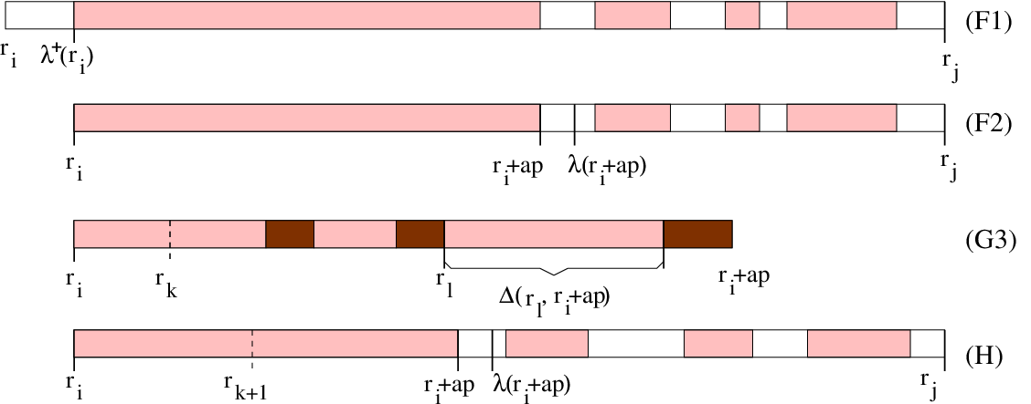
Values $F^{k}_{i,j}$ . If $r_{j}=r_{i}$ then $F^{k}_{i,j}=0$ . Otherwise, $F^{k}_{i,j}$ is defined inductively as follows:

\displaystyle F^{k}_{i,j}

\displaystyle=

\displaystyle\max\left\{\begin{array}[]{lclr}\displaystyle F^{k}_{{\lambda^{+}}(r_{i}),j}&&&(F1)\\ \\ \displaystyle\max_{\begin{subarray}{c}1\leq a\leq n\\ r_{i}+ap\leq r_{j}\end{subarray}}{\left\{G^{k}_{i,a}+F^{k}_{{\lambda}(r_{i}+ap),j}\right\}}&&&(F2)\end{array}\right.

Note that in (F1) ${\lambda^{+}}(r_{i})$ is well defined since $r_{i}<r_{j}$ , and in (F2) ${\lambda}(r_{i}+ap)$ is well defined since $r_{i}+ap\leq r_{j}$ .

Values $G^{k}_{i,a}$ . If $k=0$ or $a=0$ , then $G^{k}_{i,a}=0$ . If $r_{k}\not\in[r_{i},r_{i}+(a-1)p]$ or $d_{k}<r_{i}+ap$ then $G^{k}_{i,a}=G^{k-1}_{i,a}$ . Otherwise, $G^{k}_{i,a}$ is defined as follows:

\displaystyle G^{k}_{i,a}

\displaystyle=

\displaystyle\max\left\{\begin{array}[]{lclr}\displaystyle G^{k-1}_{i,a}&&&(G1)\\ \\ \displaystyle G^{k-1}_{i,a-1}+w_{k}&&&(G2)\\ \\ \displaystyle\max_{r_{k}<r_{l}<r_{i}+ap}{\left\{H^{k-1}_{i,l}+G^{k-1}_{l,{\Delta}(r_{l},r_{i}+ap)}+w_{k}\right\}}&&&(G3)\end{array}\right.

Values $H^{k}_{i,j}$ . If $r_{j}=r_{i}$ then $H^{k}_{i,j}=0$ . If $k=n$ or $r_{k+1}\not\in[r_{i},r_{j}]$ then $H^{k}_{i,j}$ is undefined. For other values $H^{k}_{i,j}$ is defined inductively as follows:

\displaystyle H^{k}_{i,j}

\displaystyle=

\displaystyle\begin{array}[]{lclr}\displaystyle\max_{\begin{subarray}{c}0\leq a\leq n\\ r_{k+1}\leq r_{i}+ap\leq r_{j}\end{subarray}}{\left\{G^{k}_{i,a}+F^{k}_{{\lambda}(r_{i}+ap),j}\right\}}&&&(H)\end{array}

Algorithm DP.

The algorithm first computes the values $F^{k}_{i,j},G^{k}_{i,a},H^{k}_{i,j}$ bottom-up. The general structure of this first stage is as follows:


for $k{\,\leftarrow\,}0$ to $n$ do
	for $i{\,\leftarrow\,}n$ downto $1$ do
		for $a{\,\leftarrow\,}0$ to $n$ do
			compute $G^{k}_{i,a}$
		for $j{\,\leftarrow\,}i$ to $n$ do
			compute $F^{k}_{i,j}$ and $H^{k}_{i,j}$

The values $F^{k}_{i,j}$ , $G^{k}_{i,a}$ , and $H^{k}_{i,j}$ are computed according to their recursive definitions, as given earlier. At each step, we record which value realized the maximum.

In the second stage, we construct an optimal schedule ${\cal F}^{n}_{e,n}$ , where $e$ is the job with earliest deadline. This is achieved by starting with ${\cal F}^{n}_{e,n}$ and recursively reconstructing optimal schedules ${\cal F}^{k}_{i,j}$ , ${\cal G}^{k}_{i,a}$ and ${\cal H}^{k}_{i,j}$ that realize weights $F^{k}_{i,j},G^{k}_{i,a}$ , and $H^{k}_{i,j}$ , respectively, according to the following procedure.

Computing ${\cal F}^{k}_{i,j}$ . If $F^{k}_{i,j}=0$ , return ${\cal F}^{k}_{i,j}=\emptyset$ . If $F^{k}_{i,j}$ was maximized by choice (F1), let ${\cal F}^{k}_{i,j}={\cal F}^{k-1}_{{\lambda^{+}}(r_{i}),j}$ . If $F^{k}_{i,j}$ was maximized by choice (F2), let ${\cal F}^{k}_{i,j}={\cal G}^{k}_{i,a}\cup{\cal F}^{k}_{{\lambda}(r_{i}+ap),j}$ , where $a$ is the integer that realizes the maximum.

Computing $G^{k}_{i,a}$ . If $G^{k}_{i,a}=0$ , return ${\cal G}^{k}_{i,a}=\emptyset$ . If $G^{k}_{i,a}$ is realized by choice (G1), let ${\cal G}^{k}_{i,a}={\cal G}^{k-1}_{i,a}$ . If $G^{k}_{i,a}$ is realized by choice (G2), let ${\cal G}^{k}_{i,a}={\cal G}^{k-1}_{i,a-1}\cup{\left\{k\right\}}$ . If $G^{k}_{i,a}$ is realized by choice (G3), let ${\cal G}^{k}_{i,a}={\cal H}^{k-1}_{i,l}\cup{\cal G}^{k-1}_{l,{\Delta}(r_{l},r_{i}+ap)}\cup{\left\{k\right\}}$ , where $l$ is the job that realizes the maximum in (G3).

Computing ${\cal H}^{k}_{i,j}$ . If $H^{k}_{i,j}=0$ , return ${\cal H}^{k}_{i,j}=\emptyset$ . Otherwise, ${\cal H}^{k}_{i,j}={\cal G}^{k}_{i,a}\cup{\cal F}^{k}_{{\lambda}(r_{i}+ap),j}$ , where $a$ is the integer that realizes the maximum.

Theorem 2.1

Algorithm DP correctly computes a maximum-weight feasible set of jobs and it runs in time $O(n^{4})$ .

Proof: The time complexity is quite obvious: We have $O(n^{3})$ values $F^{k}_{i,j}$ , $G^{k}_{i,a}$ , $H^{k}_{i,j}$ , and they can be stored in 3-dimensional tables. The functions ${\Delta}(\cdot,\cdot)$ , ${\lambda^{+}}(\cdot)$ , and ${\lambda}(\cdot)$ can be precomputed. Then each entry in these tables can be computed in time $O(n)$ . The reconstruction of the schedules in the second part takes only time $O(n)$ .

To show correctness, we need to prove two claims:

Claim 1:

: (1f) $w({\cal F}^{k}_{i,j})=F^{k}_{i,j}$ and ${\cal F}^{k}_{i,j}$ is a $(k,r_{i},r_{j})$ -schedule.
: (1g) $w({\cal G}^{k}_{i,a})=G^{k}_{i,a}$ and ${\cal G}^{k}_{i,a}$ is $(k,r_{i},r_{i}+ap)$ -schedule that consists of a single block of $a$ jobs starting at $r_{i}$ .
: (1h) $w({\cal H}^{k}_{i,j})=H^{k}_{i,j}$ and ${\cal H}^{k}_{i,j}$ is $(k,r_{i},r_{j})$ -schedule that has no gap before $r_{k+1}$ (assuming that $k<n$ and $r_{i}\leq r_{k+1}\leq r_{j}$ .)

Claim 2:

: (2f) If ${\cal J}$ is a $(k,r_{i},r_{j})$ -schedule then $w({\cal J})\leq F^{k}_{i,j}$ .
: (2g) If ${\cal J}$ is a $(k,r_{i},r_{i}+ap)$ -schedule that is a single block of $a$ jobs then $w({\cal J})\leq G^{k}_{i,a}$ .
: (2h) If ${\cal J}$ is a $(k,r_{i},r_{j})$ -schedule that has no gap before $r_{k+1}$ then $w({\cal J})\leq H^{k}_{i,j}$ (assuming that $k<n$ and $r_{i}\leq r_{k+1}\leq r_{j}$ .)

We prove both claims by induction. We first define a partial order on all function instances $F^{k}_{i,j}$ , $G^{k}_{i,a}$ and $H^{k}_{i,j}$ . We first order them in order of increasing $k$ . For a fixed $k$ , we order them in order of increasing length of their time intervals, that is, $r_{j}-r_{i}$ for $F^{k}_{i,j}$ and $H^{k}_{i,j}$ , and $ap$ for $G^{k}_{i,a}$ . Finally, for a fixed $k$ , $i$ and $j$ , we assume that $F^{k}_{i,j}$ is before $H^{k}_{i,j}$ . The induction will proceed with respect to this ordering.

We now prove Claim 1. The base cases are when $k=0$ or $a=0$ in $G^{k}_{i,a}$ , or $r_{i}=r_{j}$ in $F^{k}_{i,j}$ and $H^{k}_{i,j}$ . In all these cases Claim 1 holds trivially. We now examine the inductive steps.

To prove (1f), if ${\cal F}^{k}_{i,j}$ was constructed from case (F1), the claim holds by induction. If ${\cal F}^{k}_{i,j}$ was constructed from case (F2), let $a$ be the integer that realizes the maximum and $l={\lambda}(r_{i}+ap)$ . Since $r_{i}+ap\leq r_{l}$ , sets ${\cal G}^{k}_{i,a}$ and ${\cal F}^{k}_{l,j}$ are disjoint, and so are the intervals $[r_{i},r_{i}+ap)$ , $[r_{l},r_{j})$ . Thus both ${\cal G}^{k}_{i,a}$ and ${\cal F}^{k}_{l,j}$ can be fully scheduled in $[r_{i},r_{j})$ and $w({\cal F}^{k}_{i,j})=w({\cal G}^{k}_{i,a})+w({\cal F}^{k}_{l,j})=G^{k}_{i,a}+F^{k}_{l,j}=F^{k}_{i,j}$ , by induction.

To prove (1g), if $G^{k}_{i,a}$ is realized by case (G1), the claim is obvious. In case (G2), we have $k\notin{\cal G}^{k-1}_{i,a-1}$ , $r_{k}\leq r_{i}+(a-1)p$ , and $d_{k}\geq r_{i}+ap$ . Thus we can schedule ${\cal G}^{k-1}_{i,a-1}$ , and then schedule $k$ at $r_{i}+(a-1)p$ . By induction, $w({\cal G}^{k}_{i,a})=w({\cal G}^{k-1}_{i,a-1})+w_{k}=G^{k-1}_{i,a-1}+w_{k}=G^{k}_{i,a}$ . In case (G3), let $l$ be the job that realizes the maximum and $b={\Delta}(r_{l},r_{i}+ap)$ . The sets ${\cal H}^{k-1}_{i,l}$ and ${\cal G}^{k-1}_{l,b}$ are disjoint and so are the intervals $[r_{i},r_{l})$ , $[r_{l},r_{l}+bp)$ . By the definition of $b$ , we have $r_{l}+bp<r_{i}+ap$ , so there is a non-zero idle time in ${\cal H}^{k-1}_{i,l}\cup{\cal G}^{k-1}_{l,b}$ between $r_{l}+bp$ and $r_{i}+ap$ . Since the total interval $[r_{i},r_{i}+ap)$ has length $ap$ , the total idle time in this interval must be at least $p$ . Moreover, all gaps occur after $r_{k}$ . This implies that we can schedule job $k$ in these idle intervals. Also, note that $w({\cal G}^{k}_{i,a})=w({\cal H}^{k-1}_{i,l})+w({\cal G}^{k-1}_{l,b})+w_{k}=H^{k-1}_{i,l}+G^{k-1}_{l,b}+w_{k}=G^{k}_{i,a}$ , so the claim holds.

To prove (1h), let $a$ be the integer that realizes the maximum in (H) and $l={\lambda}(r_{i}+ap)$ . As before, since $r_{i}+ap\leq r_{l}$ , sets ${\cal G}^{k}_{i,a}$ and ${\cal F}^{k}_{l,j}$ are disjoint, and so are the intervals $[r_{i},r_{i}+ap)$ , $[r_{l},r_{j})$ . Thus both ${\cal G}^{k}_{i,a}$ and ${\cal F}^{k}_{l,j}$ can be fully scheduled in $[r_{i},r_{j})$ and $w({\cal H}^{k}_{i,j})=w({\cal G}^{k}_{i,a})+w({\cal F}^{k}_{l,j})=G^{k}_{i,a}+F^{k}_{l,j}=H^{k}_{i,j}$ , by induction.

We now show Claim 2. Again, we proceed by induction with respect to the ordering of the instances described before the proof of Claim 1. The claim holds trivially for the base cases. We now consider the inductive step.

To prove (2f), we have two cases. If ${\cal J}$ does not start at $r_{i}$ , then it cannot start earlier than at $r_{m}$ , for $m={{\lambda^{+}}(r_{i})}$ , so the claim follows by induction. If ${\cal J}$ starts at $r_{i}$ , let $a$ be the length of its first block. The second block (if any) cannot start earlier than at $r_{l}$ , for $l={\lambda}(r_{i}+ap)$ . (Note that there might be no gap between the blocks.) We partition ${\cal J}$ into two sets: ${\cal J}_{1}$ containing the jobs scheduled in $[r_{i},r_{i}+ap)$ as a single block, and ${\cal J}_{2}$ containing the jobs scheduled in $[r_{l},r_{j})$ . By induction, $w({\cal J})=w({\cal J}_{1})+w({\cal J}_{2})\leq G^{k}_{i,a}+F^{k}_{l,j}\leq F^{k}_{i,j}$ .

We now prove (2g). If $k\notin{\cal J}$ then ${\cal J}$ is a $(k-1,r_{i},r_{i}+ap)$ -schedule, so $w({\cal J})\leq G^{k-1}_{i,a}\leq G^{k}_{i,a}$ , by induction and by case (G1). Now assume that $k\in{\cal J}$ . If job $k$ has not been interrupted, then ${\cal J}-{\left\{k\right\}}$ is a $(k-1,r_{i},r_{i}+(a-1)p)$ -schedule. Thus, by induction and (G2), $w({\cal J})\leq G^{k-1}_{i,a-1}+w_{k}\leq G^{k}_{i,a}$ .

Otherwise, let $l$ be the last job that interrupted $k$ . Starting at $r_{l}$ , ${\cal J}$ executes $b={\Delta}(r_{l},r_{i}+ap)$ jobs with deadlines smaller than $d_{k}$ , after which it executes a portion $r_{i}+ap-r_{l}-bp>0$ of job $k$ . We partition ${\cal J}-{\left\{k\right\}}$ into two sets: ${\cal J}_{1}$ containing the jobs scheduled before $r_{l}$ , and ${\cal J}_{2}$ containing the jobs scheduled after $r_{l}$ . Note that ${\cal J}_{1}\cup{\cal J}_{2}={\cal J}-{\left\{k\right\}}$ , since the jobs scheduled before $r_{l}$ must also be completed before $r_{l}$ and the other jobs cannot be released yet. By induction, sets ${\cal J}_{1}$ is a $(k-1,r_{i},r_{l})$ -schedule in which the first block starts at $r_{i}$ and ends after $r_{k}$ , and ${\cal J}_{2}$ is a single block starting at $r_{l}$ and ending at $r_{l}+bp$ . Thus, by induction and (G3), $w({\cal J})=w({\cal J}_{1})+w({\cal J}_{2})+w_{k}\leq H^{k-1}_{i,l}+G^{k-1}_{l,b}+w_{k}\leq G^{k}_{i,a}$ .

The proof of (2h) is similar. We have two subcases. Suppose first that $r_{k+1}=r_{i}$ . By induction, we have $w({\cal J})\leq F^{k}_{i,j}=H^{k}_{i,j}$ , since in this case we can choose $a=0$ in (H). If $r_{k+1}>r_{i}$ , then the first block of ${\cal J}$ starts at $r_{i}$ and ends after $r_{k+1}$ . Let $a$ be the length of its first block. The second block (if any) cannot start earlier than at $r_{l}$ , for $l={\lambda}(r_{i}+ap)$ . We partition ${\cal J}$ into two sets ${\cal J}_{1}$ containing the jobs scheduled in $[r_{i},r_{i}+ap)$ as a single block and ${\cal J}_{2}$ containing the jobs scheduled in $[r_{l},r_{j})$ . By induction, $w({\cal J})=w({\cal J}_{1})+w({\cal J}_{2})\leq G^{k}_{i,a}+F^{k}_{l,j}\leq H^{k}_{i,j}$ . $\Box$

3 Final Remarks

Several open problems remain. Although our running time $O(n^{4})$ for the scheduling problem $(1|r_{j};p_{j}{=}p;\text{pmtn}|\sum w_{j}U_{j})$ is substantially better than the previous bound of $O(n^{10})$ , it would be interesting to see whether it can be improved further. Similarly, it would be interesting to improve the running time for the non-preemptive version of this problem, $(1|r_{j};p_{j}{=}p|\sum w_{j}U_{j})$ , which is currently $O(n^{7})$ [Bap99a].

In the multi-processor case, the weighted version is known to be NP-complete [BK99], but the non-weighted version remains open. More specifically, it is not known whether the problem $(P|r_{j};p_{j}{=}p;\text{pmtn}|\sum U_{j})$ can be solved in polynomial time. (One difficulty that arises for $2$ or more processors is that we cannot restrict ourselves to earliest-deadline schedules. For example, an instance consisting of three jobs with feasible intervals $(0,3)$ , $(0,4)$ , and $(0,5)$ and processing time $p=3$ is feasible, but the earliest-deadline schedule will complete only jobs $1$ and $2$ .) In the multi-processor case, one can also consider a preemptive version where jobs are not allowed to migrate between processors.

References

[Bap99a] Philippe Baptiste. An $O(n^{4})$ algorithm for preemptive scheduling of a singler machine to minimize the number of late jobs. Operations Research Letters, 24:175–180, 1999.
[Bap99b] Philippe Baptiste. Polynomial time algorithms for minimizing the weighted number of late jobs on a single machine with equal processing times. Journal on Scheduling, 2:245–252, 1999.
[Bap00] Philippe Baptiste. Preemptive scheduling of identical machines. Technical report, Universite de Technologie de Compiegne, France., 2000.
[BBKT02] Philippe Baptiste, Peter Brucker, Sigrid Knust, and Vadim G. Timkovsky. Fourteen notes on equal-processing-time scheduling. Submitted for publication, 2002.
[BK] Peter Brucker and Sigrid Knust. Complexity results for scheduling problems. www.mathematik.uni-osnabrueck.de/research/OR/class.
[BK99] Peter Brucker and Svetlana A. Kravchenko. Preemption can make parallel machine scheduling problems hard. Osnabrücker Schriften zur Mathematik, 211, 1999.
[Car81] Jacques Carlier. Problèmes d’ordonnancement à durées égales. QUESTIO, 5(4):219–228, 1981.
[DLW92] Jianzhong Du, Joseph Y.T. Leung, and Chin S. Wong. Minimizing the number of late jobs with release time constraint. Journal on Combinatorial Mathematics and Combinatorial Computing, 11:97–107, 1992.
[GJ79] Michael R. Garey and David S. Johnson. Computers and Intractability, A Guide to the Theory of NP-completeness. Freeman, 1979.
[KS95] G. Koren and D. Shasha. $d^{over}$ : an optimal on-line scheduling algorithm for overloaded uniprocessor real-time systems. SIAM Journal on Computing, 24:318–339, 1995.
[Law90] Eugene L. Lawler. A dynamic programming algorithm for preemptive scheduling of a single machine to minimize the number of late jobs. Ann. Oper. Res., 26:125–133, 1990.
[Law94] Eugene L. Lawler. Knapsack-like scheduling problems, the Moore-Hodgson algorithm and the ‘tower of sets’ property. Mathl. Comput. Modelling, 20(2):91–106, 1994.

Preemptive Scheduling of Equal-Length Jobs to Maximize Weighted Throughput