Research supported in part by the the the Italian MIUR Projects cometa and napoli and by ASI project ARISCOM.
Soft Concurrent Constraint Programming
Abstract
Soft constraints extend classical constraints to represent multiple consistency levels, and thus provide a way to express preferences, fuzziness, and uncertainty. While there are many soft constraint solving formalisms, even distributed ones, by now there seems to be no concurrent programming framework where soft constraints can be handled. In this paper we show how the classical concurrent constraint (cc) programming framework can work with soft constraints, and we also propose an extension of cc languages which can use soft constraints to prune and direct the search for a solution. We believe that this new programming paradigm, called soft cc (scc), can be also very useful in many web-related scenarios. In fact, the language level allows web agents to express their interaction and negotiation protocols, and also to post their requests in terms of preferences, and the underlying soft constraint solver can find an agreement among the agents even if their requests are incompatible.
Keywords:
Languagescategory
D.1.3 Programming Techniques Concurrent Programmingkeywords
Distributed programmingcategory
D.3.1 Programming Languages Formal Definitions and Theorykeywords
Semantics and Syntaxcategory
D.3.2 Programming Languages Language Classificationskeywords
Concurrent, distributed, and parallel languages and Constraint and logic languagescategory
D.3.3 Programming Languages Language Constructs and Featureskeywords
Concurrent programming structures and Constraintscategory
F.3.2 Logics and Meanings of Programs Semantics of Programming Languageskeywords
Operational semanticskeywords
constraints, soft constraints, concurrent constraint programming1 Introduction
The concurrent constraint (cc) paradigm [20] is a very interesting computational framework which merges together constraint solving and concurrency. The main idea is to choose a constraint system and use constraints to model communication and synchronization among concurrent agents.
Until now, constraints in cc were crisp, in the sense that they could only be satisfied or violated. Recently, the classical idea of crisp constraints has been shown to be too weak to represent real problems and a big effort has been done toward the use of soft constraints [16, 14, 19, 15, 22, 7, 8, 3], which can have more than one level of consistency. Many real-life situations are, in fact, easily described via constraints able to state the necessary requirements of the problems. However, usually such requirements are not hard, and could be more faithfully represented as preferences, which should preferably be satisfied but not necessarily. Also, in real life, we are often challenged with over-constrained problems, which do not have any solution, and this also leads to the use of preferences or in general of soft constraints rather than classical constraints.
Generally speaking, a soft constraint is just a classical constraint plus a way to associate, either to the entire constraint or to each assignment of its variables, a certain element, which is usually interpreted as a level of preference or importance. Such levels are usually ordered, and the order reflects the idea that some levels are better than others. Moreover, one has also to say, via suitable combination operators, how to obtain the level of preference of a global solution from the preferences in the constraints.
Many formalisms have been developed to describe one or more classes of soft constraints. For instance consider fuzzy CSPs [14, 19], where crisp constraints are extended with a level of preference represented by a real number between and , or probabilistic CSPs [15], where the probability to be in the real problem is assigned to each constraint. Some other examples are partial [16] or valued CSPs [22], where a preference is assigned to each constraint, in order to satisfy as many constraints as possible, and thus handle also overconstrained problems.
We think that many network-related problem could be represented and solved by using soft constraints. Moreover, the possibility to use a concurrent language on top of a soft constraint system, could lead to the birth of new protocols with an embedded constraint satisfaction and optimization framework.
In particular, the constraints could be related to a quantity to be minimized/maximized but they could also satisfy policy requirements given for performance or administrative reasons. This leads to change the idea of QoS in routing and to speak of constraint-based routing [1, 11, 17, 9]. Constraints are in fact able to represent in a declarative fashion the needs and the requirements of agents interacting over the web.
The features of soft constraints could also be useful in representing routing problems where an imprecise state information is given [10]. Moreover, since QoS is only a specific application of a more general notion of Service Level Agreement (SLA), many applications could be enhanced by using such a framework. As an example consider E-commerce: here we are always looking for establishing an agreement between a merchant, a client and possibly a bank. Also, all auction-based transactions need an agreement protocol. Moreover, also security protocol analysis have shown to be enhanced by using security levels instead of a simple notion of secure/insecure level [2]. All these considerations advocate for the need of a soft constraint framework where optimal answers are extracted.
In this paper, we use one of the frameworks able to deal with soft constraints [6, 7]. The framework is based on a semiring structure that is equipped with the operations needed to combine the constraints present in the problem and to choose the best solutions. According to the choice of the semiring, this framework is able to model all the specific soft constraint notions mentioned above. We compare the semiring-based framework with constraint systems “a la Saraswat” and then we show how use it inside the cc framework. The next step is the extension of the syntax and operational semantics of the language to deal with the semiring levels. Here, the main novelty with respect to cc is that tell and ask agents are equipped with a preference (or consistency) threshold which is used to prune the search.
After a short summary of concurrent constraint programming (§2.1) and of semiring-based SCSPs (§2.2), we show how the concurrent constraint framework can be used to handle also soft constraints (§3). Then we integrate semirings inside the syntax of the language and we change its semantics to deal with soft levels (§4). Some notions of observables able to deal with a notion of optimization and with success (§6.1), fail (§6.2) and hang computations (§6.3) are then defined. Some examples (§5) and an application scenario (§7) conclude our presentation showing the expressivity of the new language. Finally, conclusions (§8) are added to point out the main results and possible directions for future work.
2 Background
2.1 Concurrent Constraint Programming
The concurrent constraint (cc) programming paradigm [20] concerns the behaviour of a set of concurrent agents with a shared store, which is a conjunction of constraints. Each computation step possibly adds new constraints to the store. Thus information is monotonically added to the store until all agents have evolved. The final store is a refinement of the initial one and it is the result of the computation. The concurrent agents do not communicate directly with each other, but only through the shared store, by either checking if it entails a given constraint (ask operation) or adding a new constraint to it (tell operation).
2.1.1 Constraint Systems
A constraint is a relation among a specified set of variables. That is, a constraint gives some information on the set of possible values that these variables may assume. Such information is usually not complete since a constraint may be satisfied by several assignments of values of the variables (in contrast to the situation that we have when we consider a valuation, which tells us the only possible assignment for a variable). Therefore it is natural to describe constraint systems as systems of partial information [20].
The basic ingredients of a constraint system (defined following the information systems idea) are a set of primitive constraints or tokens, each expressing some partial information, and an entailment relation defined on (or its extension defined on )11 1 The extension is s.t. iff for every . satisfying:
- •
for all (reflexivity) and
- •
if and , then (transitivity).
We also define if and .
As an example of entailment relation, consider as the set of equations over the integers; then could include the pair , which means that the constraint is entailed by the constraints and . Given , let be the set closed under entailment. Then, a constraint in an information system is simply an element of .
As it is well known, is a complete algebraic lattice, the compactness of gives the algebraic structure for , with least element , greatest element (which we will mnemonically denote ), glbs (denoted by ) given by the closure of the intersection and lubs (denoted by ) given by the closure of the union. The lub of chains is, however, just the union of the members in the chain. We use and to stand for elements of ; means .
2.1.2 The hiding operator: Cylindric Algebras
In order to treat the hiding operator of the language (see later), a general notion of existential quantifier for variables in constraints is introduced, which is formalized in terms of cylindric algebras. This leads to the concept of cylindric constraint system over an infinite set of variables such that for each variable , is an operation satisfying:
- 1.
;
- 2.
implies ;
- 3.
;
- 4.
.
2.1.3 Procedure calls
In order to model parameter passing, diagonal elements are added to the primitive constraints. We assume that, for ranging in , contains a constraint which satisfies the following axioms:
- 1.
,
- 2.
if then ,
- 3.
if then .
Note that the in the previous definition we assume the cardinality of the domain for , and greater than . Note also that, if models the equality theory, then the elements can be thought of as the formulas .
2.1.4 The language
The syntax of a cc program is show in Table 2.1.4: is the class of programs, is the class of sequences of procedure declarations (or clauses), is the class of agents, ranges over constraints, and is a tuple of variables. Each procedure is defined (at most) once, thus nondeterminism is expressed via the combinator only. We also assume that, in , we have , where is the set of all variables occurring free in agent . In a program , is the initial agent, to be executed in the context of the set of declarations . This corresponds to the language considered in [20], which allows only guarded nondeterminism. {acmtable}250pt
cc syntax
In order to better understand the extension of the language that we will introduce later, let us remind here the operational semantics of the agents.
- •
agent “” succeeds in one step,
- •
agent “” fails in one step,
- •
agent “” checks whether constraint is entailed by the current store and then, if so, behaves like agent . If is inconsistent with the current store, it fails, and otherwise it suspends, until is either entailed by the current store or is inconsistent with it;
- •
agent “” may behave either like or like if both and are entailed by the current store, it behaves like if only is entailed, it suspends if both and are consistent with but not entailed by the current store, and it behaves like “” whenever “” fails (and vice versa);
- •
agent “” adds constraint to the current store and then, if the resulting store is consistent, behaves like , otherwise it fails.
- •
agent behaves like and executing in parallel;
- •
agent behaves like agent , except that the variables in are local to ;
- •
is a call of procedure .
A formal treatment of the cc semantics can be found in [20, 12]. Also, a denotational semantics of deterministic cc programs, based on closure operators, can be found in [20]. A more complete survey on several concurrent paradigms is given also in [13].
2.2 Soft Constraints
Several formalization of the concept of soft constraints are currently available. In the following, we refer to the one based on c-semirings [7, 3], which can be shown to generalize and express many of the others.
A soft constraint may be seen as a constraint where each instantiations of its variables has an associated value from a partially ordered set which can be interpreted as a set of preference values. Combining constraints will then have to take into account such additional values, and thus the formalism has also to provide suitable operations for combination () and comparison () of tuples of values and constraints. This is why this formalization is based on the concept of c-semiring, which is just a set plus two operations.
2.2.1 C-semirings
A semiring is a tuple such that:
- 1.
is a set and ;
- 2.
is commutative, associative and is its unit element;
- 3.
is associative, distributes over , is its unit element and is its absorbing element.
A c-semiring is a semiring such that is idempotent, is its absorbing element and is commutative. Let us consider the relation over such that iff . Then it is possible to prove that (see [7]):
- 1.
is a partial order;
- 2.
and are monotone on ;
- 3.
is its minimum and its maximum;
- 4.
is a complete lattice and, for all , .
Moreover, if is idempotent, then: distribute over ; is a complete distributive lattice and its glb. Informally, the relation gives us a way to compare semiring values and constraints. In fact, when we have , we will say that b is better than a. In the following, when the semiring will be clear from the context, will be often indicated by .
2.2.2 Soft Constraints and Problems
Given a semiring , a finite set (the domain of the variables) and an ordered set of variables , a constraint is a pair where and . Therefore, a constraint specifies a set of variables (the ones in ), and assigns to each tuple of values of these variables an element of the semiring. Consider two constraints and , with . Then if for all k-tuples , . The relation is a partial order.
A soft constraint problem is a pair where and is a set of constraints: is the set of variables of interest for the constraint set , which however may concern also variables not in . Note that a classical CSP is a SCSP where the chosen c-semiring is: . Fuzzy CSPs [21] can instead be modeled in the SCSP framework by choosing the c-semiring . Many other “soft” CSPs (Probabilistic, weighted, …) can be modeled by using a suitable semiring structure (for example, , , …).
Figure 1 shows the graph representation of a fuzzy CSP. Variables and constraints are represented respectively by nodes and by undirected arcs (unary for and and binary for ), and semiring values are written to the right of the corresponding tuples. The variables of interest (that is the set ) are represented with a double circle. Here we assume that the domain of the variables contains only elements and .

2.2.3 Combining and projecting soft constraints
Given two constraints and , their combination is the constraint defined by and , where denotes the tuple of values over the variables in , obtained by projecting tuple from to . In words, combining two constraints means building a new constraint involving all the variables of the original ones, and which associates to each tuple of domain values for such variables a semiring element which is obtained by multiplying the elements associated by the original constraints to the appropriate subtuples.
Given a constraint and a subset of , the projection of over , written is the constraint where and . Informally, projecting means eliminating some variables. This is done by associating to each tuple over the remaining variables a semiring element which is the sum of the elements associated by the original constraint to all the extensions of this tuple over the eliminated variables. In short, combination is performed via the multiplicative operation of the semiring, and projection via the additive one.
2.2.4 Solutions
The solution of an SCSP problem is the constraint . That is, we combine all constraints, and then project over the variables in . In this way we get the constraint over which is “induced” by the entire SCSP.
For example, the solution of the fuzzy CSP of Figure 1 associates a semiring element to every domain value of variable . Such an element is obtained by first combining all the constraints together. For instance, for the tuple (that is, ), we have to compute the minimum between (which is the value assigned to in constraint ), (which is the value assigned to in ) and (which is the value for in ). Hence, the resulting value for this tuple is . We can do the same work for tuple , and . The obtained tuples are then projected over variable , obtaining the solution and .
Sometimes it may be useful to find only a semiring value representing the least upper bound among the values yielded by the solutions. This is called the best level of consistency of an SCSP problem and it is defined by (for instance, the fuzzy CSP of Figure 1 has best level of consistency ). We also say that: is -consistent if ; is consistent iff there exists such that is -consistent; is inconsistent if it is not consistent.
3 Concurrent Constraint Programming over Soft Constraints
Given a semiring and an ordered set of variables over a finite domain , we will now show how soft constraints over with a suitable pair of operators form a semiring, and then, we highlight the properties needed to map soft constraints over constraint systems “a la Saraswat” (as recalled in Section 2.1.
We start by giving the definition of the carrier set of the semiring.
Definition 3.1 ((functional constraints)).
We define as the set of all possible constraints that can be built starting from , and .
A generic function describing the assignment of domain elements to variables will be denoted in the following by . Thus a constraint is a function which, given an assignment of the variables, returns a value of the semiring.
Note that in this functional formulation, each constraint is a function and not a pair representing the variable involved and its definition. Such a function involves all the variables in , but it depends on the assignment of only a finite subset of them. We call this subset the support of the constraint. For computational reasons we require each support to be finite.
Definition 3.2 ((constraint support)).
Consider a constraint . We define his support as , where
Note that means where is modified with the association (that is the operator has precedence over application).
Definition 3.3 ((functional mapping)).
Given any soft constraint , we can define its corresponding function s.t. . Clearly .
Definition 3.4 ((Combination and Sum)).
Given the set , we can define the combination and sum functions as follows:
Notice that function has the same meaning of the already defined operator (see Section 2.2) while function models a sort of disjunction.
By using the operator we can easily extend the partial order over by defining . In the following, when the semiring will be clear from the context, we will use .
We can also define a unary operator that will be useful to represent the unit elements of the two operations and . To do that, we need the definition of constant functions over a given set of variables.
Definition 3.5 ((constant function)).
We define function as the function that returns the semiring value for all assignments , that is, . We will usually write simply as .
An example of constants that will be useful later are and that represent respectively the constraint associating and to all the assignment of domain values.
It is easy to verify that each constant has an empty support. More generally we can prove the following:
Proposition 3.6
The support of a constraint is always a subset of (that is ).
Proof.
By definition of , for any variable we have for any and . So, by definition of support . ∎
Theorem 3.7 ((Higher order semiring))
Proof.
To prove the theorem it is enough to check all the properties with
the fact that the same properties hold for semiring . We give
here only a hint, by showing the commutativity of the
operator:
(by definition of )
(by commutativity of )
(by definition of )
.
All the other properties can be proved similarly.
∎
The next step is to look for a notion of token and of entailment relation. We define as tokens the functional constraints in and we introduce a relation that is an entailment relation when the multiplicative operator of the semiring is idempotent.
Definition 3.8 (( relation)).
Consider the high order semiring carrier set and the partial order . We define the relation s.t. for each and , we have .
The next theorem shows that, when the multiplicative operator of the semiring is idempotent, the relation satisfies all the properties needed by an entailment.
Theorem 3.9 (( with idempotent is an entailment relation))
Consider the higher order semiring carrier set and the partial order . Consider also the relation of Definition 3.8. Then, if the multiplicative operation of the semiring is idempotent, is an entailment relation.
Proof.
Is enough to check that for any , and for any , and subsets of we have
- 1.
when : We need to show that when . This follows from the extensivity of .
- 2.
if and then : To prove this we use the extended version of the relation able to deal with subsets of s.t. . Note that when is idempotent we have that, . In this case to prove the item we have to prove that if and , then . This comes from the transitivity of .
∎
Note that in this setting the notion of token (constraint) and of set of tokens (set of constraints) closed under entailment is used indifferently. In fact, given a set of constraint functions , its closure w.r.t. entailment is a set that contains all the constraints greater than . This set is univocally representable by the constraint function .
The definition of the entailment operator on top of the
higher order semiring and of the relation leads to the notion of
soft constraint system. It is also important to notice that
in [20] it is claimed that a constraint system is a
complete algebraic lattice. Here we do not ask for
this, since the algebraic nature of the structure
strictly depends on the properties of the semiring.
3.1 Non-idempotent
If the constraint system is defined on top of a non-idempotent multiplicative operator, we cannot obtain a relation satisfying all the properties of an entailment. Nevertheless, we can give a denotational semantics to the constraint store, as described in Section 4, using the operations of the higher order semiring.
To treat the hiding operator of the language, a general notion of existential quantifier has to be introduced by using notions similar to those used in cylindric algebras. Note however that cylindric algebras are first of all boolean algebras. This could be possible in our framework only when the operator is idempotent.
Definition 3.10 ((hiding)).
Consider a set of variables with domain and the corresponding soft constraint system . We define for each the hiding function .
Notice that does not belong to the support of .
By using the hiding function we can represent the operator defined in Section 2.2.
Proposition 3.11
Consider a semiring , a domain of the variables , an ordered set of variables , the corresponding structure and the class of hiding functions as defined in Definition 3.10. Then, for any constraint and any variable , .
Proof.
Is enough to apply the definition of and and check that both are equal to . ∎
We now show how the hiding function so defined satisfies the properties of cylindric algebras.
Theorem 3.12
Consider a semiring , a domain of the variables , an ordered set of variables , the corresponding structure and the class of hiding functions as defined in Definition 3.10. Then is a cylindric algebra satisfying:
- 1.
- 2.
implies
- 3.
,
- 4.
Proof.
Let us consider all the items:
- 1.
It follows from the intensivity of ;
- 2.
It follows from the monotonicity of ;
- 3.
It follows from theorems about distributivity and idempotence, proven in [7];
- 4.
It follows from commutativity and associativity of .
∎
To model parameter passing we need also to define what diagonal elements are.
Definition 3.13 ((diagonal elements)).
Consider an ordered set of variables and the corresponding soft constraint system . Let us define for each a constraint s.t., if and if . Notice that .
We can prove that the constraints just defined are diagonal elements.
Theorem 3.14
Consider a semiring , a domain of the variables , an ordered set of variables , and the corresponding structure . The constraints defined in Definition 3.13 represent diagonal elements, that is
- 1.
,
- 2.
if then ,
- 3.
if then .
Proof.
- 1.
It follows from the definition of the constant and of the diagonal constraint;
- 2.
The constraint is equal to when , and is equal to in all the other cases. If we project this constraint over , we obtain the constraint that is equal to only when ;
- 3.
The constraint has value whenever and elsewhere. Now, is by definition equal to . Thus is equal to when and elsewhere. By the last assumption, we have the relation of entailment with .
∎
3.2 Using cc on top of a soft constraint system
The only problem in using a soft constraint system in a cc language is the interpretation of the consistency notion necessary to deal with the ask and tell operations.
Usually SCSPs with best level of consistency equal to are interpreted as inconsistent, and those with level greater than as consistent, but we can be more general. In fact, we can define a suitable function that, given the best level of the actual store, will map such a level over the classical notion of consistency/inconsistency. More precisely, given a semiring , we can define a function . Function has to be at least monotone, but functions with a richer set of properties could be used. It is worth to notice that in a different environment some of the authors use a similar function to map elements from a semiring to another, by using abstract interpretation techniques [5, 4]
Whenever we need to check the consistency of the store, we will first compute the best level and then we will map such a value by using function over or .
It is important to notice that changing the function (that is, by mapping in a different way the set of values over the boolean elements and ), the same cc agent yields different results: by using a high cut level, the cc agent will either finish with a failure or succeed with a high final best level of consistency of the store. On the other hand, by using a low level, more programs will end in a success state.
4 Soft Concurrent Constraint Programming
The next step in our work is now to extend the syntax of the language in order to directly handle the cut level. This means that the syntax and semantics of the tell and ask agents have to be enriched with a threshold to specify when tell/ask agents have to fail, succeed or suspend.
Given a soft constraint system and the corresponding structure , and any constraint , the syntax of agents in soft concurrent constraint programming is given in Table 4. {acmtable}250pt
scc syntax The main difference w.r.t. the original cc syntax is the presence of a semiring element and of a constraint to be checked whenever an ask or tell operation is performed. More precisely, the level (resp., ) will be used as a cut level to prune computations that are not good enough.
We present here a structured operational semantics for scc programs, in the SOS style, which consists of defining the semantic of the programming language by specifying a set of configurations , which define the states during execution, a relation which describes the transition relation between the configurations, and a set of terminal configurations. To give an operational semantics to our language, we need to describe an appropriate transition system.
Definition 4.1 ((transition system)).
A transition system is a triple where is a set of possible configurations, is the set of terminal configurations and is a binary relation between configurations.
The set of configurations represent the evolutions of the agents and the modifications in the constraint store. We define the transition system of soft cc as follows:
Definition 4.2 ((configurations)).
The set of configurations for a soft cc system is the set , where . The set of terminal configurations is the set and the transition rule for the scc language are defined in Table 4.
250pt
| (Stop) | |||
| (Valued-tell) | |||
| (Tell) | |||
| (Valued-ask) | |||
| (Ask) | |||
| (Parallelism) | |||
| (Nondeterminism) | |||
| (Hidden variables) | |||
| (Procedure call) |
Transition rules for scc Here is a brief description of the transition rules:
- Stop
-
The stop agent succeeds in one step by transforming itself into terminal configuration success.
- Valued-tell
-
The valued-tell rule checks for the -consistency of the SCSP defined by the store . The rule can be applied only if the store is -consistent with . In this case the agent evolves to the new agent over the store . Note that different choices of the cut level could possibly lead to different computations.
- Tell
-
The tell action is a finer check of the store. In this case, a pointwise comparison between the store and the constraint is performed. The idea is to perform an overall check of the store and to continue the computation only if there is the possibility to compute a solution not worse than .
- Valued-ask
-
The semantics of the valued-ask is extended in a way similar to what we have done for the valued-tell action. This means that, to apply the rule, we need to check if the store entails the constraint and also if the store is “consistent enough” w.r.t. the threshold set by the programmer.
- Ask
-
Similar to the tell rule, here a finer (pointwise) threshold is compared to the store .
- Nondeterminism and parallelism
-
The composition operators and are not modified w.r.t. the classical ones: a parallel agent will succeed if all the agents succeeds; a nondeterministic rule chooses any agent whose guard succeeds.
- Hidden variables
-
The semantics of the existential quantifier is similar to that described in [20] by using the notion of freshness of the new variable added to the store.
- Procedure calls
-
The semantics of the procedure call is not modified w.r.t. the classical one. The only difference is the different use of the diagonal constraint to represent parameter passing.
4.1 Eventual Tell/Ask
We recall that both ask and tell operations in cc could be either atomic (that is, if the corresponding check is not satisfied, the agent does not evolve) or eventual (that is, the agent evolves regardless of the result of the check). It is interesting to notice that the transition rules defined in Table 4 could be used to provide both interpretations of the ask and tell operations. In fact, while the generic tell/ask rule represents an atomic behaviour, by setting or we obtain their eventual version:
| (Eventual tell) | |||
| (Eventual ask) |
Notice that, by using an eventual interpretation, the transition rules of the scc become the same as those of cc (with an eventual interpretation too). This happens since, in the eventual version, the tell/ask agent never checks for consistency and so the soft notion of -consistency does not play any role.
5 A Simple Example
In this section we will show the behaviour of some of the rules of our transition system. We consider in this example a soft constraint system over the fuzzy semiring. Consider the fuzzy constraints
Notice that the domain of both variables and is in this example any integer (or real) number. As any fuzzy CSP, the definition of the constraints is instead in the interval .
Let’s now evaluate the agent
in the empty starting store .
By applying the Valued-tell rule we need to check . Since and , the agent can perform the step, and it reaches the state
Now we need to check (by following the rule of Valued-ask) if and . While the second relation easily holds, the first one does not hold (in fact, for and we have and ).
If instead we consider the constraint in place of , then we have
Here the condition easily holds and the agent can perform its last step, reaching the and states:
6 Observables and Cuts
Sometimes one could desire to see an agent, and a corresponding program, execute with a cut level which is different from the one originally given. We will therefore define the agent where all the occurrences of any cut level, say , in any subagent of or in any clause of the program, are replaced by if . This means that the cut level of each subagent and clause becomes at least , or is left to the original level.
In this paper, for simplicity and generality reasons, this cut level change applies only to those programs with cut levels which are constraints (), and not single semiring levels ().
Definition 6.1 ((cut function)).
Consider an scc agent ; we define the function that transforms ask and tell subagents as follows:
By definition of , it is easy to see that .
We can then prove the following Lemma (that will be useful later):
Lemma 6.2 ((tell and ask cut))
Consider the Tell and Ask rules of Table 4, and the constraints and as defined in such rules. Then:
- •
If the Tell rule can be applied to agent , then the rule can be applied also to when when .
- •
If the Ask rule can be applied to agent , then the rule can be applied also to when .
Proof.
We will prove only the first item; the second can be easily proved by using the same ideas. By the definition of the tell transition rules of Table 4, if we can apply the rule it means that and if is the store we have . Now, by definition of , we can have
- •
when .
- •
when ,
In the first case, the statement holds by initial hypothesis over . In the second case, since by hypothesis we have , again the statement holds by the definition of the tell transition rules of Table 4. ∎
It is now interesting to notice that the thresholds appearing in the program are related to the final computed stores:
Theorem 6.3 ((thresholds))
Consider an scc computation
for a program . Then, also
is an scc computation for program .
Proof.
First of all, notice that during the computation an agent can only add constraints to the store. So, since is extensive, the store can only monotonically decrease starting from the initial store and ending in the final store . So we have
Now, the statement follows by applying at each step the results of Lemma 6.2. In fact, at each step the hypothesis of the lemma hold:
- •
the cut is always lower than the current store ();
- •
the ask and tell operations can be applied (moving from agent to agent ).
∎
6.1 Capturing Success Computations.
Given the transition system as defined in the previous section, we now define what we want to observe of the program behaviour as described by the transitions. To do this, we define for each agent the set of constraints
that collects the results of the successful computations that the agent can perform. Notice that the computed store is projected over the variables of the agent to discard any fresh variable introduced in the store by the operator.
The observable could be refined by considering, instead of the set of successful computations starting from , only a subset of them. For example, one could be interested in considering only the best computations: in this case, all the computations leading to a store worse than one already collected are disregarded. With a pessimistic view, the representative subset could instead collect all the worst computations (that is, all the computations better than others are disregarded). Finally, also a set containing both the best and the worst computations could be considered. These options are reminiscent of Hoare, Smith and Egli-Milner powerdomains respectively [18].
At this stage, the difference between don’t know and don’t care nondeterminism arises only in the way the observables are interpreted: in a don’t care approach, agent can commit to one of the final stores , while, in a don’t know approach, in classical cc programming it is enough that one of the final stores is consistent. Since existential quantification corresponds to the sum in our semiring-based approach, for us a don’t know approach leads to the sum (that is, the lub) of all final stores:
It is now interesting to notice that the thresholds appearing in the program are related also to the observable sets:
Proposition 6.4 ((Thresholds and (1)))
For each , we have .
Proof.
By definition of cuts (Definition 6.1), we can modify the agents only by changing the thresholds with a new level, greater than the previous one. So, easily, we can only cut away some computations. ∎
Corollary 6.5 ((Thresholds and (1)))
For each , we have .
Proof.
It follows from the definition of and from Proposition 6.4. ∎
Theorem 6.6 ((Thresholds and (2)))
Let . Then .
Proof.
Notice that, thanks to Theorem 6.6 and to Proposition 6.4, whenever we have a lower bound of the glb of the final solutions, we can use as a threshold to eliminate some computations. Moreover, we can prove the following theorem:
Theorem 6.7
Let and . Then we have .
Proof.
If and , it means that the cut eliminates some computations. So, at some step we have changed the threshold of some tell or ask agent. In particular, since we know by Theorem 6.3 that when we do not modify the computation, we need . Moreover, since the tell and ask rules fail only if , we easily have the statement of the theorem. ∎
The following theorem relates thresholds and .
Theorem 6.8 ((Thresholds and (2)))
Let (that is, is the set of “greatest” elements of ). Let also . Then .
Proof.
Since we have , we easily have . Now, by following a reasoning similar to Theorem 6.6, by applying a cut with a threshold we do not eliminate any computation. So we obtain ∎
Lemma 6.9
Given any constraint , we have:
Proof.
Let be the set of all solutions; then and where . The solutions that have been eliminated by the cut (that is all the ) are all lower than by Theorem 6.7. So, it easily follows that . ∎
Theorem 6.10
Given any constraint , we have:
This theorem suggests a way to cut useless computations while generating the observable of an scc program starting from agent . A very naive way to obtain such an observable would be to first generate all final states, of the form , and then compute their lub. An alternative, smarter way to compute this same observable would be to do the following. First we start executing the program as it is, and find a first solution, say . Then we restart the execution applying the cut level .
By Theorem 6.8, this new cut level cannot eliminate solutions which influence the computation of the observable: the only solutions it will cut are those that are lower than the one we already found, thus useless in terms of the computation of .
In general, after having found solutions , we restart execution with cut level . Again, this will not cut crucial solutions but only some that are lower than the sum of those already found. When the execution of the program terminates with no solution we can be sure that the cut level just used (which is the sum of all solutions found) is the desired observable (in fact, by Theorem 6.10 when we necessarily have ).
In a way, such an execution method resembles a branch & bound strategy, where the cut levels have the role of the bounds.
The following corollary is important to show the correctness of this approach.
Corollary 6.11
Given any constraint , we have:
Proof.
It easily comes from Theorem 6.10. ∎
Let us now use this corollary to prove the correctness of the whole procedure above.
Let be the first final state reached by agent . By stopping the algorithm after one step, what we have to prove is . Since is for sure lower than , this is true by Corollary 6.11.
By applying this procedure iteratively, we will collect a superset of ( is a superset of because we could collect a final state before computing a final state ; in this case both will be in ). Even if contains more elements then , we have (for the extensivity and idempotence properties of ).
The only difference with the procedure we have tested correct w.r.t. the algorithm is that, at each step, it performs a cut by using the sum of all the previously computed final state. This means that the algorithm can at each step eliminate more computations, but by the results of Theorem 6.7 the eliminated computations does not change the final result.
6.2 Failure
The transition system we have defined considers only successful computations. If this could be a reasonable choice in a don’t know interpretation of the language it will lead to an insufficient analysis of the behaviour in a pessimistic interpretation of the indeterminism. To capture agents’ failure, we add the terminal fail to the configurations and the transition rules of Table 6.2 to those of Table 4. {acmtable}250pt
| (Tell1) | |||
| (Valued-tell1) | |||
| (Ask1) | |||
| (Valued-ask1) | |||
| (Nondeterminism1) | |||
| (Parallelism1) |
Failure in the scc language
- (Valued)tell1/ask1
-
The failing rule for ask and tell simply checks if the added/checked constraint is inconsistent with the store and in this case stops the computation and gives fail as a result. Note that since we use soft constraints we enriched this operator with a threshold ( or ). This is used also to compute failure. If the level of consistency of the resulting store is lower than the threshold level, then this is considered a failure.
- Nondeterminism1
-
Since the failure of a branch arises only from the failure of a guard, and since we use angelic non-determinism (that is, we check the guards before choosing one path), we fail only when all the branches fail.
- Parallelism1
-
In this case the computation fails as soon as one of the branches ails.
The observables of each agent can now be enlarged by using the function
that computes a failure if at least a computation of agent fails.
By considering also the failing computations, the difference between don’t know and don’t care becomes finer. In fact, in situations where we have , the failing computations could make the difference: in the don’t care approach the notion of failure is existential and in the don’t know one becomes universal [13]:
This means that in the don’t know nondeterminism we are interested in observing a failure only if all the branches fail. In this way, given an agent with an empty and a non-empty , we cannot say for sure that the semantic of this agent is . In fact, the transition rules we have defined do not consider hang and infinite computations. Similar semidecibility results for soft constraint logic programming are proven in [8].
6.3 Hanging and infinite computations
To complete the possible observables of a goal, we need also to observe the hanged states or those representing infinite computation. To this extent, we extend the configurations with the terminals hang and , and we add some transition rules (those in Table 6.3) to handle hanging computations. {acmtable}250pt
| (Ask2) | |||
| (Valued-ask2) | |||
| (Nondeterminism2) |
Hanging computations in the scc language
- Nondeterminism
-
The only case that can lead the system to a hanging state is when all the branches are stuck. In this case, we can assume no future change of the state will happen that give the possibility to the agents to evolve.
To deal with hang states and infinite computations, we enlarged the observables with the functions
that collects all the hang computations of the agent and
to represent infinite computations.
7 An Example from the Network Scenario
We consider in this section a simple network problem, involving a set of processes running on distinct locations and sharing some variables, over which they need to synchronize, and we show how to model and solve such a problem in scc.
Each process is connected to a set of variables, shared with other processes, and it can perform several moves. Each of such moves involves performing an action over some or all the variables connected to the process. An action over a variable consists of giving a certain value to that variable. A special value “idle” models the fact that a process does not perfom any action over a variable. Each process has also the possibility of not moving at all: in this case, all its variables are given the idle value.
The desired behavior of a network of such processes is that, at each move of the entire network:
- 1.
processes sharing a variable perform the same action over it;
- 2.
as few processes as possible remain idle.
To describe a network of processes with these features, we use an SCSP where each variable models a shared variable, and each constraint models a process and connects the variables corresponding to the shared variables of that process. The domain of each variable in this SCSP is the set of all possible actions, including the idle one. Each way of satisfying a constraint is therefore a tuple of actions that a process can perform on the corresponding shared variables.
In this scenario, softness can be introduced both in the domains and in the constraints. In particular, since we prefer to have as many moving processes as possible, we can associate a penalty to both the idle element in the domains, and to tuples containing the idle action in the constraints. As for the other domain elements and constraint tuples, we can assign them suitable preference values to model how much we like that action or that process move.
For example, we can use the semiring , where 0 is the best preference level (or, said dually, the weakest penalty), is the worst level, and preferences (or penalties) are combined by summing them. According to this semiring, we can assign value to the idle action or move, and suitable other preference levels to the other values and moves.

Figure 2 gives the details of a part of a network and it shows eight processes (that is, ) sharing a total of six variables. In this example, we assume that processes , and are located on site a, processes and are located on site b, and is located on site c. Processes and are located on site d. Site e connects this part of the network to the rest. Therefore, for example, variables , and are shared between processes located in distinct locations.
As desired, finding the best solution for the SCSP representing the current state of the process network means finding a move for all the processes such that they perform the same action on the shared variables and there is a minimum number of idle processes. However, since the problem is inherently distributed, it does not make sense, and it might not even be possible, to centralize all the information and give it to a single soft constraint solver.
On the contrary, it may be more reasonable to use several soft constraint solvers, one for each network location, which will take care of handling only the constraints present in that location. Then, the interaction between processes in different locations, and the necessary agreement to solve the entire problem, will be modelled via the scc framework, where each agent will represent the behaviour of the processes in one location.
More precisely, each scc agent (and underlying soft constraint solver) will be in charge of receiving the necessary information from the other agents (via suitable asks) and using it to achieve the synchronization of the processes in its location. For this protocol to work, that is, for obtaining a global optimal solution without a centralization of the work, the SCSP describing the network of processes has to have a tree-like shape, where each node of the tree contains all the processes in a location, and the agents have to communicate from the bottom of the tree to its root. In fact, the proposed protocol uses a sort of Dynamic Programming technique to distribute the computation between the locations. In this case the use of a tree shape allows us to work, at each step of the algorithm, only locally to one of the locations. In fact, a non tree shape would lead to the construction of non-local constraints and thus require computations which involve more than one location at a time.
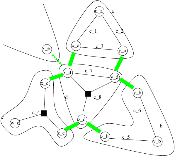
In our example, the tree structure we will use is the one shown in Figure 3(a), which also shows the direction of the child-parent relation links (via arrows). Figure 3(b) describes instead the partition of the SCSP over the four involved locations. The gray connections represent the synchronization to be assured between distinct locations. Notice that, w.r.t. Figure 2, we have duplicated the variables representing variables shared between distinct locations, because of our desire to first perform a local work and then to communicate the results to the other locations.
The scc agents (one for each location plus the parallel composition of all of them) are therefore defined as follows:
Agents ,, and represent the processes running respectively in the location , , and . Note that, at each ask or tell, the underlying soft constraint solver will only check (for consistency or entailment) a part of the current set of constraints: those local to one location. Due to the tree structure chosen for this example, where agents , , and correspond to leaf locations, only agent shows all the actions of a generic process: first it needs to collect the results computed separately by the other agents (via the ask); then it performs its own constraint solving (via a tell), and finally it can set its end flag, that will be used by a parent agent (in this case the agent corresponding to location , which we have not modelled here).
8 Conclusions and Future Work
We have shown that cc languages can deal with soft constraints. Moreover, we have extended their syntax to use soft constraints also to direct and prune the search process at the language level. We believe that such a new programming paradigm could be very useful for web and internet programming.
In fact, in several network-related areas, constraints are already being used [2, 1, 11, 17, 9]. The soft constraint framework has the advantage over the classical one of selecting a “best” solution also in overconstrained or underconstrained systems. Moreover, the need to express preferences and to search for optimal solutions shows that soft constraints can improve the modelling of web interaction scenarios.
We are indebted to Paolo Baldan for valuable suggestions.
References
- Awduche et al. (1999) Awduche, D., Malcolm, J., Agogbua, J., O’Dell, M., and McManus, J. 1999. RFC2702: Requirements for traffic engineering over mpls. Tech. rep., Network Working Group. Sept.
- Bella and Bistarelli (2001) Bella, G. and Bistarelli, S. 2001. Soft constraints for security protocol analysis: Confidentiality. In Proceedings of the 3rd International Symposium on Practical Aspects of Declarative Languages (PADL ’01), I. Ramakrishnan, Ed. LNCS, vol. 1990. Springer-Verlag, Heidelberg, Germany, 108–122.
- Bistarelli (2001) Bistarelli, S. 2001. Soft constraint solving and programming: a general framework. Ph.D. thesis, Dipartimento di Informatica, Università di Pisa, Italy. TD-2/01.
- Bistarelli et al. (2000b) Bistarelli, S., Codognet, P., and Rossi, F. 2000b. Abstracting soft constraints. In Proceedings of the 1999 ERCIM/Compulog Net workshop on Constraints, K. Apt, E. Monfroy, T. Kakas, and F. Rossi, Eds. LNCS, vol. 1865. Springer, Heidelberg, Germany.
- Bistarelli et al. (2000a) Bistarelli, S., Codognet, P., and Rossi, F. 2000a. An abstraction framework for soft constraints and its relationship with constraint propagation. In Proceedings of the Symposium on Abstraction, Reformulation and Approximation (SARA2000), B. Y. Chouery and T. Walsh, Eds. LNAI, vol. 1864. Springer, Heidelberg, Germany.
- Bistarelli et al. (1995) Bistarelli, S., Montanari, U., and Rossi, F. 1995. Constraint Solving over Semirings. In Proceedings of the 14th International Joint Conference on Artificial Intelligence (IJCAI’95). Morgan Kaufman, San Francisco, CA, USA.
- Bistarelli et al. (1997) Bistarelli, S., Montanari, U., and Rossi, F. 1997. Semiring-based Constraint Solving and Optimization. Journal of the ACM 44, 2 (Mar), 201–236.
- Bistarelli et al. (2001) Bistarelli, S., Montanari, U., and Rossi, F. 2001. Semiring-based Constraint Logic Programming: Syntax and Semantics. ACM Trans. Program. Lang. Syst. 23, 1–29.
- Calisti and Faltings (2000) Calisti, M. and Faltings, B. 2000. Distributed constrained agents for allocating service demands in multi-provider networks,. Journal of the Italian Operational Research Society XXIX, 91. Special Issue on Constraint-Based Problem Solving.
- Chen and Nahrstedt (1998) Chen, S. and Nahrstedt, K. 1998. Distributed QoS routing with imprecise state information. In ICCCCN98.
- Clark (1989) Clark, D. 1989. RFC1102: Policy routing in internet protocols. Tech. rep., Network Working Group. May.
- de Boer and Palamidessi (1991) de Boer, F. and Palamidessi, C. 1991. A fully abstract model for concurrent constraint programming. In Proceeding of the 16th Colloquium on Trees in Algebra and Programming (CAAP1991), S. Abramsky and T. Maibaum, Eds. Vol. 493. Springer-Verlag, Heidelberg, Germany.
- de Boer and Palamidessi (1994) de Boer, F. and Palamidessi, C. 1994. From Concurrent Logic Programming to Concurrent Constraint Programming. In Advances in Logic Programming Theory, G. Levi, Ed. Oxford University Press, 55–113.
- Dubois et al. (1993) Dubois, D., Fargier, H., and Prade, H. 1993. The calculus of fuzzy restrictions as a basis for flexible constraint satisfaction. In Proceedings of the 2nd IEEE International Conference on Fuzzy Systems (FUZZ-IEEE 1993). IEEE, Piscataway, NJ, U.S.A., 1131–1136.
- Fargier and Lang (1993) Fargier, H. and Lang, J. 1993. Uncertainty in constraint satisfaction problems: a probabilistic approach. In Proceeding of the 2nd European Conference on Symbolic and Quantitative Approaches to Reasoning with Uncertainty (ECSQARU1993). LNCS, vol. 747. Springer-Verlag, Heidelberg, Germany, 97–104.
- Freuder and Wallace (1992) Freuder, E. and Wallace, R. 1992. Partial constraint satisfaction. Artificial Intelligence Journal 58.
- Jain and Sun (2000) Jain, R. and Sun, W. 2000. QoS/Policy/Constraint-based routing. In Carrier IP Telephony 2000 Comprehensive Report. International Engineering Consortium, Heidelberg, Germany. ISBN: 0-933217-75-7.
- Plotkin (1981) Plotkin, G. 1981. Post-graduate lecture notes in advanced domain theory (incorporating the pisa lecture notes). Technical report, Dept. of Computer Science, Univ. of Edinburgh.
- Ruttkay (1994) Ruttkay, Z. 1994. Fuzzy constraint satisfaction. In Proceedings of the 3rd IEEE International Conference on Fuzzy Systems (FUZZ-IEEE 1994). 1263–1268.
- Saraswat (1993) Saraswat, V. 1993. Concurrent Constraint Programming. MIT Press.
- Schiex (1992) Schiex, T. 1992. Possibilistic constraint satisfaction problems, or “how to handle soft constraints?”. In Proceeding of the 8th Conference on Uncertainty in Artificial Intelligence (UAI1992). 269–275.
- Schiex et al. (1995) Schiex, T., Fargier, H., and Verfaille, G. 1995. Valued Constraint Satisfaction Problems: Hard and Easy Problems. In Proceedings of the 14th International Joint Conference on Artificial Intelligence (IJCAI’95). Morgan Kaufmann, San Francisco, CA, USA, 631–637.
..