Rounding Algorithms for a Geometric Embedding of Minimum Multiway Cut
Abstract
Given an undirected graph with edge costs and a subset of nodes called terminals, a multiway, or -way, cut is a subset of the edges whose removal disconnects each terminal from the others. The multiway cut problem is to find a minimum-cost multiway cut. This problem is Max-SNP hard. Recently Calinescu, Karloff, and Rabani (STOC’98) gave a novel geometric relaxation of the problem and a rounding scheme that produced a -approximation algorithm.
In this paper, we study their geometric relaxation. In particular, we study the worst-case ratio between the value of the relaxation and the value of the minimum multicut (the so-called integrality gap of the relaxation). For , we show the integrality gap is , giving tight upper and lower bounds. That is, we exhibit a family of graphs with integrality gaps arbitrarily close to and give an algorithm that finds a cut of value times the relaxation value. Our lower bound shows that this is the best possible performance guarantee for any algorithm based purely on the value of the relaxation. Our upper bound meets the lower bound and improves the factor of 7/6 shown by Calinescu et al.
For all , we show that there exists a rounding scheme with performance ratio equal to the integrality gap, and we give explicit constructions of polynomial-time rounding schemes that lead to improved upper bounds. For and , our best upper bounds are based on computer-constructed rounding schemes (with computer proofs of correctness). For general we give an algorithm with performance ratio .
Our results were discovered with the help of computational experiments that we also describe here.
1 Introduction
As the field of approximation algorithms matures, methodologies are emerging that apply broadly to many NP-hard optimization problems. One such approach (c.f. [8, 9, 1, 7, 6]) has been the use of metric and geometric embeddings in addressing graph optimization problems. Faced with a discrete graph optimization problem, one formulates a relaxation that maps each graph node into a metric or geometric space, which in turn induces lengths on the graph’s edges. One solves this relaxation optimally and then derives from the relaxed solution a near-optimal solution to the original problem.
This approach has been applied successfully [3] to the min-cost multiway cut problem, a natural generalization of the minimum -cut problem to more than two terminals. An instance consists of a graph with edge-costs and a set of distinguished nodes (the terminals). The goal is to find a minimum-cost set of edges whose removal separates the terminals. If the number of terminals is , we call such a set of edges a -way cut.
The first approximation algorithm for the multiway cut problem in general graphs was given by Dahlhous, Johnson, Papadimitriou, Seymour, and Yannakakis [5]. It used a traditional minimum -cut algorithm as a subroutine and had a performance guarantee of .
In the work that prompted ours, Calinescu, Karloff, and Rabani [3] used a novel geometric relaxation of -way cut in a -approximation algorithm. Their relaxation uses the -simplex , which has vertices; the vertex is the point in with and all other coordinates 0. The relaxation is as follows: map the nodes of the graph to points in such that terminal is mapped to the vertex of . Each edge is mapped to the straight line between its endpoints. The goal is to minimize the volume of ,
where cost is taken to be the cross-sectional area of edge and denotes the length of the embedded edge , defined as half the distance between its endpoints. The problem of finding an embedding that minimizes the volume can be formulated as a linear program (LP). The factor half in the length function is present to scale the distance between terminals to 1, so the LP is a relaxation of the minimum -way cut problem.
To see that the given LP is a relaxation of -way cut, consider any -way cut and let be the set of nodes reachable from terminal in the graph with the cut-edges removed. Consider a geometric embedding in which all nodes in are mapped to vertex of . For any edge, its embedded length is either 0, if the endpoints lie in the same , or 1, if the endpoints lie in distinct . Hence the volume of this embedding is equal to the cost of the -way cut.
The algorithm of Calinescu et al. finds a minimum volume embedding by linear programming. It then uses a randomized rounding scheme to extract a cut from this embedding. Ignoring the graph, the scheme chooses (from a carefully selected distribution) a -way cut of the simplex—a partition of the simplex into polytopes, each containing exactly one vertex of the simplex. The -way cut of the simplex naturally induces a -way cut in the embedded graph—namely, the set of edges with endpoints in different blocks of the partition. This cut has expected cost at most times the volume of the embedding.
1.1 Our results
Our goal is to further understand the geometric relaxation, with the hope of developing better approximation algorithms. We aim to determine the integrality gap of the relaxation and to find an algorithm whose approximation ratio matches the integrality gap. (Formally, the integrality gap is the supremum, over all weighted graphs , of the minimum cost of any -way cut of divided by the minimum volume of any embedding of . Note that the integrality gap is the best approximation ratio we can prove using an analysis that bounds the optimum cut only by the value of the relaxation.)
In this paper, we resolve this question for -cut and provide improved results for the general -cut problem. For we give a rounding algorithm with performance ratio , improving the Calinescu et al. bound of . We also show that is the best possible bound, exhibiting a graph family with a gap of between its embedded volume and minimum -way cut. Thus, for , we determine the exact integrality gap and give an optimal rounding algorithm.
For larger , we obtain results based on both computation and analysis. We give a non-constructive proof that, for every , there exists a (not necessarily polynomial time) rounding scheme whose performance guarantee equals the integrality gap. For , we use LP-derived and -analyzed rounding schemes to give explicit approximation bounds of and respectively, improving the corresponding Calinescu et al. bounds of and . For larger we give an algorithm obtaining a (analytic) bound of where . The quantity can be evaluated computationally for any fixed ; we use this to prove that for all .
Our efforts to find geometric cutting schemes that achieve good guarantees were guided by experiments: we formulated the problem of determining an optimal probability distribution on -way cuts of the simplex as an infinite-dimensional linear program and solved discrete approximations of this linear program and its dual. From these solutions we were able to deduce the lower bound and, using that, the upper bound for . These experiments also guided our search for cutting schemes that work for larger values of .
The upper and lower bounds for were discovered independently by Cunningham and Tang [4].
Presentation overview.
In Section 2 we discuss the geometric ideas underlying the problem. In Section 3 we describe the computational experiments we undertook and the results it gave for small . In Sections 4 and 5 we resolve the 3-terminal case, giving matching upper and lower bounds. Finally, in Section 6, we present our improved algorithm for general . In the appendix we prove that, for all , there exists a rounding scheme matching the integrality gap.
2 The geometric problem
Finding the integrality gap of and a rounding scheme for the relaxation turns out to be expressible as a geometric question. That is, we can express integrality gaps and algorithmic performance purely in terms of the simplex, without considering particular graphs or embeddings.
Consider an edge , which under the relaxation is embedded as a line segment in the simplex. We overload to denote this embedded segment as well. For any segment (or edge) , we let denote the projection of onto the coordinate axis, namely the one dimensional interval . We write for the minimum value in the projected interval, for the maximum value in the projected interval, and . Finally, as mentioned in Section 1, the length of an edge is defined to be half its norm, that is,
2.1 Density
Recall that a -way cut of the simplex is a partition of the simplex into polytopes, each containing a unique vertex of the simplex, and that such a cut induces a -way cut of any embedded graph. By a cutting scheme, we mean a probability distribution on -way cuts of the simplex. For any line segment , the density of on segment , denoted , is the expected number of times a random cut from cuts , divided by the length of .11 1 Note that in principle a line segment could be cut more than once by the -way cut of the simplex. We therefore speak of the expected number of times that is cut, rather than the probability that is cut.
Define the maximum density of , and the minimal maximum density as follows:
There is always a line segment of infinitesimal length that achieves the maximum density, since any segment can be divided into two edges, one of which has density no less than the original. Thus, in the remainder of this paper, we will focus discussion on such infinitesimal segments.
The relevance of is the following (this is implicit in the work of Calinescu et al.):
Lemma 2.1
For any cutting scheme and embedded graph , the expected cost of the -way cut of induced by a random -way cut from is at most times the cost of the embedding of .
Corollary 2.2
Any cutting scheme yields a randomized approximation algorithm with approximation ratio at most .
Proof: The endpoints of any edge are embedded at two points in the simplex, so the edge corresponds to a segment connecting those two points. The expected number of times the edge is cut is at most . By the Markov inequality this upper bounds the probability that the edge is cut. Thus, the expected cost of the -way cut is at most
We have already argued that lower bounds the optimum -way cut, so the result follows.
The above argument implies that no cutting scheme can have a maximum density below the integrality gap. In fact, we show that there always exists a cutting scheme whose maximum density equals the integrality gap.
Theorem 2.3
There exists a cutting scheme whose maximum density equals the integrality gap, thus, equals the integrality gap.
We give the proof in the appendix. The proof is based on the observation that the problem of choosing a rounding scheme to minimize the performance ratio is itself a (infinite dimensional) linear programming problem; furthermore its dual is the problem of choosing a weighted graph to maximize the integrality gap. This observation seems to hold in a fairly general setting beyond the -cut problem (details are in the appendix).
Calinescu et al.’s algorithm gives a cutting scheme showing that . In this paper we show that , and that, for all ,
2.2 Alignment
We have just argued that the key question to study is the maximum density of (infinitesimal) line segments relative to a cutting scheme. Calinescu et al. showed that one can restrict attention to segments in certain orientations. We say a segment in is -aligned if is parallel to the edge connecting vertices and of . We say it is aligned if it is -aligned for some pair of vertices. Calinescu et al. observed that the endpoints of any segment can be connected by a piecewise linear path of total length whose segments are aligned. The segment is cut if and only if some edge on this path is cut. Given any embedding of a graph, Calinescu et al. apply this transformation to each segment connecting two embedded vertices, without changing the volume of the embedding. Thus, they show that without loss of generality one may restrict attention to embeddings in which all edges are aligned.
Fact 2.4
Segment is -aligned if and only if and for .
(Note that denotes half the norm, while and are standard absolute values.)
2.3 Side parallel cuts (SPARCS)
In this paper, we mainly restrict attention to a particular class of cutting schemes. Define and . Note that is a hyperplane that runs parallel to the face of the simplex opposite terminal and is at distance from that face; it divides the simplex into two parts, of which is the “corner” containing terminal . An -aligned segment is cut by the hyperplane if and only if and is between and .
We define a side-parallel cut (sparc) of the simplex:
- 1.
Choose a permutation of the vertices;
- 2.
For each vertex in order by (except possibly the last), choose some ;
- 3.
Assign to vertex all points of not already assigned to a previous terminal. We say that terminal captures all these points, and that terminal cuts an edge if it captures some but not all of the yet-uncaptured part of .
This scheme cuts up the simplex using hyperplanes . In this context, we call each a slice.
We consider algorithms that sample randomly from some probability distribution over sparcs. Our restriction to sparcs was motivated by several factors. The rounding algorithm of Calinescu et al. uses only sparcs. Furthermore, our computational study of the 3-terminal problem (discussed below) and some related analytic work gave some evidence that the optimal algorithm was a distribution over sparcs (this conjecture was confirmed analytically for the 3-terminal case). Lastly, sparcs have concise descriptions (as sequences of slicing distances) that made them easy to work with computationally and analytically. It is conceivable, though, that one might do better with cuts that are not sparcs. For example, one might wish to slice off two terminals simultaneously, and then separate the two from each other. Indeed, we know of no proof that for the optimal cut must be made up of hyperplanes; curved surfaces might do better.
For segment , recall that is the interval . The key properties of sparcs are expressed in the following fact.
Fact 2.5
An -aligned segment is cut by a sparc if and only if it is cut by terminal or . Furthermore, for , the following conditions are all necessary for segment to be cut by terminal :
- (1)
- (2)
For all terminals preceding , .
- (3)
Terminal is not last in the order
For the following, let be an -aligned segment. For probability distributions on sparcs, one can obtain bounds on by using Conditions 1–3 above. For example, we can restrict our attention to Condition 1: If and are uniformly distributed over , Condition 1 holds for terminal with probability , and similarly for terminal . Thus, by linearity of expectation, the expected number of times is cut is at most .
Next, consider adding Condition 3. Suppose that the ordering of terminals is random, meaning that is last with probability . The probability that is cut by becomes , so . Thus, uniformly random ’s and a random ordering gives a performance guarantee of of , matching the bound of Dahlhous et al. [5].
To improve these bounds, one must use Condition 2. Calinescu et al. choose a sparc by selecting uniformly at random in , setting for each terminal , and slicing off terminals in random order. Conditions 1 and 3 again derive a density bound of for terminal and . Calinescu et al. improve this analysis as follows. Suppose that the edge is farther from than from . We will argue that the density contribution from terminal (i.e. the contribution to due to terminal cutting ) is only 1/2. The point is that if is such that potentially cuts , i.e. , and if (which is closer to ) precedes in the random slice ordering, then will capture all of and prevent from cutting it.
Formally, we argue as follows. Without loss of generality, assume that (note that any aligned edge can be split in two with one part closer to and one part closer to , and our assumption then applies to each part separately). As was argued before, the contribution of terminal is at most . On the other hand, with probability 1/2, precedes . If so, since , Condition 1—that —contradicts Condition 2 for —that . Thus can only be cut by terminal if precedes , in which case by Condition 1, the density contribution from is 1. Thus the density contribution from terminal is 1/2, leading to a total density of .
To improve on the 3/2 bound, we made stronger use of Condition 2. The analysis of Calinescu et al. only considers that a segment may be captured by the two terminals with which it is aligned. We derive stronger results by observing that other terminals may capture the segment as well. To do so, we had to change the cut distribution as well as the analysis. It can be shown that no distribution that holds all equal can do better in the limit than the factor of Calinescu et al. . For independent, uniformly distributed we also get the 3/2 factor. The 3/2 factor can be improved somewhat in the limit by using a non-uniform distribution on each (independent) . However, the best cutting schemes we have found are based on combining dependence and non-uniformity. One such scheme for 3-way cut gives us a bound of , which is optimal over all schemes for 3-way cut. Another scheme gives us a bound of that holds for any number of terminals. This latter scheme is designed for large ; optimizing it for smaller gives better bounds.
2.4 Additional Observations
What is the best embedding?
Perhaps the first natural question to ask is whether the embedding chosen by Calinescu et al. is the best possible.
Lemma 2.6
Among all relaxations based on embeddings in the simplex that minimize some norm (without adding other constraints) the norm has the smallest possible integrality gap.
Proof: We show that the norm maximizes the measured volume of any embedded graph; thus it minimizes the integrality gap.
Suppose we use some norm instead of the the (scaled) norm . If the norm provides a relaxation, the distance between simplex vertices must be at most one—that is, for any edge connecting simplex endpoints, we have . Consider some embedded edge . As discussed in Section 2.2, we know that under the norm it is connected by a path of aligned edges such that . Since any norm-based distance measure is translation invariant and proportion preserving, this implies that for each (which is a scaled, translated version of an edge of the simplex) we have . It follows from the triangle inequality that
Since assigns no greater a length to every embedded edge than , it also assigns no greater a volume to any embedded graph. Thus, its integrality gap is no better than that induced by the norm.
Symmetry.
A second observation is that there is no benefit in trying to identify a “good terminal order” in which to cut up the simplex.
Lemma 2.7
There is a sparc cutting scheme whose maximum density is minimum among all sparc cutting schemes and that has the following form:
- 1.
choose slice distances from some probability distribution
- 2.
apply the slice distances (in order) to a uniform random permutation of the terminals
An analogous “order independence” statement holds for the best possible (possibly non-sparc) algorithm.
Proof: For any cutting scheme , let the the corresponding “symmetrized” cutting scheme, i.e.
where varies over all permutations of .
For a line segment and a permutation , let denote the line segment obtained by permuting by the coordinates of the start point and end point of .
Then for any line segment ,
Let be the maximum density of . Then for any , the density of on is at most . The density of on is thus the convex combination of values all of which are at most , so is in turn at most . Thus the density of is no more than that of .
The above lemma shows that there is no worst-case benefit to considering specific terminal ordering. The duality argument of Section 2.1 carries over to show that a sparc with optimum expected maximum density can be specified simply as a distribution over slicing distances, without reference to an input graph embedding.
3 Our Computational Study
In this section we describe some computational experiments we carried out to help us understand the behavior of the geometric embedding. These experiments also yielded the best rounding schemes so far for the 4- and 5- terminal cut problems. One need not read this section in order to understand the following ones.
As discussed above, our goal was to find a distribution over cuts of the -simplex that minimized the density of any segment in the simplex. This problem can be formulated as an infinite dimensional linear program, with one variable per cut of the simplex, corresponding to the probability that that cut is chosen, and one constraint for every (aligned, infinitesimally small) line segment inside the simplex, which measures the expected number of times the chosen cut will cut that segment. Of course, it is not tractable to solve the infinite LP computationally, but we expected that discretized versions of it would be informative.
We applied this approach in two distinct ways. For the 3-terminal case, we devised an LP that exploited the planarity of the 3-terminal relaxation to home in on a “worst case” embedded graph. By examining this graph, we were able to deduce requirements for the optimal algorithm, which led to its identification. For the general case, we devised an LP whose solutions are (provable) upper bounds on the performance of certain rounding algorithms. We solved this LP for small numbers of terminals (3–9), deriving algorithms with (computer aided) proofs of the best known performance ratios for these problems. The solution suggested certain properties that appear to hold in the “optimal” rounding scheme; we used these suggestions in our development of (analytic) solutions for arbitrary numbers of terminals.
3.1 The three-terminal case
For the -terminal problem we exploited planarity. The 3-simplex can be viewed as a triangle in the plane. We discretized the linear program by defining a triangular mesh over the simplex and considering only edges of the mesh instead of all line segments in the simplex. A (rather coarse) example mesh is shown in Figure 1. Note that we have augmented the triangular mesh with rays starting at the corners of the simplex and heading out to infinity.
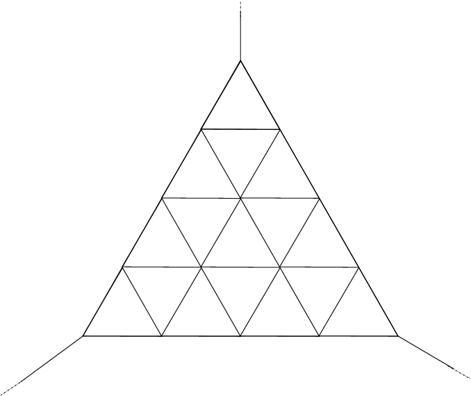
We used the planarity of the 3-simplex to simplify our LP formulation. The planar dual of the augmented mesh is shown in Figure 2. Note that because of the augmentation, the dual has three auxiliary nodes , , and corresponding to infinite regions of the primal, one node for each side of the simplex.


Any minimal 3-way cut of the mesh corresponds to a collection of two or three paths (representing the boundary of the cut) through the planar dual of the augmented mesh. Specifically, the cut corresponds to either
- 1.
two paths whose endpoints are the nodes , , and (illustrated in Figure 3), or
- 2.
three paths all originating at some interior dual node and terminating at the nodes , , and (illustrated in Figure 4).
Given an assignment of weights to the edges of the mesh, the weight of the minimum 3-way cut of the first type is
and the minimum 3-way cut of the second type is
To find an embedded graph that is “worst-case” (up to the discretization), we solve a linear program that has a weight variable for each edge of the triangular mesh (not including the rays). The linear program also has a distance variable for every pair of nodes of the dual (including auxiliary nodes). The objective is to minimize the total weight subject to the condition that every 3-way cut has value at least 1. This condition can be expressed by a collection of constraints on distances through the dual graph.
Using the above linear program, we first deduced the general form of the dual solution, giving us the lower bound for . From this we deduced the necessary structure of any optimal primal solution (using complementary slackness conditions), including the important idea of “ball cuts” versus “corner cuts” which we will discuss in the following sections.
3.2 The general case
In the general case, the lack of a planar embedding prevented us from exploiting nice properties of its cuts; we were faced with the problem of enumerating cuts as well as edges. Based on the work of Calinescu et al. and our own results for the optimal 3-terminal solution, we decided to limit our exploration to sparcs as discussed above.
There is still an infinite space of possible sparcs, so we discretized our problem. Fix an integer grid size . A discrete sparc is described by a vector where each is an integer in the range . Given such a vector, we choose a random sparc by setting uniformly in the range . This defines a probability distribution on sparcs. We now define a linear program to search for a probability distribution over all discrete sparcs (which induces a probability distribution over all sparcs). We define a variable for each discrete sparc, which reflects the probability of choosing that discrete sparc, and provide constraints that upper bound the density of every possible segment under this probability distribution. We then aim to minimize the largest of these densities.
There are infinitely many segments, but we define a finite set of constraints that allow us to upper bound the density of all of them, as follows. The slices at distances () for each terminal partition the simplex into cells
For a given distribution on the discrete sparcs, we can compute a (linear) upper bound on the density induced on any segment with a given alignment within a cell, and specify one constraint saying that this upper bound should be small. Since the cells are small, we expect all segments with a given alignment to have roughly the same density under our cutting scheme, so we hope that the upper bound is reasonably tight. With this simplification, the number of constraints is bounded by the number of cells times the number of segment alignments per cell, which is at most .
We determine the upper bound for a cell as follows. For any discrete cut, the slices generated from it will fall into one of three categories. If the coordinate of the discrete cut is different from that of the cell, then the slice will not pass through that cell: depending on whether the coordinate is larger or smaller it will either capture the entire cell or none of the cell. If the coordinates are the same, then the slice might pass through the cell; we can use the fact that the slice is uniformly distributed over a range to determine its density contribution.
An -aligned segment can only be cut if the slices for terminal or go through its cell (and no earlier slice captures the entire cell). If only one of the two slices goes through the terminal then its contribution to a segment’s density is at most (the length of the segment divided by the width of the cell). If both slices go through the cell, their contribution is at most . We ignore the fact that different slices within the cell might capture the segment before it can be cut, thus introducing some slack in our upper bound.
In view of Lemma 2.7, we need only represent cutting schemes that consider terminals in random order. Recall that each assignment of integers in to defines a discrete sparc. We let be the variable assigning a probability to this sparc in the cutting scheme. For any permutation of , the probability of applying this sparc to the sequence of terminals is .
In order to present the linear program, we require a bit of notation. For (the ’s representing a discrete sparc and the ’s representing a cell), for a permutation of , and for , define
The value of is 0 if some slice earlier than the slice for terminal captures the cell defined by .
Define to be 1 if and zero otherwise.
The linear program minimizes subject to the following constraints.
| (1) |
| (2) | |||||
| (3) |
We can exploit symmetry to further reduce the number of constraints we consider. Since by assumption our sparc slices terminals in random order, two segments that are identical under permutation of coordinates will have the same densities, so we need consider only one of them. Thus, we restrict our constraints to -aligned segments in which the remaining coordinates are in nondecreasing order. For each such segment and cell, we use one constraint to measure the average density induced by a given sparc over all permutations of the terminal orders.
3.3 LP Results
Exploiting symmetry as discussed above, we were able to solve relatively fine discretizations of the problem. We wrote a simple program to generate the linear programs automatically, and used CPLEX to solve them. While it is difficult to “prove” programs correct, our computations did converge to the correct approximation ratio for the 3-terminal case.
We give our results below in tabular form. We derived improved bounds for – terminals. Note that these programs optimize a proven upper bound on the approximation ratio; thus,under the assumption that the programs were correct, these numbers are proven upper bounds. In fact, since the programs output a particular distribution over discrete cuts, their performance ratio could be proven analytically via a tedious case analysis on each cell of the discretize grid (which we have not performed).
| grid size | corner cut probability | bound | ||
|---|---|---|---|---|
| 3 | 90 | .284 | 1.0941 | 1.167 |
| 4 | 36 | .289 | 1.1539 | 1.250 |
| 5 | 18 | .314 | 1.2161 | 1.300 |
| 6 | 12 | .376 | 1.2714 | 1.333 |
| 7 | 9 | .397 | 1.3200 | 1.357 |
| 8 | 6 | .414 | 1.3322 | 1.375 |
Our experiments also revealed one interesting fact: in all cases, the optimum cut distribution made use of “corner cuts.” That is, the output distribution had the following form: with some probability, place each slice at a distance chosen uniformly between 0 and from its terminal; otherwise, use a (joint) distribution that places every slice at distance greater than from its terminal.
Adding constraints that forced the corner cuts to operate over a range other than 1/3 of the way from the terminals worsened the computed performance ratio, hinting that perhaps the optimal algorithm uses corners of size exactly 1/3. This result is consistent with the optimal 3-terminal algorithm, but inconsistent with the corner cut placement in the analytical solution for higher that we give later. We may be observing a misleading artifact of working with a small discretized problem, or we may be missing something in our analytic solution.
4 Upper Bound for
Our analytic upper bound of for comes from a new cutting scheme that we call the ball/corner scheme. Though for simplicity we present a non-sparc scheme, there is a similar scheme using sparcs that achieves the same bound.
For , the simplex can be viewed as a triangle in the plane, which simplifies our pictures. However, we continue to use the original three-dimensional coordinate system to locate points in the simplex. Our cut of the simplex is determined by some lines and rays drawn through the triangle; we refer to them as boundaries. We will show that no segment has high density with respect to our random choice of boundaries.
As illustrated in Figure 5, number the vertices of the simplex and . Let points divide the edges in thirds, so that –––––– is the hexagon in with side length22 2 Remember that we measure length as half the norm. , with side – on the side of the triangle connecting terminals and . Note that this hexagon is (a scaled version of) the unit ball for our distance metric. The points on the boundary of the hexagon are each at distance from the hexagon’s center.Outside the hex, we have a corner for each terminal consisting of the points with .
4.1 The Ball/Corner Scheme
The ball/corner scheme chooses a ball cut with probability , otherwise it chooses a corner cut. These two types of cuts are defined next. The scheme is illustrated in Figure 5.
Ball cut: Choose a point uniformly at random from either line – or line –. Consider the three lines () parallel to the triangle’s sides and passing through the point . Each such line is divided at the point into two rays. Thus we get six rays. Each side of the triangle intersects two of these rays. For each side, choose uniformly at random one of the two rays that hit it. This gives three rays; they form the boundary of the -way cut. (For a sparc-based equivalent of this algorithm, we can choose (in random order) two of the three sparcs that pass through the chosen point .)
Corner Cut: Choose two terminals in , and a value , uniformly at random. For each of the two chosen terminals , let . The two lines form the boundaries of the -way cut. (Note that a corner cut is a sparc.)
4.2 Analysis
We first state two simple properties of the ball cut that we need to analyze the performance of the cutting scheme:
Fact 4.1
Each of the coordinates of the random point is uniformly distributed in .
Fact 4.2
Once is chosen, each one of the six candidate rays connecting to one side of the triangle is chosen with probability .
Theorem 4.3
The maximum density of the ball/corner scheme is , so .
Proof: We show that the expected density of any segment is at most . For the ball cuts, we use only the two facts claimed above. Since these two facts, as well as the corner cut scheme, are symmetric with respect to the three coordinates, it suffices to prove the claim only for a -aligned segment . Further, we may assume assume that is entirely contained in either a corner or the hex; for otherwise, as discussed in Section 2.1, we can just split into corresponding pieces, calculating the density for each piece separately. We will consider several cases, depending on where is located.
First, assume is located entirely in the hex. Such a segment cannot be cut by a corner cut, so we need only consider the density when a ball cut is made and multiply by the probability of choosing a ball cut, namely . Assume a ball cut is made. Then can only be cut by rays in for . By Fact 4.1, is uniformly distributed in . Hence, the probability that goes through is since is -aligned. If touches , it is at a single point. By Fact 4.2, the ray of containing this point is picked for the cut with probability . Thus the expected number of times is cut is .
Exactly the same argument applies if the edge is in the corner closest to terminal . The ball cut contributes the same density, while the corner cut contributes nothing (note that a -aligned edge is parallel to the line , so cannot be cut by it).
Finally, suppose segment is in the corner closest to terminal (a symmetric argument applies if is in the corner closest to terminal ). In this case, if a ball cut is made, the above analysis applies except that only the line can cut (the line never enters the corner), so the density contribution of the ball cut is halved to . But the edge can also be cut by a corner cut. A corner cut is chosen with probability . When it is, two of the three terminals are chosen, so terminal is chosen with probability . If terminal 1 is chosen, then, since the cutting line near terminal 1 is of the form , where is chosen uniformly in , the probability that the line cuts is . Thus, the expected number of times that the edge is cut (by a ball cut or corner cut) is .
5 Lower Bound for
Theorem 5.1
For , the minimum maximum density . Hence, the integrality gap for the geometric relaxation is .
Note that this theorem applies to all cutting schemes, not just sparcs. Thus, the scheme of the previous section is optimal.
Proof: Fix to be any positive integer. We construct an embedded weighted graph with no 3-way cut of cost less than , but with an embedding of cost . This immediately demonstrates an integrality gap of . Furthermore, it implies that no cutting scheme has maximum density less than , because by Lemma 2.1 such a cutting scheme applied to would yield a -way cut with expected cost less than , a contradiction. Since is arbitrary, the result follows. Our construction (for ) is shown in Figure 6.


For any pair of distinct terminals and number , define embedded path as follows. Let be the terminal in , let be the point on segment at distance from , and let be the point on segment at distance from . Then is the union of the three segments , , and .
We form the graph from paths for , where is an integer multiple of . Although we describe the graph as a set of paths, technically it is a planar graph consisting of nodes and edges as follows: for every point in whose coordinates are integer multiples of , there is a node in the graph embedded at that point; for every pair of nodes embedded units apart, has an edge with cost equal to the number of paths that pass through both nodes.
With this understanding, we now specify the graph. For each of the distinct pairs of terminals , there are paths. Of these paths, run directly between the terminals; that is, there are copies of . The remaining paths are the paths where .
The total cost of the embedding is the total length of the paths. Since a path has length , a direct calculation shows that the total length of the paths is .
Next we lower bound the cost of any 3-way cut. Since the graph is planar, any minimal 3-way cut corresponds either to a disconnected cut (meaning that the cut is the union of two disjoint 2-way cuts, each separating some terminal from both other terminals), like our upper bound’s corner cut, or a connected cut (meaning that the cut edges give, in the planar dual, three paths connected at some central node and going to the three sides of the triangle), like our upper bound’s ball cut.
Any 3-way cut must cut all of the paths at least once. To finish the proof, we will argue that for either type of 3-way cut (connected or not), at least paths are cut twice, so that the edges cut by the 3-way cut cost at least . This is easy to verify for a disconnected cut: a disconnected cut is the union of two 2-way cuts, so the paths running between the two terminals that are cut off must be cut twice.
Now consider any connected cut. In the planar dual of , the connected cut corresponds to a central node and three paths from the node to each side of the triangle. Let be any point inside the face of corresponding to the central node. Consider a path such that , where . That is, is inside the cycle formed by the union of and . Then the path is cut at least twice by the connected cut. For fixed and , the number of such paths (with ) is . Thus, the total number of such paths is more than .
6 Improvement for general
We now present an algorithm for an arbitrary number of terminals. While this algorithm seems unlikely to be the best possible, it improves on the previous best bound. As discussed in Section 2.3, the essential observation in this analysis is that many slices can capture an edge before it has a chance to be cut.
Theorem 6.1
For all , . Moreover, there is a -way cut randomized approximation algorithm with an approximation guarantee of .
Our bound improves on the Calinescu et al. bound of for all . For , we show that by specializing the analysis for small (see Subsection 6.1).
To prove the theorem, we will use a (sparc) cutting scheme, that is,
we choose slicing thresholds , and apply the slices
to a random permutation of the
terminals. We are going to apply either an independent cut (ICUT) or
a corner cut:
ICUT: each is chosen independently and
uniformly in .
Corner cut: all are chosen equal to a
single random picked uniformly in .
We will apply ICUT with probability
and apply a corner cut with the remaining probability.
Before proving that the above sparc achieves a maximum density below 1.3438, as in Theorem 6.1, let’s first draw parallels to our scheme for . The corner cut is completely analogous, except that is now chosen in the interval instead of . However, ICUT is very different from the ball cut. For example, the are now independent whereas they were highly dependent in the ball cut. The reader may wonder why we did not just generalize the ball/corner cut scheme. However, corner cuts are only meaningful for since this is the region in which the are disjoint. On the other hand, the maximal ball of the -simplex has center and radius . Already for , the simplex cannot be covered by a ball and corners, and for large, the measure of the ball is vanishingly small. Hence, the concept of ball cuts is not really relevant for large .
To bound the cutting density of our scheme, we will bound the density of every segment. As justified in Section 2.2, we consider a segment of length , and let approach zero. As in the ball/corner scheme, by symmetry we can assume without loss of generality that the segment is -aligned.
Define to be the density with which ICUT cuts a -aligned segment of infinitesimal length located at . We will show:
Lemma 6.2
By Lemma 6.2, this combined scheme gives a density of for non-corner segments (since they are cut only if ICUT is used, and then only with probability 2.014096), and a density of for corner segments (combining their probabilities of being cut by the two schemes), for a maximum density of , proving Theorem 6.1. To finish the proof of Theorem 6.1, it remains only to prove Lemma 6.2.
ICUT’s cumulative probability distribution function for any is . The corresponding probability density function is
Consider a -aligned segment of length with one endpoint fixed at . As goes to zero, the density of this segment goes to
| (4) |
where the sum is over all orderings of the terminals. This formula follows from Fact 2.5. The first term measures the probability that the segment is cut by terminal 1, which happens if the slice for terminal 1 goes through the segment while all slices preceding terminal 1 in the ordering fail to capture the segment. The second term similarly measures the probability that the segment is cut by terminal 2. Considering the slices for terminals other than 1 and 2 is the crucial element in improving the density bound of 3/2 for large . The formula assumes that is continuous around each and that is continuous in an open region around and . The latter is not the case around . However, as discussed Section 2.1, we may assume that all segments considered have been subdivided so that for each , either or .
Note that (provided ), because implies terminal cannot save the edge. Note also that is symmetric with respect to the variables for . Define
In these definitions, is required to lie in the -simplex.
is the maximum density of any -aligned infinitesimal segment with an endpoint whose first two coordinates are . Note that the maximum is well-defined and achieved by some because the simplex is closed under limits.
To understand ICUT, our first goal is to characterize . We consider as it is one candidate for .
Lemma 6.3
for all .
Proof: .
Thus for fixed , is a nondecreasing sequence bounded from above (by 2). This implies that is well-defined. We will see later that is also well-defined.
Next we show that for fixed and , the maximum for occurs at either the “central point” or the “three-terminal” point .
Lemma 6.4
Proof: Fix and . Let .
Claim 1: Among all such that for all (and is in the simplex), the unique maximizer of satisfies , so is equal to . Suppose for contradiction that some other such maximizes . Then for some . Considered just as a function of and (holding the other coordinates fixed)
| (5) |
where , , and are nonnegative and independent of and . Furthermore because is symmetric in and . Consider increasing and decreasing at equal rates. This maintains but increases at a rate proportional to
This is positive because for and (recall that ). This contradicts the choice of .
Claim 2: Among all such that for some (and is in the simplex), the unique maximizer of satisfies and for , so is equal to . Suppose for contradiction that some other such maximizes . Fix some such that . Since by assumption , we have and thus the expression (5) reduces to . If we increase and decrease at the same rate, the rate of increase in is , contradicting the choice of .
The two claims together prove the lemma.
Lemma 6.5
For , .
An immediate corollary is that is well-defined and for all . Using this and Lemma 6.4, to bound it suffices to bound and . We begin with .
Lemma 6.6
Proof: Fix and . Our first goal is to derive a closed-form expression for for any . Fix for now and let for .
For , let denote the probability that the segment at is not captured by a terminal other than before terminal ’s cut is made:
Then .
We will derive a closed-form expression for (and by symmetry for ). Recall that for . We thus rewrite
Here we condition on , the number of such that . Note that is uniform in while is the probability that , given . A change of variables and rewriting give
Now we let . The two sums above have standard closed forms that tend respectively to
where . Thus, as ,
Of course tends to the above with replacing . This gives us our closed-form expression for :
| (6) |
where .
The above equality holds for any suitably well-behaved . Using this closed form and our particular choice of , we now show the two desired bounds on .
Case 1:
. In this case , , and . So (6) gives
where so . Let . In the rest of this case (Case 1), we will prove that for . The cases and follow by the continuity of . The claim is “obvious” from a plot but the somewhat technical proof appears below.
We show that is strictly concave for . It therefore has a unique maximum at some , where . By substitution, and , so . Hence
To show is strictly concave, we show that is strictly negative. Now,
and
To show that is negative, it suffices to prove that
is negative. By substitution, and , so it suffices to show that has only one zero , for and for . Here
and . For , has only one zero and for and for . That is, is first decreasing and then increasing. Since and it follows that has only one zero for .
Case 2:
or . Assume (the case is symmetric). In this case, and , so we get
As before, let . We will prove that for . First, , so follows if we can show that for . We have
Define . Since for , if and only if . Since , we can infer if for all . We have . Note that , so follows if for . We have , so . We conclude that if .
Lemmas 6.4 through 6.6 prove that, for such that for all ,
The remaining case is when for some . In this case by Lemma 6.4,
and . Thus, to finish the proof of the theorem, it suffices to show the following lemma.
Lemma 6.7
If , then
Proof: Let .
Then while , , and .
By inspection of (4), .
This proves Lemma 6.2.
6.1 Improvements for small values of
For particular values of it is possible to refine the analysis in the proof of Theorem 6.1 to get improved bounds. In this case it is useful to modify the algorithm so that it only uses cuts instead of . In particular, we do not use the cut for the terminal with . The analysis for this modified algorithm goes similarly, with our definitions appropriately modified to reflect that we are using instead of cuts.
Then, instead of passing to the limit, can be evaluated directly. Following this approach we obtained the following performance guarantees for particular :
| corner placement | ICUT probability | bound | |
|---|---|---|---|
| 3 | .641 | .675 | 1.131 |
| 4 | .607 | .663 | 1.189 |
| 5 | .588 | .659 | 1.223 |
| 6 | .576 | .659 | 1.244 |
| 7 | .565 | .657 | 1.258 |
| 8 | .557 | .656 | 1.269 |
| 9 | .557 | .659 | 1.277 |
| 10 | .557 | .661 | 1.284 |
| 12 | .554 | .661 | 1.293 |
| 20 | .554 | .666 | 1.314 |
| 35 | .550 | .666 | 1.327 |
“Corner placement” is the placement of the corner (analogous to ) and “ICUT probability” is the probability of choosing ICUT. These parameters were chosen to try to minimize the resulting bound on the performance ratio, shown under “bound”. These numbers are approximate; the ratios were evaluated numerically without formal verification.
7 Conclusion
We have provided a better analysis of an embedding relaxation for multiway cut. We have exactly determined the integrality gap for the 3-terminal problem, and given an approximation algorithm achieving the bound. For larger values of , we have defined a class of cutting schemes called sparcs that, through a combination of nonuniform and dependent rounding, provide better approximation ratios than the best previous schemes. However, the question of the exact integrality gap remains open.
References
- [1] Yonatan Aumann and Yuval Rabani. An approximate min-cut max-flow theorem and approximation algorithm. SIAM Journal on Computing, 27(1):291–301, February 1998.
- [2] Patrick Billingsley. Probability and Measure, 1995. John Wiley & Sons.
- [3] G. Calinescu, H. Karloff, and Y. Rabani, “An improved approximation algorithm for Multiway Cut”, Journal of Computer and System Sciences, 60(3): 564–574, 2000.
- [4] W. H. Cunningham and L. Tang, “Optimal 3-terminal cuts and linear programming,” Proceedings of the Seventh Conference on Integer Programming and Combinatorial Optimization (IPCO), Lecture Notes in Computer Science1610, Springer-Verlag, pages 114-125, 1999.
- [5] E. Dahlhaus, D. S. Johnson, C. H. Papadimitriou, P. D. Seymour, and M. Yannakakis. The complexity of multiterminal cuts. SIAM Journal on Computing, 23(4):864–894, August 1994.
- [6] Guy Even, Joseph (Seffi) Naor, Satish Rao, and Baruch Schieber. Divide-and-conquer approximation algorithms via spreading metrics Journal of the ACM, 47(4): 585–616, July 2000.
- [7] Michel X. Goemans and David P. Williamson. Improved approximation algorithms for maximum cut and satisfiability problems using semidefinite programming. Journal of the ACM, 42(6):1115–1145, November 1995.
- [8] F. T. Leighton and S. Rao. Multicommodity max-flow min-cut theorems and their use in designing approximation algorithm Journal of the ACM, 46(6): 787–832, 1999.
- [9] Nathan Linial, Eran London, and Yuri Rabinovich. The geometry of graphs and some of its algorithmic applications. Combinatorica, 15(2): 215–245, 1995.
8 Appendix
Proof of Theorem 2.3.
We show that there necessarily exists a cutting scheme whose maximum density equals the integrality gap of the relaxation. The basis of this proof is that the two quantities are solutions to dual linear programs. Although the linear programs are infinite, we show they have no duality gap.
Interestingly, most of the proof holds in the following more general setting: We have a non-negative real vector representing a relaxed solution to some problem. There is a set of allowable solutions (also nonnegative real vectors), and we want to round to some solution . The method for rounding is represented by a randomized rounding scheme, which is simply a probability distribution on .
We assume that the cost of is given by for some nonnegative weight function , and likewise the cost of any is . We want to choose a single rounding scheme that has a good performance ratio against all possible weight functions . (We will see that this is analogous to choosing a single rounding scheme of the simplex that has good performance ratio against all embedded graphs.)
Define the performance ratio of a rounding scheme to be
(This corresponds to the maximum density of a cutting scheme.) Here the notation signifies the expectation over chosen according to the probability distribution .
Define the integrality gap to be
the worst-case ratio of the minimum-cost of any true solution to the cost of the relaxed solution.
Lemma 8.1
The performance ratio can be reformulated as
In the case of k-cut, each index corresponds to a “seglet” (edge of the divided simplex), and corresponds to an embedded graph ( corresponds to the number, or total weight, of edges embedded along seglet ). In that case the lemma says that, to check the performance guarantee of a rounding scheme, it suffices to check it for each seglet.
The proof is similar to the observation regarding two-player zero-sum matrix games that once one player has fixed their mixed strategy, the other player has an optimal mixed strategy that is pure.
Proof: Clearly the left-hand side is greater than or equal to the right-hand side (take to be any of the unit vectors with a single coordinate equal to 1 and the others 0). To finish we show that the left-hand side is at most the right hand side for any fixed .
Fix . Let equal the right-hand side above. Note that by linearity of expectation, the left-hand side is
By the definition of , , so the quantity above is at most
Theorem 8.2
If and the dimension of are finite, then there exists a rounding scheme whose performance ratio equals the integrality gap.
Proof: Let be the probability that we choose solution . Choosing an optimum rounding scheme is equivalent to the following linear program:
The dual of this program is
By the change of variables , this is equivalent to
But it is easy to verify that this is equivalent to the problem of choosing a weight function to achieve the integrality gap. If and the vectors in are finite-dimensional and is finite, then strong duality implies that the linear programs have equal values.
Next we describe how this relates to the rest of the paper. Define edge set to be all edges (pairs of points) in the simplex. Define for . Define to contain the characteristic vectors of -way cuts of the simplex: if is cut by and 0 otherwise. An embedding of a particular weighted graph in the simplex then corresponds to a particular weight function , where equals the total weight of edges embedded on simplex edge . With this , , and interpretation of , we have the following correspondences:
| general setting | -way cut | |
|---|---|---|
| embedded | ||
| -way cut of | ||
| cost of -way cut of | ||
| rounding scheme | cutting scheme | |
| performance ratio of | ||
| integrality gap | integrality gap |
Thus, if and the dimension of were finite, we could conclude by the theorem that the equals the integrality gap of the relaxation. This yields an immediate corollary:
Corollary 8.3
For input graph instances of any bounded size, there is a rounding scheme whose performance is equal to the integrality gap of the relaxation.
Proof: Consider the set of all graphs whose size is bounded by some quantity. Each has a bounded number of vertices, and the (rational) weights on the graph are also of bounded size. The linear programming relaxation thus also has bounded size. It follows that any vertex solution to the linear programming relaxation, which assigns embedding coordinates to all the vertices, has bounded size—meaning that the coordinates are rational numbers of bounded size. The set of coordinates at which vertices might be located in an optimal embedding therefore forms a discrete grid within the simplex, with a finite number of points. The embedded edges connect these points, so there is a finite number of embedded edges in the optimal solution. An input instance is determined entirely by the weights assigned to these edges, so has finite dimension. Similarly, for the purposes of rounding we need only consider -way partitions of the finitely many grid vertices. There are only finitely many of these partitions.
Since the dimension of inputs and the number of output solutions is finite, the previous theorem applies and shows that there is a rounding scheme with performance equal to the integrality gap of the embedding.
If we want a rounding scheme that works (uniformly) for graphs of arbitrary size, we have to work somewhat harder. Wee show that the desired result follows as a limiting case of Theorem 8.2.
In what follows, we restrict the -way cut problem to various particular subsets of the edge set of the simplex. A -way cut of is defined to be a subset of such that contains no terminal-to-terminal path By the minimal maximum density with respect to we mean
where ranges over cutting schemes of (probability distributions over -way cuts of ). By the integrality gap with respect to we mean
where ranges over weight functions on with finite support.
Our goal is to show . Since we know , it suffices to show .
Define to contain those edges in with rational endpoints. (In fact, any countable dense set will do in place of the rationals.) Fix any enumeration of the edges in . Let set contain the first edges in the enumeration. It suffices to show the following equality:
| (10) |
because by Theorem 8.2 we know , and clearly , so combining with (10) proves the theorem via
Thus, to prove Theorem 2.3, we need only prove (10). In the remainder of the section we prove it as follows: We first show we can extend any sequence of cutting schemes, one for each , to a single good cutting scheme for their union (edges with rational endpoints). This shows . We then show that we can extend the cutting scheme on to a cutting scheme on (all edges). This shows .
One measure-theoretic issue that we must first address is how we formally define a probability distribution on our infinite sets and . For this we use Kolmogorov’s Existence Theorem [2, ch. 7].
Before we explain, we introduce some terminology. Note that any cutting scheme of a set induces a cutting scheme on each subset by restriction. We say that any from which can be so obtained is consistent with .
Kolmogorov’s Existence Theorem implies the following. Fix any . Consider a family of cutting schemes of the finite subsets of . If this family is consistent, meaning that whenever two cutting schemes and in the family satisfy , the second scheme is consistent with the first one, then there exists a single cutting scheme of , with consistent with each in the family.
In this section, to describe any cutting scheme on (or ), we specify the consistent family of cutting schemes it induces on the finite subsets. The following lemma gives a useful condition for the existence of such a family. We will use it twice.
Lemma 8.4
Let be any subset of . Suppose there exists a sequence of cutting schemes that converges in the following sense: for each finite and each -way cut of , the limit
| (11) |
is well defined. Define to be the cutting scheme of that, for each -way cut of , chooses with probability in (11), i.e. . Then is a consistent family of cutting schemes, so by Kolmogorov’s Existence Theorem there exists a cutting scheme of consistent with each .
Proof: We need to verify the following:
- 1.
Each is a cutting scheme: with each , where ranges over all cuts of .
- 2.
For and with both finite, is consistent with . That is, for any cut of ,
where ranges over all -way cuts of such that .
In each case, the desired property holds for the cutting scheme induced on (and/or ) by for large enough . For example, to verify the second property, use
The first equality is by definition of , the second is because the finite sum of the limits is the limit of the sums, and the last is because, for large enough, the term inside the limit is well defined and necessarily 0 (simply because is a cutting scheme, so the induced cutting schemes and are necessarily consistent). The first property follows similarly.
We need one last “utility” lemma. It will help us construct a sequence of cutting schemes that converges in the sense needed for Lemma 8.4.
Lemma 8.5
Consider a countable collection of countable sequences of real numbers, where each sequence in lies in some finite interval .
Then there exists an infinite index set such that for each sequence , the limit
is well defined.
Proof: The proof is a “dovetailing” variation of the standard proof that any sequence in a compact set contains an infinite convergent subsequence.
Order the sequences arbitrarily and consider the infinite matrix whose th row is the th sequence. Associate with each sequence an interval , initially . Visit the sequences in the standard dovetailing order; that is, visit the th sequence for each , so that each sequence is visited infinitely often.
While visiting a sequence , narrow the associated interval to either its upper or lower half, and then delete from the matrix all the columns such that is no longer in the associated interval. Further, make the choice of upper or lower half so that infinitely many columns remain undeleted. (This is possible because each of the infinitely many ’s lying in a column that was previously not deleted lies in one of the two halves.)
To complete the construction, define to be the smallest index larger than of any column that remains undeleted after the th step of the construction, and take . It is easy to verify that for each , the subsequence converges.
Now we can begin our two-step proof that . First we show that if each has a good cutting scheme, then there is an equally good cutting scheme of .
Lemma 8.6
There exists a cutting scheme of with maximum density . Thus,
Proof: Let . Say a sequence of cutting schemes is good if each is a cutting scheme of and has maximum density at most with respect to . By the definition of , there exists a good sequence of cutting schemes .
Consider each pair where is a finite subset of and is a cut of . Since there are only countably many such pairs, Lemma 8.5 implies that there exists an infinite index set such that, for each pair ,
is well-defined. By Lemma 8.4, each is a cutting scheme and there exists a cutting scheme of that is consistent with each .
It remains to verify that has maximum density with respect to . Observe that, for any edge and any cutting scheme , is a cutting scheme that chooses among at most two cuts, the set itself and (possibly) the empty set, and that the probability that chooses the set is the probability that chooses some cut that contains .
For any edge ,
Hence, for any edge , the probability that cuts is at most .
Lemma 8.7
Let be the cutting scheme of of maximum density (shown to exist in Lemma 8.6). There is a cutting scheme of that has maximum density with respect to . Thus .
Proof: For each point in the simplex, fix a sequence of rational points converging to . For any set , let denote .
Define a sequence of cutting schemes of by . That is, maps each real point to its th rational approximation, then cuts using a random cut from . We claim that for each finite and each cut of , the limit
is well defined.
To show the claim, it is enough to show that for all , for all large enough and . Let and . By consistency,
where ranges over all the cuts of other than that are consistent with . Each of the cuts that takes on cuts at least one of the segments where ranges over the endpoints of the edges in , so the corresponding term in the sum is at most . Since there are finitely many terms and is finite and , it follows that the sum on the right is arbitrarily small for large enough and . Thus (and likewise ) tends to zero for large and . Thus so does . This proves the claim.
Define . By Lemma 7.4, there is a cutting scheme of that is consistent with each . The argument used at the end of the proof of Lemma 8.6 shows that, for any edge ,
Thus the maximum density of is at most .