{bottomstuff}

This work was supported by the Ministry of Education, Science and Sport of Slovenia, Project J1-8532. It is a detailed version of the part of the talk presented at Recent Trends in Graph Theory, Algebraic Combinatorics, and Graph Algorithms, September 2001, Bled, Slovenia.

Generalized Cores

VLADIMIR BATAGELJ and MATJAŽ ZAVERŠNIK
University of Ljubljana FMF Department of Mathematics
and IMFM Ljubljana Department of TCS
Jadranska 19 1000 Ljubljana Slovenia

Received R

Abstract

Cores are, besides connectivity components, one among few concepts that provides us with efficient decompositions of large graphs and networks. In the paper a generalization of the notion of core of a graph based on vertex property function is presented. It is shown that for the local monotone vertex property functions the corresponding cores can be determined in $O(m\max(\Delta,\log n))$ time.

Keywords:

Algorithms, Performance, Theory

keywords

Computations on discrete structures

keywords

algorithm, decomposition, generalized cores, large networks

1 Cores

The notion of core was introduced by Seidman in 1983 [6, 7].

Let $\mathbf{G}=(V,L)$ be a simple graph. $V$ is the set of vertices and $L$ is the set of lines (edges or arcs). We will denote $n=|V|$ and $m=|L|$ . A subgraph $\mathbf{H}=(C,L|C)$ induced by the set $C\subseteq V$ is a $k$ -core or a core of order $k$ iff $\forall v\in C:\deg_{H}(v)\geq k$ and $\mathbf{H}$ is a maximum subgraph with this property. The core of maximum order is also called the main core. The core number of vertex $v$ is the highest order of a core that contains this vertex. Since the set $C$ determines the corresponding core $H$ we also often call it a core.

Refer to caption — Figure 1: *0, 1, 2 and 3 core*

The degree $\deg(v)$ can be the number of neighbors in an undirected graph or in-degree, out-degree, in-degree $+$ out-degree, … determining different types of cores.

The cores have the following important properties:

•

The cores are nested: $i<j\ \ \Longrightarrow\ \ \mathbf{H}_{j}\subseteq\mathbf{H}_{i}$
•

Cores are not necessarily connected subgraphs.

In this paper we present a generalization of the notion of core from degrees to other properties of vertices.

2 $p$ -cores

Let $\mathbf{N}=(V,L,w)$ be a network, where $\mathbf{G}=(V,L)$ is a graph and $w:L\to\hbox{\sf I\kern-1.4pt\hbox{R}}$ is a function assigning values to lines. A vertex property function on $\mathbf{N}$ , or a $p$ function for short, is a function $p(v,U)$ , $v\in V$ , $U\subseteq V$ with real values.

Examples of vertex property functions: Let $N(v)$ denotes the set of neighbors of vertex $v$ in graph $G$ , and $N(v,U)=N(v)\cap U$ , $U\subseteq V$ .

1.

$p_{1}(v,U)=\deg_{U}(v)$
2.

$p_{2}(v,U)=\mbox{\rm indeg}_{U}(v)$
3.

$p_{3}(v,U)=\mbox{\rm outdeg}_{U}(v)$
4.

$p_{4}(v,U)=\mbox{\rm indeg}_{U}(v)+\mbox{\rm outdeg}_{U}(v)$
5.

$p_{5}(v,U)=\sum_{u\in N(v,U)}w(v,u)$ , where $w:L\to\hbox{\sf I\kern-1.4pt\hbox{R}}^{+}_{0}$
6.

$p_{6}(v,U)=\max_{u\in N(v,U)}w(v,u)$ , where $w:L\to\hbox{\sf I\kern-1.4pt\hbox{R}}$
7.

$p_{7}(v,U)=$ number of cycles of length $k$ through vertex $v$

The subgraph $\mathbf{H}=(C,L|C)$ induced by the set $C\subseteq V$ is a $p$ -core at level $t\in\hbox{\sf I\kern-1.4pt\hbox{R}}$ iff

•

$\forall v\in C:t\leq p(v,C)$
•

$C$ is maximal such set.

The function $p$ is monotone iff it has the property

C_{1}\subset C_{2}\Rightarrow\forall v\in V:(p(v,C_{1})\leq p(v,C_{2}))

All among functions $p_{1}$ – $p_{7}$ are monotone.

For monotone function the $p$ -core at level $t$ can be determined by successively deleting vertices with value of $p$ lower than $t$ .

$C:=V$ ;
while $\exists v\in C:p(v,C)<t$ do $C:=C\setminus\{v\}$ ;

Theorem 2.1

For monotone function $p$ the above procedure determines the $p$ -core at level $t$ .

Proof.

The set $C$ returned by the procedure evidently has the first property from the $p$ -core definition.

Let us also show that for monotone $p$ the result of the procedure is independent of the order of deletions.

Suppose the contrary – there are two different $p$ -cores at level $t$ , determined by sets $C$ and $D$ . The core $C$ was produced by deleting the sequence $u_{1}$ , $u_{2}$ , $u_{3}$ , …, $u_{p}$ ; and $D$ by the sequence $v_{1}$ , $v_{2}$ , $v_{3}$ , …, $v_{q}$ . Assume that $D\setminus C\neq\emptyset$ . We will show that this leads to contradiction.

Take any $z\in D\setminus C$ . To show that it also can be deleted we first apply the sequence $v_{1}$ , $v_{2}$ , $v_{3}$ , …, $v_{q}$ to get $D$ . Since $z\in D\setminus C$ it appears in the sequence $u_{1}$ , $u_{2}$ , $u_{3}$ , …, $u_{s}=z$ . Let $U_{0}=\emptyset$ and $U_{i}=U_{i-1}\cup\{u_{i}\}$ . Then, since $\forall i\in 1..p:p(u_{i},V\setminus U_{i-1})<t$ , we have, by monotonicity of $p$ , also $\forall i\in 1..p:p(u_{i},(V\setminus D)\setminus U_{i-1})<t$ . Therefore also all $u_{i}\in D\setminus C$ are deleted – $D\setminus C=\emptyset$ – a contradiction.

Since the result of the procedure is uniquely defined and vertices outside $C$ have $p$ value lower than $t$ , the final set $C$ satisfies also the second condition from the definition of $p$ -core – it is the $p$ -core at level $t$ . ∎

Corollary 2.2

For monotone function $p$ the cores are nested

t_{1}<t_{2}\Rightarrow\mathbf{H}_{t_{2}}\subseteq\mathbf{H}_{t_{1}}

Proof.

Follows directly from the theorem 1. Since the result is independent of the order of deletions we first determine the $\mathbf{H}_{t_{1}}$ . In the following we eventually delete some additional vertices thus producing $\mathbf{H}_{t_{2}}$ . Therefore $\mathbf{H}_{t_{2}}\subseteq\mathbf{H}_{t_{1}}$ . ∎

Example of nonmonotone $p$ function: Consider the following $p$ function

p(v,U)=\left\{\begin{array}[]{ll}0&N(v,U)=\emptyset\\ {\displaystyle\frac{1}{|N(v,U)|}\sum_{u\in N(v,U)}w(v,u)}&{\rm otherwise}\end{array}\right.

where $w:L\to\hbox{\sf I\kern-1.4pt\hbox{R}}^{+}_{0}$ on the network $\mathbf{N}=(V,L,w)$ , $V=\{a,b,c,d,e,f\}$ ,

\begin{array}[]{c|ccccc}L&(a:b)&(b:c)&(c:d)&(b:e)&(e:f)\\ \hline\cr w&4&1&3&1&3\end{array}

We get different results depending on whether we first delete the vertex $b$ or $c$ (or $e$ ) – see Figure 2.

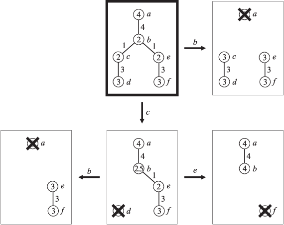
The original network is a $p$ -core at level 2. Applying the algorithm to the network we have three choices for the first vertex to be deleted: $b$ , $c$ or $e$ . Deleting $b$ we get, after removing the isolated vertex $a$ , the $p$ -core $C_{1}=\{c,d,e,f\}$ at level 3. Note that the values of $p$ in vertices $c$ and $e$ increased from 2 to 3.

Deleting $c$ (or symmetrically $e$ – we analyze only the first case) we get the set $C_{2}=\{a,b,e,f\}$ at level 2 – the value at $b$ increased to 2.5. In the next step we can delete either the vertex $b$ , producing the set $C_{3}=\{e,f\}$ at level 3, or the vertex $e$ , producing the $p$ -core $C_{4}=\{a,b\}$ at level 4.

As we see, the result of the algorithm depends on the order of deletions. The $p$ -core at level 4 is not contained in the $p$ -core at level 3.

3 Algorithms

3.1 Algorithm for $p$ -core at level $t$

The $p$ function is local iff

p(v,U)=p(v,N(v,U))

The functions $p_{1}$ – $p_{6}$ from examples are local; $p_{7}$ is not local for $k\geq 4$ .

In the following we shall assume also that for the function $p$ there exists a constant $p_{0}$ such that

\forall v\in V:p(v,\emptyset)=p_{0}

For a local $p$ function an $O(m\max(\Delta,\log n))$ algorithm for determining $p$ -core at level $t$ exists (assuming that $p(v,N(v,C))$ can be computed in $O(\deg_{C}(v))$ ).

INPUT: graph $G=(V,L)$ represented by lists of neighbors and $t\in\hbox{\sf I\kern-1.4pt\hbox{R}}$
OUTPUT: $C\subseteq V$ , $C$ is a $p$ -core at level $t$

1.	$C:=V$ ;
2.	for $v\in V$ do $p[v]:=p(v,N(v,C))$ ;
3.	$build\_min\_heap(v,p)$ ;
4.	while $p[top]<t$ do begin
4.1.		$C:=C\setminus\{top\}$ ;
4.2.		for $v\in N(top,C)$ do begin
4.2.1.			$p[v]:=p(v,N(v,C))$ ;
4.2.2.			$update\_heap(v,p)$ ;
		end;
	end;

The step 4.2.1. can often be speeded up by updating the $p[v]$ .

This algorithm is straightforwardly extended to produce the hierarchy of $p$ -cores. The hierarchy is determined by the core-number assigned to each vertex – the highest level value of $p$ -cores that contain the vertex.

3.2 Determining the hierarchy of $p$ -cores

INPUT: graph $G=(V,L)$ represented by lists of neighbors
OUTPUT: table $core$ with core number for each vertex

1.	$C:=V$ ;
2.	for $v\in V$ do $p[v]:=p(v,N(v,C))$ ;
3.	$build\_min\_heap(v,p)$ ;
4.	while $sizeof(heap)>0$ do begin
4.1.		$C:=C\setminus\{top\}$ ;
4.2.		$core[top]:=p[top]$ ;
4.3.		for $v\in N(top,C)$ do begin
4.3.1.			$p[v]:=\max{\{p[top],p(v,N(v,C))\}}$ ;
4.3.2.			$update\_heap(v,p)$ ;
		end;
	end;

Let us assume that $P$ is a maximum time needed for computing the value of $p(v,U)$ , $v\in V$ , $U\subseteq V$ . Then the complexity of statements 1. – 3. is $T_{1-3}=O(n)+O(Pn)+O(n\log n)=O(n\cdot\max(P,\log n))$ . Let us now look at the body of the while loop. Since at each repetition of the body the size of the set $C$ is decreased by 1 there are at most $n$ repetitions. Statements 4.1 and 4.2 can be implemented to run in constant time, thus contributing $T_{4.1,4.2}=O(n)$ to the loop. In all combined repetitions of the while and for loops each line is considered at most once. Therefore the body of the for loop (statements 4.3,1 and 4.3.2) is executed at most $m$ times – contributing at most $T_{4.3}=m\cdot(P+O(\log n))$ to the while loop. Often the value $p(v,N(v,C))$ can be updated in constant time – $P=O(1)$ . Summing up all the contributions we get the total time complexity of the algorithm $T=T_{1-3}+T_{4.1,4.2}+T_{4.3}=O(m\cdot\max(P,\log n))$ .

For a local $p$ function, for which the value of $p(v,N(v,C))$ can be computed in $O(\deg_{C}(v))$ ), we have $P=O(\Delta)$ .

The described algorithm is partially implemented in program for large networks analysis Pajek (Slovene word for Spider) for Windows (32 bit) [1]. It is freely available, for noncommercial use, at its homepage:

http://vlado.fmf.uni-lj.si/pub/networks/pajek/
A standalone implementation of the algorithm in C is available at

http://www.educa.fmf.uni-lj.si/datana/pub/networks/cores/
For the property functions $p_{1}$ – $p_{4}$ a quicker $O(m)$ core determining algorithm can be developed [4].

4 Example – Internet Connections

Table 1:

p_{5}

-cores of the Routing Data Network at Different Levels.

$k$	$t$	$n$	$k$	$t$	$n$
1	1	7582	12	2048	490
2	2	9288	13	4096	314
3	4	12519	14	8192	153
4	8	33866	15	16384	48
5	16	33757	16	32768	44
6	32	11433	17	65536	11
7	64	6518	18	131072	9
8	128	3812	19	262144	0
9	256	2356	20	524288	2
10	512	1528	21	1048576	3
11	1024	918

As an example of application of the proposed algorithm we applied it to the routing data on the Internet network. This network was produced from web scanning data (May 1999) available from

http://www.cs.bell-labs.com/who/ches/map/index.html
It can be obtained also as a Pajek’s NET file from

http://vlado.fmf.uni-lj.si/pub/networks/data/web/web.zip
It has $124\ 651$ vertices, $195\ 029$ arcs (loops were removed), $\Delta=151$ , and average degree is $3.13$ . The arcs have as values the number of traceroute paths which contain the arc.

Using Pajek implementation of the proposed algorithm on 300 MHz PC we obtained in 3 seconds the $p_{5}$ -cores segmentation presented in Table 1 – there are $n_{k}$ vertices with $p_{5}$ -core number in the interval $(t_{k-1},t_{k}]$ .

The program also determined the $p_{5}$ -core number for every vertex. Figure 3 shows a $p_{5}$ -core at level 25000 of the Internet network – every vertex inside this core is visited by at least 25000 traceroute paths. In the figure the sizes of circles representing vertices are proportional to (the square roots of) their $p_{5}$ -core numbers. Since the arcs values span from 1 to 626826 they can not be displayed directly. We recoded them according to the thresholds $1000\cdot 2^{k-1}$ , $k=1,2,3\ldots$ . These class numbers are represented by the thickness of the arcs.

5 Conclusions

The cores, because they can be efficiently determined, are one among few concepts that provide us with meaningful decompositions of large networks [5]. We expect that different approaches to the analysis of large networks can be built on this basis. For example, the sequence of vertices in sequential coloring can be determined by descending order of their core numbers (combined with their degrees). We obtain in this basis the following bound on the chromatic number of a given graph $\mathbf{G}$

\chi(\mathbf{G})\leq 1+\mbox{\rm core}(\mathbf{G})

Cores can also be used to localize the search for interesting subnetworks in large networks [3, 2]:

•

If it exists, a $k$ -component is contained in a $k$ -core.
•

If it exists, a $k$ -clique is contained in a $k$ -core. $\omega(\mathbf{G})\leq\mbox{\rm core}(\mathbf{G})$ .

References

Batagelj and Mrvar (1998) Batagelj, V. and Mrvar, A. 1998. Pajek – a program for large network analysis. Connections 21 (2), 47–57.
Batagelj and Mrvar (2000) Batagelj, V. and Mrvar, A. 2000. Some analyses of Erdős collaboration graph. Social Networks 22, 173–186.
Batagelj et al. (1999) Batagelj, V., Mrvar, A., and Zaveršnik, M. 1999. Partitioning approach to visualization of large graphs. In Graph drawing, J. Kratochvíl, Ed. Lecture notes in computer science, 1731. Springer, Berlin, 90–97.
Batagelj and Zaveršnik (2001) Batagelj, V. and Zaveršnik, M. 2001. An $O(m)$ algorithm for cores decomposition of networks. Manuscript, Submitted.
Garey and Johnson (1979) Garey, M. R. and Johnson, D. S. 1979. Computer and intractability. Freeman, San Francisco.
Seidman (1983) Seidman, S. B. 1983. Network structure and minimum degree. Social Networks 5, 269–287.
Wasserman and Faust (1994) Wasserman, S. and Faust, K. 1994. Social network analysis: Methods and applications. Cambridge University Press, Cambridge.

eceived Month Year; revised Month Year; accepted Month Year

Generalized Cores

Abstract

Keywords:

category

keywords

keywords

1 Cores

2 pp-cores

Theorem 2.1

Proof.

Corollary 2.2

Proof.

3 Algorithms

3.1 Algorithm for pp-core at level tt

3.2 Determining the hierarchy of pp-cores

4 Example – Internet Connections

5 Conclusions

References

2 $p$ -cores

3.1 Algorithm for $p$ -core at level $t$

3.2 Determining the hierarchy of $p$ -cores