Optimization Over Zonotopes and
Training Support Vector Machines
Abstract
We make a connection between classical polytopes called zonotopes and Support Vector Machine (SVM) classifiers. We combine this connection with the ellipsoid method to give some new theoretical results on training SVMs. We also describe some special properties of -SVMs for .
1 Introduction
A statistical classifier algorithm maps a set of training vectors—positively and negatively labeled points in —to a decision boundary. A Support Vector Machine (SVM) is a classifier algorithm in which the decision boundary depends on only a subset of training vectors, called the support vectors [18]. This limited dependence on the training set helps give SVMs good generalizability, meaning that SVMs are resistant to overtraining even in the case of large . Another key idea associated with SVMs is the use of a kernel function in computing the dot product of two training vectors. For example, the usual dot product could be replaced by (quadratic kernel) or by (radial basis function). The kernel function [14] in effect maps the original training vectors in into a higher-dimensional (perhaps infinite-dimensional) feature space ; a linear decision boundary in then determines a nonlinear decision surface back in . For good introductions to SVMs see the tutorial by Burges [3] or the book by Cristianini and Shawe-Taylor [6].
The basic maximum margin SVM applies to the case of linearly separable training vectors, and divides positive and negative vectors by a farthest-apart pair of parallel hyperplanes, as shown in Figure 1(a). The decision boundary itself is typically the hyperplane halfway between the boundaries. Computational geometers might expect that the extension of the SVM to the non-separable case would divide positive and negative vectors by a least-overlapping pair of half-spaces bounded by parallel hyperplanes, as shown in Figure 1(b). This generalization, however, may be overly sensitive to outliers, and hence the method of choice is a more robust soft margin classifier, called a -SVM [4, 18] or -SVM [13] depending upon the precise formulation. Parameter is a user-chosen penalty for errors.
Computing the maximum margin classifier for vectors in amounts to solving a quadratic program (QP) with about variables and linear constraints. If the feature vectors are not explicit (that is, kernel functions are being used), then the usual Lagrangian formulation gives a QP with about variables and linear constraints. Similarly, the soft margin classifier—with or without explicit feature vectors—is computed in a Lagrangian formulation with about variables and linear constraints. The jump from to variables can have a great impact on the running time and choice of QP algorithm. Recent results in computational geometry [8, 11] give fast QP algorithms for the case of large and small , algorithms requiring about arithmetic operations. The best bound on the number of arithmetic operations for a QP with variables and constraints is about , where is the precision of the input data [16].
In this paper, we show that the jump from to is not necessary for soft margin classifiers with explicit feature vectors. More specifically, we describe training algorithms with running time near linear in and polynomial in and input precision, for two different scenarios: set by the user and . The second scenario also introduces a natural measure of separability of point sets. Our algorithms build upon a geometric view of soft margin classifiers [1, 5] and the ellipsoid method for convex optimization. Due to their reliance on explicit feature vectors and the ellipsoid method, and also due to the fact that SVMs are more suited to the case of moderate and large than to the case of large and small , our algorithms have little practical importance. On the other hand, our results should be interesting theoretically. We view the soft margin classifier as a problem defined over a zonotope, a type of polytope that admits an especially compact description. Accordingly, our algorithms have lower complexity than either the vertex or facet descriptions of the polytopes.

2 SVM Formulations
We adopt the usual SVM notation and mostly follow the presentation of Bennett and Bredensteiner [1]. The training vectors are , points in . The corresponding labels are , each of which is either or . Let and . We use and to denote vectors in and to denote a scalar. We use the dot product notation , but in this section could be standing in for the kernel function .
In the maximum margin SVM we seek parallel hyperplanes defined by the equations and such that for all and for all . The signed distance between these two hyperplanes—the margin—is and hence can be maximized by minimizing .
| (1) | |||||
A popular choice for the decision boundary is the plane halfway between the parallel hyperplanes, , and hence each unknown vector is classified according to the sign of .
In the linearly separable case, we can set and (thereby rescaling ) and obtain the following optimization problem, the standard form in most SVM treatments [3].
| (2) | |||||
Notice that this QP has variables and linear constraints. At the solution, is a linear combination of ’s, gives the margin, and gives the halfway decision boundary.
The dual problem to maximizing the distance between parallel hyperplanes separating the positive and negative convex hulls is to minimize the distance between points inside the convex hulls. Thus the dual in the separable case is the following.
| (3) |
Karush-Kuhn-Tucker (complementary slackness) conditions show that the optimizing value of for (1) is given by the optimizing values of for (3): . The vectors with are called the support vectors.
The soft margin SVM adds slack variables to formulation (1), and then penalizes solutions proportional to the sum of these variables. Slack variable measures the error for training vector , that is, how far lies on the wrong side of the parallel hyperplane for ’s class.
| (4) | |||||
The standard -SVM formulation [18] again sets and .
| (5) | |||||
In formulation 5, the decision boundary is . Formulation (4), however, does not set the decision boundary, but only its direction. Crisp and Burges [5] write that because “originally the sum of ’s term arose in an attempt to approximate the number of errors”, the best option might be to run a “simple line search” to find the decision boundary that actually minimizes the number of training set errors.
The dual of formulation (4) in the separable case minimizes the distance between points inside “reduced” or “soft” convex hulls [1, 5].
| (6) |
See Figure 2. The reduced convex hull of points , , is the set of convex combinations of with each . (Notice that in (4) there is no reason to consider .) We shall say more about reduced convex hulls in the next section.

The dual view highlights a slight difference between formulations (4) and (5). Formulation (4) allows the direct setting of the reduced convex hulls. Parameter limits the influence of any single training point; if the user expects no more than four outliers in the training set, then an appropriate choice of might be in order to ensure that the majority of the support vectors are non-outliers. If the reduced convex hulls intersect, the solution to (4) is the least-overlapping pair of half-spaces, as in Figure 1(b). Formulation (5) is also always feasible—unlike the standard hard margin formulation (2)—but it never allows the reduced convex hulls to intersect. As the reduced convex hulls either fill out their convex hulls (the separable case) or continue growing until they asymptotically touch (the non-separable case).
3 Reduced Convex Hulls and Zonotopes
Assume and define the positive and negative reduced convex hulls by
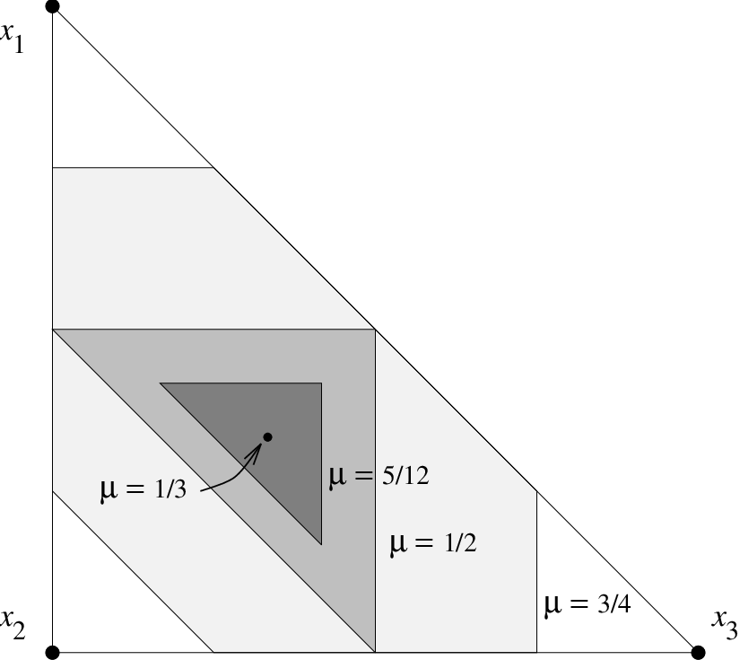
Figure 3 shows the reduced convex hull of three points , , and for various values of . The reduced convex hull grows from the centroid at to the convex hull at ; for it is empty. In Figure 2, is a little less than .
A reduced convex hull is a special case of a centroid polytope, the locus of possible weighted averages of points each with an unknown weight within a certain range [2]. For reduced convex hulls, each weight has the same range and the sum of the weights is constrained to be . In [2] we related centroid polytopes in to special polytopes, called zonotopes, in . We repeat the connection here, specialized to the case of reduced convex hulls.
Let denote , the vector in that agrees with on its first coordinates and has 1 as its last coordinate. Define
Polytope is a Minkowski sum11 1 The Minkowski sum of sets and in is . of line segments of the form . The Minkowski sum of line segments is a special type of convex polytope called a zonotope [2, 7]. Polytope is the cross-section of with the -st coordinate (which by construction is also ) equal to one. Of course, can also be related to a zonotope in the same way. The following lemmas state the property of zonotopes and reduced convex hulls that underlies our algorithms. Lemma 2 is implicit in Keerthi et al.’s iterative nearest-point approach to SVM training [9].
Lemma 1
Let be a zonotope that is the Minkowski sum of line segments in . There is an algorithm with arithmetic operations for optimizing a linear function over .
Proof
Assume that we are trying to find a vertex in zonotope extreme in direction , that is, that maximizes the dot product . Assume that is the Minkowski sum of line segments of the form , where . We simply set each independently to or , depending upon whether the projection of onto is negative or positive.
Lemma 2
There is an algorithm with arithmetic operations for optimizing a linear function over a reduced convex hull of points in .
Proof
Assume that we are trying to find a vertex in zonotope extreme in direction . Order the ’s with according to their projection onto vector , breaking ties arbitrarily. In decreasing order by projection along , set the corresponding ’s to until doing so would violate the constraint that . Set for this “transitional” vector to the maximum value allowed by this constraint, and finally set the remaining ’s to . Then maximizes .
An interesting combinatorial question asks for the worst-case complexity of a reduced convex hull . The vertex of that is extreme for direction can be associated with the set of ’s for which . If , then as in Lemma 2, ’s set is the first points in direction , a set of points that can be separated from the other points by a hyperplane normal to . And conversely, each separable set of points defines a unique vertex of . Hence the maximum number of vertices of is equal to the maximum number of -sets for points in , which is known to be and [17, 19]. In [2] we showed that a more general centroid polytope in which each point has between and (that is, different weight bounds for different points) may have complexity .
We can also apply the argument in the proof of Lemma 2 to say something about the optimizing values of the variables in (4) and (6) for the non-separable case. (Alternatively we can derive the same statements from the Karush-Kuhn-Tucker conditions.) Each of and has a transition in the sorted order of the ’s when projected along the normal to the parallel pair of hyperplanes. For with , if lies on the “right” side of the transition, if coincides with the transition, and if lies on the “wrong” side of the transition. Of course an analogous statement holds for for . As usual, the support vectors are those with . Thus all training set errors are support vectors. In Figure 2(a) there are six support vectors: two transitional unfilled dots (marked and ) and one wrong-side unfilled dot, along with one transitional and two wrong-side filled dots.
4 Ellipsoid-Based Algorithms
We first assume that has been fixed in advance, perhaps using some knowledge of the expected number of outliers or the desired number of support vectors. We give an algorithm for solving formulation (6).
One approach would be to compute the vertices of and and then use formulation (1) with positive and negative training vectors replaced by the vertices of and respectively. However, the number of vertices of and may be very large, so this algorithm could be very slow.
So instead we exploit a polynomial-time equivalence between separation and optimization (see for example [15], chapter 14.2). The input to the separation problem is a point and a polytope (typically given by a system of linear inequalities). The output is either a statement that is inside or a hyperplane separating and . The input to the optimization problem is a direction and a polytope . The output is either a statement that is empty, a statement that is unbounded in direction , or a point in extreme for direction . The two problems are related by projective duality,22 2 The more famous direction of this equivalence is that separation—which can be solved directly by checking each inequality—implies optimization. This result is a corollary of Khachiyan’s ellipsoid method. and a subroutine for solving one can be used to solve the other in a number of calls that is polynomial in the dimension and the input precision, that is, the number of bits in or plus the maximum number of bits in an inequality defining .
In our case, the polytope is not given by inequalities, but rather as a Minkowski sum of line segments; this presentation has an impact on the required precision. If the input precision is , the maximum number of bits in one of the feature vectors , then the maximum number of bits in a vertex of the polytope is . What is new is the term, resulting from the fact that a vertex of a zonotope is a sum of up to input vectors.
Theorem 4.1
Given explicit feature vectors in and with , there is a polynomial-time algorithm for computing a soft margin classifier, with the number of arithmetic operations linear in and polynomial in , , and .
Proof
As in [9], consider the polytope that is the Minkowski sum of and , that is, . We are trying to minimize over the convex quadratic objective function , that is, the length of a line segment between and .
For a given direction , we can find the solution to the linear optimization problem for by using Lemma 2 to find the optimizing over and the optimizing over . Now given a point , we can use this observation and the polynomial-time equivalence between separation and optimization to solve the separation problem for and in time linear in and polynomial in and . We can use this solution to the separation problem for as a subroutine for the ellipsoid method (see [10, 15]) in order to optimize over . Given an optimizing choice of , it is easy to find the best pair of parallel hyperplanes and a decision boundary, either the -SVM decision boundary or some other reasonable choice within the parallel family.
Now assume that we are in the non-separable case. We shall show how to solve for the maximum for which the reduced convex hulls have non-intersecting interior, that is, the for which the margin is . This choice of corresponds to and the objective function simplifying to in formulation (5).
This choice of has two special properties. First, among all settings of , tends to give the fewest support vectors. To see this, imagine shrinking the shaded regions in Figure 2(a). Support vectors are added each time one of the parallel hyperplanes crosses a training vector. On the other hand, a support vector may be lost occasionally when the number of reduced convex hull vertices on the parallel hyperplanes changes, for example, if the vertex supporting the upper parallel line in Figure 2(a) slipped off to the right of the segment supporting the lower parallel line.
Second, the for which the margin is zero gives a natural measure of the separability of two point sets. For simplicity, let and normalize the zero-margin by . The separability measure runs from 0 to 1, with 0 meaning that the centroids coincide and 1 meaning that the convex hulls have disjoint interiors. Computing the zero-margin as the maximum value of a dual variable using formulation (5) above is no harder than training a -SVM, and in the case of explicit features, it should be significantly easier, as we now show.
We can formulate the problem as minimizing subject to
As above, let denote , the vector in that agrees with on its first coordinates and has 1 as its last coordinate. Letting , we can rewrite the problem as maximizing
subject to
| (7) |
Yet another way to state the problem is to ask for the point with maximum -st coordinate in , where
Polytopes and are each zonotopes, Minkowski sums of line segments of the form .
Theorem 4.2
Let and be zonotopes defined by a total of line segments in . There is an algorithm for optimizing a linear objective function over , with the number of arithmetic operations linear in and polynomial in , , and .
Proof
Given a point and zonotope , , we can use Lemma 1 and the polynomial-time equivalence between separation and optimization to solve the separation problem for and in time linear in and polynomial in , and . We can solve the separation problem for the intersection of zonotopes simply by solving it separately for each zonotope. We now use the equivalence between separation and optimization in the other direction to conclude that we can also solve the optimization problem for an intersection of zonotopes.
The proof of the following result then follows from the ellipsoid method in the same way as the proof of Theorem 4.1.
Corollary 1
Given explicit feature vectors in , there is a polynomial-time algorithm for computing the maximum for which and are linearly separable, with the number of arithmetic operations linear in and polynomial in , , and .
Theorem 4.1 and Corollary 1 can be extended to some cases of implicit feature vectors. For example, the quadratic kernel for vectors and in is equivalent to an ordinary dot product in , namely , where . In general [3], a polynomial kernel amounts to lifting the training vectors from to where . Radial basis functions, however, give , and the SVM training problem seems to necessarily involve variables. (The rather amazing part is that it is a combinatorial optimization problem at all!)
5 Discussion and Conclusions
In this paper we have connected SVMs to some recent results in computational geometry and mathematical programming. These connections raise some new questions, both practical and theoretical.
Currently the best practical algorithms for training SVMs, Platt’s sequential minimal optimization (SMO) [12] and Keerthi et al.’s nearest point algorithm (NPA) [9], can be viewed as interior-point methods that iteratively optimize the margin over line segments. Both algorithms make use of heuristics to find line segments close to the exterior, meaning line segments with weights set to either 0 or .
Computational geometry may have a practical algorithm to contribute for the case of large and small, say and : the generalized linear programming (GLP) paradigm of Matoušek et al. [8, 11]. The training vectors need not actually live in for small , so long as the GLP dimension of the problem is small, where the GLP dimension is the number of support vectors in any subproblem defined by a subset of the training vectors.
On the theoretical side, we are wondering about the existence of strongly polynomial algorithms for QP problems over zonotopes. Due to the combinatorial equivalence of zonotopes and arrangements, the graph diameter of a zonotope is known to be only ; polynomial graph diameter is of course a necessary condition for the existence of a polynomial-time simplex-style algorithm.
Acknowledgments
David Eppstein’s work was done in part while visiting Xerox PARC, and supported in part by NSF grant CCR-9912338. We would also like to thank Yoram Gat for a number of helpful discussions.
References
- [1] K.P. Bennett and E.J. Bredensteiner. Duality and geometry in SVM classifiers. Proc. 17th Int. Conf. Machine Learning, Pat Langley, ed., Morgan Kaufmann, 2000, 57–64.
- [2] M. Bern, D. Eppstein, L. Guibas, J. Hershberger, S. Suri, and J. Wolter. The centroid of points with approximate weights. 3rd European Symposium on Algorithms, Corfu, 1995. Springer Verlag LNCS 979, 1995, 460–472.
- [3] C.J.C. Burges. A tutorial on support vector machines for pattern recognition. Data Mining and Knowledge Discovery, Vol. 2, No. 2, 1998, 121–167. http://svm.research.bell-labs.com/SVMrefs.html
- [4] C. Cortes and V. Vapnik. Support vector networks. Machine Learning, 1995, 273–297.
- [5] D.J. Crisp and C.J.C. Burges. A geometric interpretation of -SVM classifiers. Advances in Neural Information Processing Systems 12. S.A. Solla, T.K. Leen, and K.-R. Müller, eds. MIT Press, 1999. http://svm.research.bell-labs.com/SVMrefs.html
- [6] N. Cristianini and J. Shawe-Taylor. Support Vector Machines. Cambridge U. Press, 2000.
- [7] H. Edelsbrunner. Algorithms in Combinatorial Geometry, Springer Verlag, 1987.
- [8] B. Gärtner. A subexponential algorithm for abstract optimization problems. SIAM J. Computing 24 (1995), 1018–1035.
- [9] S.S. Keerthi, S.K. Shevade, C. Bhattacharyya, and K.R.K. Murthy. A fast iterative nearest point algorithm for support vector machine classifier design. IEEE Trans. Neural Networks 11 (2000), 124–136. http://guppy.mpe.nus.edu.sg/~mpessk/
- [10] M.K. Kozlov, S.P. Tarasov, L.G. Khachiyan. Polynomial solvability of convex quadratic programming. Soviet Math. Doklady 20 (1979) 1108–1111.
- [11] J. Matoušek, M. Sharir, and E. Welzl. A subexponential bound for linear programming. Tech. Report B 92-17, Freie Univ. Berlin, Fachb. Mathematik, 1992
- [12] J.C. Platt. Fast training of support vector machines using sequential minimal optimization. Chapter 12 of Advances in Kernel Methods: Support Vector Learning, B. Schölkopf, C. Burges, and A. Smola, eds. MIT Press, 1998, 185–208. http://www.research.microsoft.com/~jplatt
- [13] B. Schölkopf, A.J. Smola, R. Williamson, and P. Bartlett. New support vector algorithms. Neural Computatation Vol. 12, No. 5, 2000, 1207–1245. NeuroCOLT2 Technical Report NC2-TR-1998-031. 1998. http://svm.first.gmd.de/papers/tr-31-1998.ps.gz
- [14] B. Schölkopf, S. Mika, C.J.C. Burges, P. Knirsch, K.-R. Müller, G. Rätsch, and A.J. Smola. Input space vs. feature space in kernel-based methods. IEEE Trans. on Neural Networks 10 (1999) 1000-1017. http://svm.research.bell-labs.com/SVMrefs.html
- [15] A. Schrijver. Theory of Linear and Integer Programming John Wiley & Sons, 1986.
- [16] M.J. Todd. Mathematical Programming. Chapter 39 of Handbook of Discrete and Computational Geometry, J.E. Goodman and J. O’Rourke, eds., CRC Press, 1997.
- [17] G. Tóth. Point sets with many -sets. Proc. 16th Annual ACM Symp. Computational Geometry, 2000, 37–42.
- [18] V. Vapnik. Statistical Learning Theory. Wiley, 1998.
- [19] R.T. Živaljević and S.T. Vrećica. The colored Tverberg’s problem and complexes of injective functions. J. Comb. Theory, Series A, 61 (1992) 309–318.