Robust Classification for Imprecise Environments
Foster Provost provost@acm.org
New York University, New York, NY 10012
Tom Fawcett tfawcett@acm.org
Hewlett-Packard Laboratories, Palo Alto, CA 94304
Keywords: classification, learning, uncertainty, evaluation, comparison, multiple models, cost-sensitive learning, skewed distributions
To appear in Machine Learning Journal
Abstract
In real-world environments it usually is difficult to specify target operating conditions precisely, for example, target misclassification costs. This uncertainty makes building robust classification systems problematic. We show that it is possible to build a hybrid classifier that will perform at least as well as the best available classifier for any target conditions. In some cases, the performance of the hybrid actually can surpass that of the best known classifier. This robust performance extends across a wide variety of comparison frameworks, including the optimization of metrics such as accuracy, expected cost, lift, precision, recall, and workforce utilization. The hybrid also is efficient to build, to store, and to update. The hybrid is based on a method for the comparison of classifier performance that is robust to imprecise class distributions and misclassification costs. The ROC convex hull (rocch) method combines techniques from ROC analysis, decision analysis and computational geometry, and adapts them to the particulars of analyzing learned classifiers. The method is efficient and incremental, minimizes the management of classifier performance data, and allows for clear visual comparisons and sensitivity analyses. Finally, we point to empirical evidence that a robust hybrid classifier indeed is needed for many real-world problems.
1 Introduction
Traditionally, classification systems have been built by experimenting with many different classifiers, comparing their performance and choosing the best. Experimenting with different induction algorithms, parameter settings, and training regimes yields a large number of classifiers to be evaluated and compared. Unfortunately, comparison often is difficult in real-world environments because key parameters of the target environment are not known. The optimal cost/benefit tradeoffs and the target class priors seldom are known precisely, and often are subject to change [\BCAYZahavi \BBA LevinZahavi \BBA Levin1997, \BCAYFriedman \BBA WyattFriedman \BBA Wyatt1997, \BCAYKlinkenberg \BBA ThorstenKlinkenberg \BBA Thorsten2000]. For example, in fraud detection we cannot ignore misclassification costs or the skewed class distribution, nor can we assume that our estimates are precise or static [\BCAYFawcett \BBA ProvostFawcett \BBA Provost1997]. We need a method for the management, comparison, and application of multiple classifiers that is robust in imprecise and changing environments.
We describe the ROC convex hull (rocch) method, which combines techniques from ROC analysis, decision analysis and computational geometry. The ROC convex hull decouples classifier performance from specific class and cost distributions, and may be used to specify the subset of methods that are potentially optimal under any combination of cost assumptions and class distribution assumptions. The rocch method is efficient, so it facilitates the comparison of a large number of classifiers. It minimizes the management of classifier performance data because it can specify exactly those classifiers that are potentially optimal, and it is incremental, easily incorporating new and varied classifiers without having to reevaluate all prior classifiers.
We demonstrate that it is possible and desirable to avoid complete commitment to a single best classifier during system construction. Instead, the rocch can be used to build from the available classifiers a hybrid classification system that will perform best under any target cost/benefit and class distributions. Target conditions can then be specified at run time. Moreover, in cases where precise information is still unavailable when the system is run (or if the conditions change dynamically during operation), the hybrid system can be tuned easily (and optimally) based on feedback from its actual performance.
The paper is structured as follows. First we sketch briefly the traditional approach to building such systems, in order to demonstrate that it is brittle under the types of imprecision common in real-world problems. We then introduce and describe the rocch and its properties for comparing and visualizing classifier performance in imprecise environments. In the following sections we formalize the notion of a robust classification system, and show that the rocch is an elegant method for constructing one automatically. The solution is elegant because the resulting hybrid classifier is robust for a wide variety of problem formulations, including the optimization of metrics such as accuracy, expected cost, lift, precision, recall, and workforce utilization, and it is efficient to build, to store, and to update. We then show that the hybrid actually can do better than the best known classifier in certain situations. Finally, by citing results from empirical studies, we provide evidence that this type of system indeed is needed.
1.1 An example
A systems-building team wants to create a system that will take a large number of instances and identify those for which an action should be taken. The instances could be potential cases of fraudulent account behavior, of faulty equipment, of responsive customers, of interesting science, etc. We consider problems for which the best method for classifying or ranking instances is not well defined, so the system builders may consider machine learning methods, neural networks, case-based systems, and hand-crafted knowledge bases as potential classification models. Ignoring for the moment issues of efficiency, the foremost question facing the system builders is: which of the available models performs “best” at classification?
Traditionally, an experimental approach has been taken to answer this question, because the distribution of instances can be sampled if it is not known a priori. The standard approach is to estimate the error rate of each model statistically and then to choose the model with the lowest error rate. This strategy is common in machine learning, pattern recognition, data mining, expert systems and medical diagnosis. In some cases, other measures such as cost or benefit are used as well. Applied statistics provides methods such as cross-validation and the bootstrap for estimating model error rates and recent studies have compared the effectiveness of different methods [\BCAYDietterichDietterich1998, \BCAYKohaviKohavi1995, \BCAYSalzbergSalzberg1997].
Unfortunately, this experimental approach is brittle under two types of imprecision that are common in real-world environments. Specifically, costs and benefits usually are not known precisely, and target (prior) class distributions often are known only approximately as well. This observation has been made by many authors [\BCAYBradleyBradley1997, \BCAYCatlettCatlett1995, \BCAYProvost \BBA FawcettProvost \BBA Fawcett1997], and is in fact the concern of a large subfield of decision analysis [\BCAYWeinstein \BBA FinebergWeinstein \BBA Fineberg1980]. Imprecision also arises because the environment may change between the time the system is conceived and the time it is used, and even as it is used. For example, levels of fraud and levels of customer responsiveness change continually over time and from place to place.
1.2 Basic terminology

In this paper we address two-class problems. Formally, each instance is mapped to one element of the set of (correct) positive and negative classes. A classification model (or classifier) is a mapping from instances to predicted classes. Some classification models produce a continuous output (e.g., an estimate of an instance’s class membership probability) to which different thresholds may be applied to predict class membership. To distinguish between the actual class and the predicted class of an instance, we will use the labels for the classifications produced by a model. For our discussion, let be a two-place error cost function where is the cost of a false positive error and is the cost of a false negative error.11 1 For this paper, we consider error costs to include benefits not realized, and ignore the costs of correct classifications. We represent class distributions by the classes’ prior probabilities and .
The true positive rate, or hit rate, of a classifier is:
The false positive rate, or false alarm rate, of a classifier is:
The traditional experimental approach is brittle because it chooses one model as “best” with respect to a specific set of cost functions and class distribution. If the target conditions change, this system may no longer perform optimally, or even acceptably. As an example, assume that we have a maximum false positive rate , that must not be exceeded. We want to find the classifier with the highest possible true positive rate, , that does not exceed the limit. This is the Neyman-Pearson decision criterion [\BCAYEganEgan1975]. Three classifiers, under three such limits, are shown in figure 1. A different classifier is best for each limit; any system built with a single “best” classifier is brittle if the requirement can change.
2 Evaluating and visualizing classifier performance
2.1 Classifier comparison: decision analysis and ROC analysis
Most prior work on building classifiers uses classification accuracy (or, equivalently, undifferentiated error rate) as the primary evaluation metric. The use of accuracy assumes that the class priors in the target environment will be constant and relatively balanced. In the real world this rarely is the case. Classifiers often are used to sift through a large population of normal or uninteresting entities in order to find a relatively small number of unusual ones; for example, looking for defrauded accounts among a large population of customers, screening medical tests for rare diseases, and checking an assembly line for defective parts. Because the unusual or interesting class is rare among the general population, the class distribution is very skewed [\BCAYEzawa, Singh, \BBA NortonEzawa et al.1996, \BCAYFawcett \BBA ProvostFawcett \BBA Provost1996, \BCAYFawcett \BBA ProvostFawcett \BBA Provost1997, \BCAYKubat, Holte, \BBA MatwinKubat et al.1998, \BCAYSaitta \BBA NeriSaitta \BBA Neri1998].
As the class distribution becomes more skewed, evaluation based on accuracy breaks down. Consider a domain where the classes appear in a 999:1 ratio. A simple rule—always classify as the maximum likelihood class—gives a 99.9% accuracy. This accuracy may be quite difficult for an induction algorithm to beat, though the simple rule presumably is unacceptable if a non-trivial solution is sought. Skews of are common in fraud detection and skews exceeding have been reported in other applications [\BCAYClearwater \BBA SternClearwater \BBA Stern1991].
Evaluation by classification accuracy also assumes equal error costs: . In the real world classifications lead to actions, which have consequences. Actions can be as diverse as denying a credit charge, discarding a manufactured part, moving a control surface on an airplane, or informing a patient of a cancer diagnosis. The consequences may be grave, and performing an incorrect action may be very costly. Rarely are the costs of mistakes equivalent. In mushroom classification, for example, judging a poisonous mushroom to be edible is far worse than judging an edible mushroom to be poisonous. Indeed, it is hard to imagine a domain in which a classification system may be indifferent to whether it makes a false positive or a false negative error. In such cases, accuracy maximization should be replaced with cost minimization.
The problems of unequal error costs and uneven class distributions are related. It has been suggested that, for training, high-cost instances can be compensated for by increasing their prevalence in an instance set [\BCAYBreiman, Friedman, Olshen, \BBA StoneBreiman et al.1984]. Unfortunately, little work has been published on either problem. There exist several dozen articles in which techniques for cost-sensitive learning are suggested [\BCAYTurneyTurney1996], but few studies evaluate and compare them [\BCAYDomingosDomingos1999, \BCAYPazzani, Merz, Murphy, Ali, Hume, \BBA BrunkPazzani et al.1994, \BCAYProvost, Fawcett, \BBA KohaviProvost et al.1998]. The literature provides even less guidance in situations where distributions are imprecise or can change.

Given an estimate of , the posterior probability of an instance’s class membership, decision analysis gives us a way to produce cost-sensitive classifications [\BCAYWeinstein \BBA FinebergWeinstein \BBA Fineberg1980]. Classifier error frequencies can be used to approximate such probabilities [\BCAYPazzani, Merz, Murphy, Ali, Hume, \BBA BrunkPazzani et al.1994]. For an instance , the decision to emit a positive classification from a particular classifier is:
Regardless of whether a classifier produces probabilistic or binary classifications, its normalized cost on a test set can be evaluated empirically as:
Most published work on cost-sensitive classification uses an equation such as this to rank classifiers. Given a set of classifiers, a set of examples, and a precise cost function, each classifier’s cost is computed and the minimum-cost classifier is chosen. However, as discussed above, such analyses assume that the distributions are precisely known and static.
More general comparisons can be made with Receiver Operating Characteristic (ROC) analysis, a classic methodology from signal detection theory that is common in medical diagnosis and has recently begun to be used more generally in AI classifier work [\BCAYBeck \BBA SchultzBeck \BBA Schultz1986, \BCAYEganEgan1975, \BCAYSwetsSwets1988, \BCAYFriedman \BBA WyattFriedman \BBA Wyatt1997]. ROC graphs depict tradeoffs between hit rate and false alarm rate.
We use the term ROC space to denote the coordinate system used for visualizing classifier performance. In ROC space, is represented on the Y axis and is represented on the X axis. Each classifier is represented by the point in ROC space corresponding to its pair. For models that produce a continuous output, e.g., posterior probabilities, and vary together as a threshold on the output is varied between its extremes (each threshold defines a classifier); the resulting curve is called the ROC curve. An ROC curve illustrates the error tradeoffs available with a given model. Figure 2 shows a graph of three typical ROC curves; in fact, these are the complete ROC curves of the classifiers shown in figure 1.
For orientation, several points on an ROC graph should be noted. The lower left point represents the strategy of never alarming, the upper right point represents the strategy of always alarming, the point represents perfect classification, and the line (not shown) represents the strategy of randomly guessing the class. Informally, one point in ROC space is better than another if it is to the northwest ( is higher, is lower, or both). An ROC graph allows an informal visual comparison of a set of classifiers.
ROC graphs illustrate the behavior of a classifier without regard to class distribution or error cost, and so they decouple classification performance from these factors. Unfortunately, while an ROC graph is a valuable visualization technique, it does a poor job of aiding the choice of classifiers. Only when one classifier clearly dominates another over the entire performance space can it be declared better.
2.2 The ROC Convex Hull method
In this section we combine decision analysis with ROC analysis and adapt them for comparing the performance of a set of learned classifiers. The method is based on three high-level principles. First, ROC space is used to separate classification performance from class and cost distribution information. Second, decision-analytic information is projected onto the ROC space. Third, the convex hull in ROC space is used to identify the subset of classifiers that are potentially optimal.

2.2.1 Iso-performance lines
By separating classification performance from class and cost distribution assumptions, the decision goal can be projected onto ROC space for a neat visualization. Specifically, the expected cost of applying the classifier represented by a point (,) in ROC space is:
Therefore, two points, (,) and (,), have the same performance if
This equation defines the slope of an iso-performance line. That is, all classifiers corresponding to points on the line have the same expected cost. Each set of class and cost distributions defines a family of iso-performance lines. Lines “more northwest” (having a larger -intercept) are better because they correspond to classifiers with lower expected cost.
2.2.2 The ROC convex hull
Because in most real-world cases the target distributions are not known precisely, it is valuable to be able to identify those classifiers that potentially are optimal. Each possible set of distributions defines a family of iso-performance lines, and for a given family, the optimal methods are those that lie on the “most-northwest” iso-performance line. Thus, a classifier is optimal for some conditions if and only if it lies on the northwest boundary (i.e., above the line ) of the convex hull [\BCAYBarber, Dobkin, \BBA HuhdanpaaBarber et al.1996] of the set of points in ROC space.22 2 The convex hull of a set of points is the smallest convex set that contains the points. We discuss this in detail in Section 3.

We call the convex hull of the set of points in ROC space the ROC convex hull (rocch) of the corresponding set of classifiers. Figure 3 shows four ROC curves with the ROC convex hull drawn as the border between the shaded and unshaded areas. is clearly not optimal. Perhaps surprisingly, can never be optimal either because none of the points of its ROC curve lies on the convex hull. We can also remove from consideration any points of and that do not lie on the hull.
Consider these classifiers under two distribution scenarios. In each, negative examples outnumber positives by 5:1. In scenario , false positive and false negative errors have equal cost. In scenario , a false negative is 25 times as expensive as a false positive (e.g., missing a case of fraud is much worse than a false alarm). Each scenario defines a family of iso-performance lines. The lines corresponding to scenario have slope 5; those for have slope . Figure 4 shows the convex hull and two iso-performance lines, and . Line is the “best” line with slope that intersects the convex hull; line is the best line with slope that intersects the convex hull. Each line identifies the optimal classifier under the given distribution.

Figure 5 shows the three ROC curves from our initial example, with the convex hull drawn.
2.2.3 Generating the ROC Convex Hull
The ROC convex hull method selects the potentially optimal classifiers based on the ROC convex hull and iso-performance lines.
| Given: | E: | List of | tuples where: | |
| : labeled example | ||||
| : numeric ranking assigned to by the classifier | ||||
| : count of positive and negative examples in E, respectively. | ||||
| Output: R: List of points on the ROC curve. | ||||
| ; | /* current TP tally */ | |||
| ; | /* current FP tally */ | |||
| ; | /* last score seen */ | |||
| ; | /* list of ROC points */ | |||
| sort in decreasing order by values; | ||||
| while (E ) do | ||||
| remove tuple from head of E; | ||||
| if () then | ||||
| add point (, ) to end of R; | ||||
| ; | ||||
| end if | ||||
| if ( is a positive example) then | ||||
| ; | ||||
| else | /* I is a negative example */ | |||
| ; | ||||
| end if | ||||
| end while | ||||
| add point (, ) to end of R; |
- 1.
For each classifier, plot and in ROC space. For continuous-output classifiers, vary a threshold over the output range and plot the ROC curve. Table 1 shows an algorithm for producing such an ROC curve in a single pass.33 3 There is a subtle complication to producing ROC curves from ranked test-set data, which is reflected in the algorithm shown in Table 1. Specifically, consecutive examples with the same score can give overly optimistic or overly pessimistic ROC curves, depending on the ordering of positive and negative examples. The ROC curve generating algorithm shown here waits until all examples with the same score have been tallied before computing the next point of the ROC curve. The result is a segment that bisects the area that would have resulted from the most optimistic and most pessimistic orderings.
- 2.
Find the convex hull of the set of points representing the predictive behavior of all classifiers of interest, for example by using the QuickHull algorithm [\BCAYBarber, Dobkin, \BBA HuhdanpaaBarber et al.1996].
- 3.
For each set of class and cost distributions of interest, find the slope (or range of slopes) of the corresponding iso-performance lines.
- 4.
For each set of class and cost distributions, the optimal classifier will be the point on the convex hull that intersects the iso-performance line with largest -intercept. Ranges of slopes specify hull segments.
2.2.4 Comparing a variety of classifiers
The ROC convex hull method accommodates both binary and continuous classifiers. Binary classifiers are represented by individual points in ROC space. Continuous classifiers produce numeric outputs to which thresholds can be applied, yielding a series of pairs forming an ROC curve. Each point may or may not contribute to the ROC convex hull. Figure 6 depicts the binary classifiers , and added to the previous hull. may be optimal under some circumstances because it extends the convex hull. Classifiers and never will be optimal because they do not extend the hull.
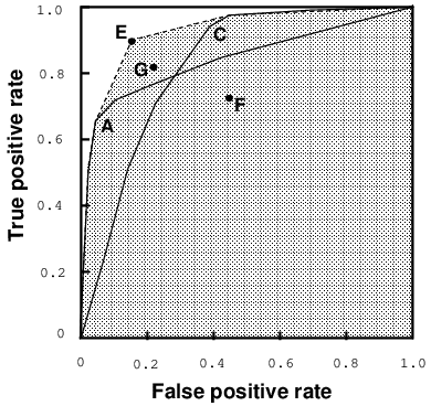
New classifiers can be added incrementally to an rocch analysis, as demonstrated in figure 6 by the addition of classifiers ,, and . Each new classifier either extends the existing hull or it does not. In the former case the hull must be updated accordingly, but in the latter case the new classifier can be ignored. Therefore, the method does not require saving every classifier (or saving statistics on every classifier) for re-analysis under different conditions—only those points on the convex hull. Recall that each point is a classifier and might take up considerable space. Further, the management of knowledge about many classifiers and their statistics from many different runs of learning programs (e.g., with different algorithms or parameter settings) can be a substantial undertaking. Classifiers not on the rocch can never be optimal, so they need not be saved. Every classifier that does lie on the convex hull must be saved. In Section 4.2 we demonstrate the rocch in use, managing the results of many learning experiments.
2.2.5 Changing distributions and costs
Class and cost distributions that change over time necessitate the reevaluation of classifier choice. In fraud detection, costs change based on workforce and reimbursement issues; the amount of fraud changes monthly. With the ROC convex hull method, comparing under a new distribution involves only calculating the slope(s) of the corresponding iso-performance lines and intersecting them with the hull, as shown in figure 4.
The ROC convex hull method scales gracefully to any degree of precision in specifying the cost and class distributions. If nothing is known about a distribution, the ROC convex hull shows all classifiers that may be optimal under any conditions. Figure 3 showed that, given classifiers , , and , only and can ever be optimal. With complete information, the method identifies the optimal classifier(s). In figure 4 we saw that classifier (with a particular threshold value) is optimal under scenario and classifier is optimal under scenario . Next we will see that with less precise information, the ROC convex hull can show the subset of possibly optimal classifiers.
2.2.6 Sensitivity analysis

a. Low sensitivity

b. High sensitivity
Imprecise distribution information defines a range of slopes for iso-performance lines. This range of slopes intersects a segment of the ROC convex hull, which facilitates sensitivity analysis. For example, if the segment defined by a range of slopes corresponds to a single point in ROC space or a small threshold range for a single classifier, then there is no sensitivity to the distribution assumptions in question. Consider a scenario similar to and in that negative examples are 5 times as prevalent as positive ones. In this scenario, consider the cost of dealing with a false alarm to be between $10 and $20, and the cost of missing a positive example to be between $200 and $250. These conditions define a range of slopes for iso-performance lines: . Figure 7a depicts this range of slopes and the corresponding segment of the ROC convex hull. The figure shows that the choice of classifier is insensitive to changes within this range (and only fine tuning of the classifier’s threshold will be necessary). Figure 7b depicts a scenario with a wider range of slopes: . The figure shows that under this scenario the choice of classifier is very sensitive to the distribution. Classifiers , and each are optimal for some subrange.
3 Building robust classifiers
Up to this point, we have concentrated on the use of the rocch for visualizing and evaluating sets of classifiers. The rocch helps to delay classifier selection as long as possible, yet provides a rich performance comparison. However, once system building incorporates a particular classifier, the problem of brittleness resurfaces. This is important because the delay between system building and deployment may be large, and because many systems must survive for years. In fact, in many domains a precise, static specification of future costs and class distributions is not just unlikely, it is impossible [\BCAYProvost, Fawcett, \BBA KohaviProvost et al.1998].
We address this brittleness by using the rocch to produce robust classifiers, defined as satisfying the following. Under any target cost and class distributions, a robust classifier will perform at least as well as the best classifier for those conditions. Our statements about optimality are practical: the “best” classifier may not be the Bayes-optimal classifier, but it is at least as good as any known classifier. Srinivasan \citeyearSrinivasan:99 calls this “FAPP-optimal” (optimal for all practical purposes). Stating that a classifier is robust is stronger than stating that it is optimal for a specific set of conditions. A robust classifier is optimal under all possible conditions.
In principle, classification brittleness could be overcome by saving all possible classifiers (neural nets, decision trees, expert systems, probabilistic models, etc.) and then performing an automated run-time comparison under the desired target conditions. However, such a system is not feasible because of time and space limitations—there are myriad possible classification models, arising from the many different learning methods under their many different parameter settings. Storing all the classifiers is not feasible, and tuning the system by comparing classifiers on the fly under different conditions is not feasible. Fortunately, doing so is not necessary. Moreover, we will show that it is sometimes possible to do better than any of these classifiers.
3.1 ROCCH-hybrid classifiers
We now show that robust hybrid classifiers can be built using the rocch.
Definition 1
Let be the space of possible instances and let be the space of sets of classification models. Let a -hybrid classifier comprise a set of classification models and a function
A -hybrid classifier takes as input an instance for classification and a number . As output, it produces the classification produced by .
Things will get more involved later, but for the time being consider that each set of cost and class distributions defines a value for , which is used to select the (predetermined) best classifier for those conditions. To build a -hybrid classifier, we must define and the set . We would like to include only those models that perform optimally under some conditions (class and cost distributions), since these will be stored by the system, and we would like to be general enough to apply to a variety of problem formulations.
The models comprising the rocch can be combined to form a -hybrid classifier that is an elegant, robust classifier.
Definition 2
The rocch-hybrid is a -hybrid classifier where is the set of classifiers that form the rocch and makes classifications using the classifier on the rocch with .
Note that for the moment the rocch-hybrid is defined only for values corresponding to rocch vertices.
3.2 Robust classification
Our definition of robust classifiers was intentionally vague about what it means for one classifier to be better than another, because different situations call for different comparison frameworks. We now continue with minimizing expected cost, because the process of proving that the rocch-hybrid minimizes expected cost for any cost and class distributions provides a deep understanding of why and how the rocch-hybrid works. Later we generalize to a wide variety of comparison frameworks.
The rocch-hybrid can be seen as an application of multi-criteria optimization to classifier design and construction. The classifiers on the rocch are Edgeworth-Pareto optimal44 4 Edgeworth-Pareto optimality is the century-old notion that in a multidimensional space of criteria, optimal performance is the frontier of achievable performance in this space. In cases where performance is a linear combination of the criteria, the optimality frontier is the convex hull. [\BCAYStadlerStadler1988] with respect to TP, FP, and the objective functions we discuss. Multi-criteria optimization was used previously in machine learning by Tcheng, Lambert, Lu and Rendell \shortciteTchengEtAl:89 for the selection of inductive bias. Alternatively, the rocch can be seen as an application of the theory of games and statistical decisions, for which convex sets (and the convex hull) represent optimal strategies [\BCAYBlackwell \BBA GirshickBlackwell \BBA Girshick1954].
3.2.1 Minimizing expected cost
From above, the expected cost of applying a classifier is:
| (1) |
For a particular set of cost and class distributions, the slope of the corresponding iso-performance lines is:
| (2) |
Every set of conditions will define an . We now can show that the rocch-hybrid is robust for problems where the “best” classifier is the classifier with the minimum expected cost.
The slope of the rocch is an important tool in our argument. The rocch is a piecewise-linear, concave-down “curve.” Therefore, as increases, the slope of the rocch is monotonically non-increasing with discrete values, where is the number of rocch component classifiers, including the degenerate classifiers that define the rocch endpoints. Where there will be no confusion, we use phrases such as “points in ROC space” as a shorthand for the more cumbersome “classifiers corresponding to points in ROC space.” For this subsection, unless otherwise noted, “points on the rocch” refer to vertices of the rocch.
Definition 3
For any real number , the point where the slope of the rocch is is one of the (arbitrarily chosen) endpoints of the segment of the rocch with slope , if such a segment exists. Otherwise, it is the vertex for which the left adjacent segment has slope greater than and the right adjacent segment has slope less than .
For completeness, the leftmost endpoint of the rocch is considered to be attached to a segment with infinite slope and the rightmost endpoint of the rocch is considered to be attached to a segment with zero slope. Note that every defines at least one point on the rocch.
Lemma 1
For any set of cost and class distributions, there is a point on the rocch with minimum expected cost.
Proof: (by contradiction) Assume that for some conditions
there exists a point C with smaller expected cost than any
point on the rocch. By equations 1 and
2, a point (,) has the same expected cost
as a point (,) if
Therefore, for conditions corresponding to , all points with equal expected cost form an iso-performance line in ROC space with slope . Also by 1 and 2, points on lines with larger y-intercept have lower expected cost. Now, point C is not on the rocch, so it is either above the curve or below the curve. If it is above the curve, then the rocch is not a convex set enclosing all points, which is a contradiction. If it is below the curve, then the iso-performance line through C also contains a point P that is on the rocch (not necessarily a vertex). If this iso-performance line intersects no rocch vertex, then consider the vertices at the endpoints of the rocch segment containing P; one of these vertices must intersect a better iso-performance line than does C. In either case, since all points on an iso-performance line have the same expected cost, point C does not have smaller expected cost than all points on the rocch, which is also a contradiction.
Although it is not necessary for our purposes here, it can be shown that all of the minimum expected-cost classifiers are on the rocch.
Definition 4
An iso-performance line with slope is an m-iso-performance line.
Lemma 2
For any cost and class distributions that translate to , a point on
the rocch has minimum expected cost only if the slope
of the rocch at that point is .
Proof: (by contradiction) Suppose that there is a point D
on the rocch where the slope is not , but the point
does have minimum expected cost. By Definition 3,
either (a) the segment to the left of D has slope less than
, or (b) the segment to the right of D has slope greater
than . For case (a), consider point N, the vertex of the
rocch that neighbors D to the left, and consider the
(parallel) -iso-performance lines and through D
and N. Because N is to the left of D and the
line connecting them has slope less than , the y-intercept of
will be greater than the y-intercept of . This means that N
will have lower expected cost than D, which is a contradiction.
The argument for (b) is analogous (symmetric).
Lemma 3
If the slope of the rocch at a point is , then the point has
minimum expected cost.
Proof: If this point is the only point where the slope of the rocch is , then the proof follows directly from Lemma 1 and
Lemma 2. If there are multiple such points, then by definition they are
connected by an -iso-performance line, so they have the same
expected cost, and once again the proof follows directly from Lemma 1 and
Lemma 2.
It is straightforward now to show that the rocch-hybrid is robust for the problem of minimizing expected cost.
Theorem 4
The rocch-hybrid minimizes expected cost for any cost distribution
and any class distribution.
Proof: Because the rocch-hybrid is composed of the
classifiers corresponding to the points on the rocch, this follows
directly from Lemmas 1, 2, and 3.
Now we have shown that the rocch-hybrid is robust when the goal is to provide the minimum expected-cost classification. This result is important even for accuracy maximization, because the preferred classifier may be different for different target class distributions. This rarely is taken into account in experimental comparisons of classifiers.
Corollary 5
The rocch-hybrid minimizes error rate (maximizes accuracy) for any
target class distribution.
Proof: Error rate minimization is cost minimization with uniform
error costs.
3.3 Robust classification for other common metrics
Showing that the rocch-hybrid is robust not only helps us with understanding the rocch method generally, it also shows us how the rocch-hybrid will pick the best classifier in order to produce the best classifications, which we will return to later. If we ignore the need to specify how to pick the best component classifier, we can show that the rocch applies more generally.
Theorem 6
For any classifier evaluation metric , if
and then there exists a
point on the rocch with an -value at least
as high as that of any known classifier.
Proof: (by contradiction) Assume that there exists a classifier
, not on the rocch, with an -value higher than that of
any point on the rocch. is either (i) above or (ii) below
the rocch. In case (i), the rocch is not a convex set enclosing all the
points, which is a contradiction. In case (ii), let be
represented in ROC-space by . Because is below
the rocch there exist points, call one , on the rocch with
and . However, by the restriction on the partial
derivatives, for any such point , which again
is a contradiction.
There are two complications to the more general use of the rocch, both of which are illustrated by the decision criterion from our very first example. Recall that the Neyman-Pearson criterion specifies a maximum acceptable rate. Standard ROC analysis uses ROC curves to select a single, parameterized classification model; the parameter allows the user to select the “operating point” for a decision-making task, usually a threshold on a probabilistic output that will allow for optimal decision making. Under the Neyman-Pearson criterion, selecting the single best model from a set is easy: plot the ROC curves, draw a vertical line at the desired maximum , and pick the model whose curve has the largest at the intersection with this line.

With the rocch-hybrid, making the best classifications under the Neyman-Pearson criterion is not so straightforward. For minimizing expected cost it was sufficient for the rocch-hybrid to choose a vertex from the rocch for any value. For problem formulations such as the Neyman-Pearson criterion, the performance statistics at a non-vertex point on the rocch may be preferable (see figure 8). Fortunately, with a slight extension, the rocch-hybrid can yield a classifier with these performance statistics.
Theorem 7
An rocch-hybrid
can achieve the : tradeoff represented by any point on the
rocch, not just the vertices.
Proof: (by
construction) Extend to non-vertex points as
follows. Pick the point on the rocch with (there
is exactly one). Let be the value of this point. If
(, ) is an rocch vertex, use the corresponding
classifier. If it is not a vertex, call the left endpoint of the
hull segment on which lies , and the right endpoint .
Let be the distance between and , and let be the
distance between and . Make classifications as follows.
For each input instance flip a weighted coin and choose the answer
given by classifier with probability and that
given by classifier with probability . It is
straightforward to show that and for this classifier will
be and .
The second complication is that, as illustrated by the Neyman-Pearson criterion, many practical classifier comparison frameworks include constrained optimization problems (below we will discuss other frameworks). Arbitrarily constrained optimizations are problematic for the rocch-hybrid. Given total freedom, it is possible to devise constraints on classifier performance such that, even with the restriction on the partial derivatives, an interior point scores higher than any acceptable point on the hull. For example, two linear constraints can enclose a subset of the interior and exclude the entire rocch—there will be no acceptable points on the rocch. However, many realistic constraints do not thwart the optimality of the rocch-hybrid.
Theorem 8
For any classifier evaluation metric , if
and and no constraint on
classifier performance eliminates any point on the rocch without also
eliminating all higher-scoring interior points, then the rocch-hybrid can
perform at least as well as any known classifier.
Proof: Follows directly from Theorem 6
and Theorem 7.
Linear constraints on classifiers’ performance are common for real-world problems, so the following is useful.
Corollary 9
For any classifier evaluation metric , if
and
and there is a single constraint on classifier performance
of the form , with and
non-negative,
then
the rocch-hybrid can perform at least as well as any known
classifier.
Proof:
The single constraint eliminates from contention all points (classifiers)
that do not fall to the left of, or below, a line with non-positive
slope. By the restriction on the partial derivatives, such a constraint
will not eliminate a point on the rocch without also eliminating
all interior points with higher -values.
Thus, the proof follows directly from Theorem 8.
So, finally, we have the following:
Corollary 10
For the Neyman-Pearson criterion, the rocch-hybrid can perform at
least as well as that of any known
classifier.
Proof: For the Neyman-Pearson criterion, the evaluation metric is
, that is, a higher is better. The constraint on
classifier performance is . These satisfy the conditions
for Corollary 9, and therefore this
corollary follows.
All the foregoing effort may seem misplaced for a simple criterion like Neyman-Pearson. However, there are many other realistic problem formulations. For example, consider the decision-support problem of optimizing workforce utilization, in which a workforce is available that can process a fixed number of cases. Too few cases will under-utilize the workforce, but too many cases will leave some cases unattended (expanding the workforce usually is not a short-term solution). If the workforce can handle cases, the system should present the best possible set of cases. This is similar to the Neyman-Pearson criterion, but with an absolute cutoff () instead of a percentage cutoff ().
Theorem 11
For workforce utilization, the rocch-hybrid will provide the best set
of cases, for any choice of .
Proof: (by construction) The decision criterion is to maximize
subject to the constraint:
The theorem therefore follows from Corollary 9.
In fact, many screening problems, such as are found in marketing and information retrieval, use exactly this linear constraint. It follows that for maximizing lift [\BCAYBerry \BBA LinoffBerry \BBA Linoff1997], precision, or recall, subject to absolute or percentage cutoffs on case presentation, the rocch-hybrid will provide the best set of cases.
As with minimizing expected cost, imprecision in the environment forces us to favor a robust solution for these other comparison frameworks. For many real-world problems, the precise desired cutoff will be unknown or will change (e.g., because of fundamental uncertainty, variability in case difficulty, or competing responsibilities). What is worse, for a fixed (absolute) cutoff merely changing the size of the universe of cases (e.g., the size of a document corpus) may change the preferred classifier, because it will change the constraint line. The rocch-hybrid provides a robust solution because it gives the optimal subset of cases for any constraint line. For example, for document retrieval the rocch-hybrid will yield the best documents for any , for any prior class distribution (in the target corpus), and for any target corpus size.
3.4 Ranking cases
An apparent solution to the problem of robust classification is to use a model that ranks cases, and just work down the ranked list. This approach appears to sidestep the brittleness demonstrated with binary classifiers, since the choice of a cutoff point can be deferred to classification time. However, choosing the best ranking model is still problematic. For most practical situations, choosing the best ranking model is equivalent to choosing which classifier is best for the cutoff that will be used.
An example will illustrate this. Consider two ranking functions, and , applied to a class-balanced set of 100 cases. Assume is able to recognize a common aspect unique to positive cases that occurs in 20% of the population, and it ranks these highest. Assume is able to recognize a common aspect unique to negative cases occurring in 20% of the population, and it ranks these lowest. So ranks the highest 20% correctly and performs randomly on the remainder, while ranks the lowest 20% correctly and performs randomly on the remainder. Which model is better? The answer depends entirely upon how far down the list the system will go before it stops; that is, upon what cutoff will be used. If fewer than 50 cases are to be selected then should be used, whereas is better if more than 50 cases will be selected. Figure 9 shows the ROC curves corresponding to these two classifiers, and the point corresponding to where the curves cross in ROC space.

The rocch method can be used to organize such ranking models, as we have seen. Recall that ROC curves are formed from case rankings by moving the cutoff from one extreme to the other (Table 1 shows an algorithm for calculating the ROC curve from such rankings). The rocch-hybrid comprises the ranking models that are best for all possible conditions.
3.5 Whole-curve metrics
In situations where either the target cost distribution or class distribution is completely unknown, some researchers advocate choosing the classifier that maximizes a single-number metric representing the average performance over the entire curve. A common whole-curve metric is “AUC”, the Area Under the (ROC) Curve [\BCAYBradleyBradley1997]. The AUC is equivalent to the probability that a randomly chosen positive instance will be rated higher than a negative instance, and thereby is also estimated by the Wilcoxon test of ranks [\BCAYHanley \BBA McNeilHanley \BBA McNeil1982]. A criticism of AUC is that for specific target conditions the classifier with the maximum AUC may be suboptimal [\BCAYProvost, Fawcett, \BBA KohaviProvost et al.1998]. Indeed, this criticism may be made of any single-number metric. Fortunately, not only is the rocch-hybrid optimal for any specific target conditions, it has the maximum AUC—There is no classifier with AUC larger than that of the rocch-hybrid.
3.6 Using the ROCCH-hybrid
To use the rocch-hybrid for classification, we need to translate environmental conditions to values to plug into . For minimizing expected cost, Equation 2 shows how to translate conditions to . For any , by Lemma 3 we want the value of the point where the slope of the rocch is , which is straightforward to calculate. For the Neyman-Pearson criterion the conditions are defined as values. For workforce utilization with conditions corresponding to a cutoff , the value is found by intersecting the line with the rocch.
We have argued that target conditions (misclassification costs and class distribution) are rarely known. It may be confusing that we now seem to require exact knowledge of these conditions. The rocch-hybrid gives us two important capabilities. First, the need for precise knowledge of target conditions is deferred until run time. Second, in the absence of precise knowledge even at run time, the system can be optimized easily with minimal feedback.
By using the rocch-hybrid, information on target conditions is not needed to train and compare classifiers. This is important because of imprecision caused by temporal, geographic, or other differences that may exist between training and use. For example, building a system for a real-world problem introduces a non-trivial delay between the time data are gathered and the time the learned models will be used. The problem is exacerbated in domains where error costs or class distributions change over time; even with slow drift, a brittle model may become suboptimal quickly. In many such scenarios, costs and class distributions can be specified (or respecified) at run time with reasonable precision by sampling from the current population, and used to ensure that the rocch-hybrid always performs optimally.
In some cases, even at run time these quantities are not known exactly. A further benefit of the rocch-hybrid is that it can be tuned easily to yield optimal performance with only minimal feedback from the environment. Conceptually, the rocch-hybrid has one “knob” that varies in from one extreme to the other. For any knob setting, the rocch-hybrid will give the optimal : tradeoff for the target conditions corresponding to that setting. Turning the knob to the right increases ; turning the knob to the left decreases . Because of the monotonicity of the rocch-hybrid, simple hill-climbing can guarantee optimal performance. For example, if the system produces too many false alarms, turn the knob to the left; if the system is presenting too few cases, turn the knob to the right.
3.7 Beating the component classifiers
Perhaps surprisingly, in many realistic situations an rocch-hybrid system can do better than any of its component classifiers. Consider the Neyman-Pearson decision criterion. The rocch may intersect the -line above the highest component ROC curve. This occurs when the -line intersects the rocch between vertices; therefore, there is no component classifier that actually produces these particular (,) statistics, as in figure 8. By Theorem 7, the rocch-hybrid can achieve any on the hull. Only a small number of values correspond to hull vertices. The same holds for other common problem formulations, such as workforce utilization, lift maximization, precision maximization, and recall maximization.
3.8 Time and space efficiency
We have argued that the rocch-hybrid is robust for a wide variety of problem formulations. It is also efficient to build, to store, and to update.
The time efficiency of building the rocch-hybrid depends first on the efficiency of building the component models, which varies widely by model type. Some models built by machine learning methods can be built in seconds (once data are available). Hand-built models can take years to build. However, we presume that this is work that would be done anyway. The rocch-hybrid can be built with whatever methods are available, be there two or two thousand. As described below, as new classifiers become available, the rocch-hybrid can be updated incrementally. The time efficiency depends also on the efficiency of the experimental evaluation of the classifiers. Once again, we presume that this is work that would be done anyway. Finally, the time efficiency of the rocch-hybrid depends on the efficiency of building the rocch, which can be done in time using the QuickHull algorithm [\BCAYBarber, Dobkin, \BBA HuhdanpaaBarber et al.1996] where is the number of classifiers.
The rocch is space efficient, too, because it comprises only classifiers that might be optimal under some target conditions (which follows directly from Lemmas 1–3 and Definitions 3 and 4). The number of classifiers that must be stored can be reduced if bounds can be placed on the potential target conditions. As described above, ranges of conditions define segments of the rocch. Thus, the rocch-hybrid may need only a subset of .
Adding new classifiers to the rocch-hybrid also is efficient. Adding a classifier to the rocch will either (i) extend the hull, adding to (and possibly subtracting from) the rocch-hybrid, or (ii) conclude that the new classifiers are not superior to the existing classifiers in any portion of ROC space and can be discarded.
The run-time (classification) complexity of the rocch-hybrid is never worse than that of the component classifiers. In situations where run-time complexity is crucial, the rocch should be constructed without prohibitively expensive classification models. It then will find the best subset of the computationally efficient models.
4 Empirical demonstration of need
Robust classification is of fundamental interest because it weakens two very strong assumptions: the availability of precise knowledge of costs and of class distributions. However, might it not be that existing classifiers already are robust? For example, if a given classifier is optimal under one set of conditions, might it not be optimal under all?
It is beyond the scope of this paper to offer an in-depth experimental study answering this question. However, we can provide solid evidence that the answer is “no” by referring to the results of two prior studies. One is a comprehensive ROC analysis of medical domains recently conducted by Andrew Bradley \citeyearBradley:97.55 5 Bradley’s purpose was not to answer this question; fortunately, his published results do anyway. The other is a published ROC analysis of UCI database domains that we undertook last year with Ron Kohavi [\BCAYProvost, Fawcett, \BBA KohaviProvost et al.1998].
Note that a classifier dominates if its ROC curve completely defines the rocch (which means dominating classifiers are robust and vice versa). Therefore, if there exist more than a trivially few domains where no single classifier dominates, then techniques like the rocch-hybrid are essential if robust classifiers are desired.
4.1 Bradley’s study
Bradley studied six medical data sets, noting that “unfortunately, we rarely know what the individual misclassification costs are.” He plotted the ROC curves of six classifier learning algorithms (two neural nets, two decision trees and two statistical techniques).

On not one of these data sets was there a dominating classifier. This means that for each domain, there exist different sets of conditions for which different classifiers are preferable. In fact, the running example in the present article is based on the three best classifiers from Bradley’s results on the heart bleeding data; his results for the full set of six classifiers can be found in figure 10. Classifiers constructed for the Cleveland heart disease data are shown in figure 11.
Bradley’s results show clearly that for many domains the classifier that maximizes any single metric—be it accuracy, cost, or the area under the ROC curve—will be the best for some cost and class distributions and will not be the best for others. We have shown that the rocch-hybrid will be the best for all.

4.2 Our study
In the study we performed with Ron Kohavi, we chose ten datasets from the UCI repository, each of which contains at least 250 instances, but for which the accuracy for decision trees was less than 95%. For each domain, we induced classifiers for the minority class (for Road, we chose the class Grass). We selected several induction algorithms from [\BCAYKohavi, Sommerfield, \BBA DoughertyKohavi et al.1997]: a decision tree learner (MC4), Naive Bayes with discretization (NB), -nearest neighbor for several values (IB), and Bagged-MC4 [\BCAYBreimanBreiman1996]. MC4 is similar to C4.5 [\BCAYQuinlanQuinlan1993]; probabilistic predictions are made by using a Laplace correction at the leaves. NB discretizes the data based on entropy minimization [\BCAYDougherty, Kohavi, \BBA SahamiDougherty et al.1995] and then builds the Naive-Bayes model [\BCAYDomingos \BBA PazzaniDomingos \BBA Pazzani1997]. IB votes the closest neighbors; each neighbor votes with a weight equal to one over its distance from the test instance.
Some of the ROC curves are shown in Figure 12. For only one of these ten domains (Vehicle) was there an absolute dominator. In general, very few of the 100 runs performed (on 10 data sets, using 10 cross-validation folds each) had dominating classifiers. Some cases are very close, for example Adult and Waveform-21. In other cases a curve that dominates in one area of ROC space is dominated in another. These results also support the need for methods like the rocch-hybrid, which produce robust classifiers.

 a. Vehicle
b. CRX
a. Vehicle
b. CRX

 c. RoadGrass
d. Satimage
c. RoadGrass
d. Satimage
| Domain | Slope range | Dominator |
| Vehicle | [0, ) | Bagged-MC4 |
| Road (Grass) | [0, 0.38] | NB |
| [0.38, ) | Bagged-MC4 | |
| CRX | [0, 0.03] | Bagged-MC4 |
| [0.03, 0.06] | NB | |
| [0.06, 2.06] | Bagged-MC4 | |
| [2.06, ) | NB | |
| Satimage | [0, 0.05] | NB |
| [0.05, 0.22] | Bagged-MC4 | |
| [0.22, 2.60] | IB5 | |
| [2.60, 3.11] | IB3 | |
| [3.11, 7.54] | IB5 | |
| [7.54, 31.14] | IB3 | |
| [31.14, ) | Bagged-MC4 |
As examples of what expected-cost-minimizing rocch-hybrids would look like internally, Table 2 shows the component classifiers that make up the rocch for the four UCI domains of figure 12. For example, in the Road domain (see figure 12 and Table 2), Naive Bayes would be chosen for any target conditions corresponding to a slope less than , and Bagged-MC4 would be chosen for slopes greater than . They perform equally well at .
5 Limitations and future work
There are limitations to the rocch method as we have presented it here. We have defined it here only for two-class problems. Srinivasan \citeyearSrinivasan:99 shows that it can be extended to multiple dimensions. It should be noted that the dimensionality of the “ROC-hyperspace” grows quadratically in the number of classes, so both efficiency and visualization capability are called into question.
We have assumed constant error costs for a given type of error, e.g., all false positives cost the same. For some problems, different errors of the same type have different costs. In many cases, such a problem can be transformed for evaluation into an equivalent problem with uniform intra-type error costs by duplicating instances in proportion to their costs (or by simply modifying the counting procedure accordingly).
We also have assumed for this paper that the estimates of the classifiers’ performance statistics ( and ) are very good. As mentioned above, much work has addressed the production of good estimates for simple performance statistics such as error rate. Much less work has addressed the production of good ROC curve estimates. As with simpler statistics, care should be taken to avoid over-fitting the training data and to ensure that differences between ROC curves are meaningful. One solution is to use cross-validation with averaging of ROC curves [\BCAYProvost, Fawcett, \BBA KohaviProvost et al.1998], which is the procedure used to produce the ROC curves in Section 4.2. To our knowledge, the issue is open of how best to produce confidence bands appropriate to a particular problem. Those shown in Section 4.2 are appropriate for the Neyman-Pearson decision criterion (i.e., they show confidence on for various values of ).
Also, we have addressed predictive performance and computational performance. These are not the only concerns in choosing a classification model. What if comprehensibility is important? The easy answer is that for any particular setting, the rocch-hybrid is as comprehensible as the underlying model it is using. However, this answer falls short if the rocch-hybrid is interpolating between two models or if one wants to understand the “multiple-model” system as a whole.
Although ROC analysis and the ROCCH method were specifically designed for classification domains, we have extended them to activity monitoring domains [\BCAYFawcett \BBA ProvostFawcett \BBA Provost1999]. Such domains involve monitoring the behavior of a population of entities for interesting events requiring action. These problems are substantially different from standard classification because timeliness of classification is important and dependencies exist among instances; both factors complicate evaluation.
This work is fundamentally different from other recent machine learning work on combining multiple models [\BCAYAli \BBA PazzaniAli \BBA Pazzani1996]. That work combines models in order to boost performance for a fixed cost and class distribution. The rocch-hybrid combines models for robustness across different cost and class distributions. In principle, these methods should be independent—multiple-model classifiers are candidates for extending the rocch. However, it may be that some multiple-model classifiers achieve increased performance for a specific set of conditions by (in effect) interpolating along edges of the rocch. Cherikh [\BCAYCherikhCherikh1989] uses ROC analysis to study decision making where the decisions of multiple models are present. Unlike our work, the goal is to find optimal combinations of models for specific conditions. However, it seems that the two methods may be combined profitably: well-chosen combinations of models should extend the ROCCH, yielding a better robust classifier.
The rocch method also complements research on cost-sensitive learning [\BCAYTurneyTurney1996]. Existing cost-sensitive learning methods are brittle with respect to imprecise cost knowledge. Thus, the rocch is an essential evaluation tool. Furthermore, cost-sensitive learning may be used to find better components for the rocch-hybrid, by searching explicitly for classifiers that extend the rocch.
6 Conclusion
The ROC convex hull method is a robust, efficient solution to the problem of comparing multiple classifiers in imprecise and changing environments. It is intuitive, can compare classifiers both in general and under specific distribution assumptions, and provides crisp visualizations. It minimizes the management of classifier performance data, by selecting exactly those classifiers that are potentially optimal; thus, only these need to be saved in preparation for changing conditions. Moreover, due to its incremental nature, new classifiers can be incorporated easily, e.g., when trying a new parameter setting.
The rocch-hybrid performs optimally under any target conditions for many realistic problem formulations, including the optimization of metrics such as accuracy, expected cost, lift, precision, recall, and workforce utilization. It is efficient to build in terms of time and space, and can be updated incrementally. Furthermore, it can sometimes classify better than any (other) known model. Therefore, we conclude that it is an elegant, robust classification system.
We believe that this work has important implications for both machine learning applications and machine learning research [\BCAYProvost, Fawcett, \BBA KohaviProvost et al.1998]. For applications, it helps free system designers from the need to choose (sometimes arbitrary) comparison metrics before precise knowledge of key evaluation parameters is available. Indeed, such knowledge may never be available, yet robust systems still can be built.
For machine learning research, it frees researchers from the need to have precise class and cost distribution information in order to study important related phenomena. In particular, work on cost-sensitive learning has been impeded by the difficulty of specifying costs, and by the tenuous nature of conclusions based on a single cost metric. Researchers need not be held back by either. Cost-sensitive learning can be studied generally without specifying costs precisely. The same goes for research on learning with highly skewed distributions. Which methods are effective for which levels of distribution skew? The rocch will provide a detailed answer.
Recently, Drummond and Holte [\BCAYDrummond \BBA HolteDrummond \BBA Holte2000] have demonstrated an intriguing dual to the rocch. Their “cost curves” represent expected costs explicitly, rather than as slopes of iso-performance lines, and thereby provide an insightful alternative perspective for visualization.
Note: An implementation of the rocch method in Perl is publicly available. The code and related papers may be found at: http://www.hpl.hp.com/personal/Tom_Fawcett/ROCCH/.
7 Acknowledgments
Much of this work was done while the authors were employed at the Bell Atlantic Science and Technology Center. We thank the many with whom we have discussed ROC analysis and classifier comparison, especially Rob Holte, George John, Ron Kohavi, Ron Rymon, and Peter Turney. We thank Andrew Bradley for supplying data from his analysis.
References
- [\BCAYAli \BBA PazzaniAli \BBA Pazzani1996] Ali, K. M.\BBACOMMA \BBA Pazzani, M. J. \BBOP1996\BBCP. \BBOQError Reduction through Learning Multiple Descriptions\BBCQ \BemMachine Learning, \Bem24(3), 173–202.
- [\BCAYBarber, Dobkin, \BBA HuhdanpaaBarber et al.1996] Barber, C. B., Dobkin, D. P., \BBA Huhdanpaa, H. \BBOP1996\BBCP. \BBOQThe quickhull algorithm for convex hulls\BBCQ \BemACM Transactions on Mathematical Software, \Bem22(4), 469–483. Available from http://www.acm.org/pubs/citations/journals/toms/1996-22-4/p469-barber/.
- [\BCAYBeck \BBA SchultzBeck \BBA Schultz1986] Beck, J. R.\BBACOMMA \BBA Schultz, E. K. \BBOP1986\BBCP. \BBOQThe Use of ROC Curves in Test Performance Evaluation\BBCQ \BemArch Pathol Lab Med, \Bem110, 13–20.
- [\BCAYBerry \BBA LinoffBerry \BBA Linoff1997] Berry, M. J. A.\BBACOMMA \BBA Linoff, G. \BBOP1997\BBCP. \BemData Mining Techniques: For Marketing, Sales, and Customer Support. John Wiley & Sons.
- [\BCAYBlackwell \BBA GirshickBlackwell \BBA Girshick1954] Blackwell, D.\BBACOMMA \BBA Girshick, M. A. \BBOP1954\BBCP. \BemTheory of Games and Statistical Decisions. John Wiley and Sons, Inc. Republished by Dover Publications, New York, in 1979.
- [\BCAYBradleyBradley1997] Bradley, A. P. \BBOP1997\BBCP. \BBOQThe use of the area under the ROC curve in the evaluation of machine learning algorithms\BBCQ \BemPattern Recognition, \Bem30(7), 1145–1159.
- [\BCAYBreiman, Friedman, Olshen, \BBA StoneBreiman et al.1984] Breiman, L., Friedman, J., Olshen, R., \BBA Stone, C. \BBOP1984\BBCP. \BemClassification and regression trees. Wadsworth International Group, Belmont, CA.
- [\BCAYBreimanBreiman1996] Breiman, L. \BBOP1996\BBCP. \BBOQBagging Predictors\BBCQ \BemMachine Learning, \Bem24, 123–140.
- [\BCAYCatlettCatlett1995] Catlett, J. \BBOP1995\BBCP. \BBOQTailoring rulesets to misclassification costs\BBCQ In \BemProceedings of the Fifth International Workshop on Artificial Intelligence and Statistics, \BPGS 88–94.
- [\BCAYCherikhCherikh1989] Cherikh, M. \BBOP1989\BBCP. \BemOptimal decision and detection in the decentralized case. Ph.D. thesis, Case Western Reserve University.
- [\BCAYClearwater \BBA SternClearwater \BBA Stern1991] Clearwater, S.\BBACOMMA \BBA Stern, E. \BBOP1991\BBCP. \BBOQA rule-learning program in high energy physics event classification\BBCQ \BemComp Physics Comm, \Bem67, 159–182.
- [\BCAYDietterichDietterich1998] Dietterich, T. G. \BBOP1998\BBCP. \BBOQApproximate Statistical Tests for Comparing Supervised Classification Learning Algorithms\BBCQ \BemNeural Computation, \Bem10(7), 1895–1924.
- [\BCAYDomingosDomingos1999] Domingos, P. \BBOP1999\BBCP. \BBOQMetaCost: A general method for making classifiers cost-sensitive\BBCQ In \BemProceedings of the Fifth ACM SIGKDD International Conference on Knowledge Discovery and Data Mining, \BPGS 155–164.
- [\BCAYDomingos \BBA PazzaniDomingos \BBA Pazzani1997] Domingos, P.\BBACOMMA \BBA Pazzani, M. \BBOP1997\BBCP. \BBOQBeyond Independence: Conditions for the Optimality of the Simple Bayesian Classifier\BBCQ \BemMachine Learning, \Bem29, 103–130.
- [\BCAYDougherty, Kohavi, \BBA SahamiDougherty et al.1995] Dougherty, J., Kohavi, R., \BBA Sahami, M. \BBOP1995\BBCP. \BBOQSupervised and Unsupervised Discretization of Continuous Features\BBCQ In Prieditis, A.\BBACOMMA \BBA Russell, S.\BEDS, \BemProceedings of the Twelfth International Conference on Machine Learning, \BPGS 194–202 San Francisco. Morgan Kaufmann.
- [\BCAYDrummond \BBA HolteDrummond \BBA Holte2000] Drummond, C.\BBACOMMA \BBA Holte, R. C. \BBOP2000\BBCP. \BBOQExplicitly Representing Expected Cost: An Alternative to ROC Representation\BBCQ In Ramakrishnan, R.\BBACOMMA \BBA Stolfo, S.\BEDS, \BemProceedings on the Sixth ACM SIGKDD International Conference on Knowledge Discovery and Data Mining.
- [\BCAYEganEgan1975] Egan, J. P. \BBOP1975\BBCP. \BemSignal Detection Theory and ROC Analysis. Series in Cognitition and Perception. Academic Press, New York.
- [\BCAYEzawa, Singh, \BBA NortonEzawa et al.1996] Ezawa, K., Singh, M., \BBA Norton, S. \BBOP1996\BBCP. \BBOQLearning Goal Oriented Bayesian Networks for Telecommunications Risk Management\BBCQ In Saitta, L.\BED, \BemProceedings of the Thirteenth International Conference on Machine Learning, \BPGS 139–147 San Francisco, CA. Morgan Kaufmann.
- [\BCAYFawcett \BBA ProvostFawcett \BBA Provost1996] Fawcett, T.\BBACOMMA \BBA Provost, F. \BBOP1996\BBCP. \BBOQCombining Data Mining and Machine Learning for Effective User Profiling\BBCQ In Simoudis, Han, \BBA Fayyad\BEDS, \BemProceedings on the Second International Conference on Knowledge Discovery and Data Mining, \BPGS 8–13 Menlo Park, CA. AAAI Press.
- [\BCAYFawcett \BBA ProvostFawcett \BBA Provost1997] Fawcett, T.\BBACOMMA \BBA Provost, F. \BBOP1997\BBCP. \BBOQAdaptive Fraud Detection\BBCQ \BemData Mining and Knowledge Discovery, \Bem1(3), 291–316.
- [\BCAYFawcett \BBA ProvostFawcett \BBA Provost1999] Fawcett, T.\BBACOMMA \BBA Provost, F. \BBOP1999\BBCP. \BBOQActivity monitoring: Noticing interesting changes in behavior\BBCQ In Chaudhuri\BBACOMMA \BBA Madigan\BEDS, \BemProceedings on the Fifth ACM SIGKDD International Conference on Knowledge Discovery and Data Mining, \BPGS 53–62.
- [\BCAYFriedman \BBA WyattFriedman \BBA Wyatt1997] Friedman, C. P.\BBACOMMA \BBA Wyatt, J. C. \BBOP1997\BBCP. \BemEvaluation Methods in Medical Informatics. Springer-Verlag, New York.
- [\BCAYHanley \BBA McNeilHanley \BBA McNeil1982] Hanley, J. A.\BBACOMMA \BBA McNeil, B. J. \BBOP1982\BBCP. \BBOQThe Meaning and Use of the Area under a Receiver Operating Characteristic (ROC) Curve\BBCQ \BemRadiology, \Bem143, 29–36.
- [\BCAYKlinkenberg \BBA ThorstenKlinkenberg \BBA Thorsten2000] Klinkenberg, R.\BBACOMMA \BBA Thorsten, J. \BBOP2000\BBCP. \BBOQDetecting Concept Drift with Support Vector Machines\BBCQ In \BemProceedings of the Seventeenth International Conference on Machine Learning San Francisco. Morgan Kaufmann.
- [\BCAYKohaviKohavi1995] Kohavi, R. \BBOP1995\BBCP. \BBOQA Study of Cross-Validation and Bootstrap for Accuracy Estimation and Model Selection\BBCQ In Mellish, C. S.\BED, \BemProceedings of the 14th International Joint Conference on Artificial Intelligence, \BPGS 1137–1143 San Francisco. Morgan Kaufmann.
- [\BCAYKohavi, Sommerfield, \BBA DoughertyKohavi et al.1997] Kohavi, R., Sommerfield, D., \BBA Dougherty, J. \BBOP1997\BBCP. \BBOQData Mining Using : A Machine Learning Library in C++\BBCQ \BemInternational Journal on Artificial Intelligence Tools, \Bem6(4), 537–566. Available: http://www.sgi.com/Technology/mlc.
- [\BCAYKubat, Holte, \BBA MatwinKubat et al.1998] Kubat, M., Holte, R., \BBA Matwin, S. \BBOP1998\BBCP. \BBOQMachine Learning for the Detection of Oil Spills in Satellite Radar Images\BBCQ \BemMachine Learning, \Bem30(2/3), 195–215.
- [\BCAYPazzani, Merz, Murphy, Ali, Hume, \BBA BrunkPazzani et al.1994] Pazzani, M., Merz, C., Murphy, P., Ali, K., Hume, T., \BBA Brunk, C. \BBOP1994\BBCP. \BBOQReducing misclassification costs\BBCQ In \BemProceedings of the Eleventh International Conference on Machine Learning, \BPGS 217–225 San Francisco. Morgan Kaufmann.
- [\BCAYProvost \BBA FawcettProvost \BBA Fawcett1997] Provost, F.\BBACOMMA \BBA Fawcett, T. \BBOP1997\BBCP. \BBOQAnalysis and Visualization of Classifier Performance: Comparison under imprecise class and cost distributions\BBCQ In \BemProceedings of the Third International Conference on Knowledge Discovery and Data Mining, \BPGS 43–48 Menlo Park, CA. AAAI Press, AAAI Press.
- [\BCAYProvost, Fawcett, \BBA KohaviProvost et al.1998] Provost, F., Fawcett, T., \BBA Kohavi, R. \BBOP1998\BBCP. \BBOQThe Case Against Accuracy Estimation for Comparing Induction Algorithms\BBCQ In Shavlik, J.\BED, \BemProceedings of the Fifteenth International Conference on Machine Learning, \BPGS 445–453 San Francisco, CA. Morgan Kaufmann.
- [\BCAYQuinlanQuinlan1993] Quinlan, J. R. \BBOP1993\BBCP. \BemC4.5: Programs for Machine Learning. Morgan Kaufmann, San Francisco, CA.
- [\BCAYSaitta \BBA NeriSaitta \BBA Neri1998] Saitta, L.\BBACOMMA \BBA Neri, F. \BBOP1998\BBCP. \BBOQLearning in the “Real World”\BBCQ \BemMachine Learning, \Bem30, 133–163.
- [\BCAYSalzbergSalzberg1997] Salzberg, S. L. \BBOP1997\BBCP. \BBOQOn Comparing Classifiers: Pitfalls to Avoid and a Recommended Approach\BBCQ \BemData Mining and Knowledge Discovery, \Bem1, 317–328.
- [\BCAYSrinivasanSrinivasan1999] Srinivasan, A. \BBOP1999\BBCP. \BBOQNote on the Location of Optimal Classifiers in ROC Space\BBCQ Technical report PRG-TR-2-99, Oxford University.
- [\BCAYStadlerStadler1988] Stadler, W.\BED. \BBOP1988\BBCP. \BemMulticriteria Optimization in Engineering and in the Sciences. New York: Plenum Press.
- [\BCAYSwetsSwets1988] Swets, J. \BBOP1988\BBCP. \BBOQMeasuring the accuracy of diagnostic systems\BBCQ \BemScience, \Bem240, 1285–1293.
- [\BCAYTcheng, Lambert, Lu, \BBA RendellTcheng et al.1989] Tcheng, D., Lambert, B., Lu, S. C.-Y., \BBA Rendell, L. \BBOP1989\BBCP. \BBOQBuilding robust learning systems by computing induction and optimization\BBCQ In Sridharan, N. S.\BED, \BemProceedings of the Eleventh International Joint Conference on Artificial Intelligence, \BPGS 806–812 San Francisco, CA. Morgan Kaufmann.
- [\BCAYTurneyTurney1996] Turney, P. \BBOP1996\BBCP. \BBOQCost Sensitive Learning Bibliography\BBCQ Available: http://ai.iit.nrc.ca/bibliographies/cost-sensitive.html.
- [\BCAYWeinstein \BBA FinebergWeinstein \BBA Fineberg1980] Weinstein, M. C.\BBACOMMA \BBA Fineberg, H. V. \BBOP1980\BBCP. \BemClinical Decision Analysis. Philadelphia, PA: W. B. Saunders Company.
- [\BCAYZahavi \BBA LevinZahavi \BBA Levin1997] Zahavi, J.\BBACOMMA \BBA Levin, N. \BBOP1997\BBCP. \BBOQIssues and Problems in Applying Neural Computing to Target Marketing\BBCQ \BemJournal of Direct Marketing, \Bem11(4), 63–75.