Flipturning PolygonsThanks: Portions of this work were done at the Workshop on Polygonal Entanglement Theory held February 4–11, 2000 at McGill University’s Bellairs Research Center, Holetown, Barbados. For the most recent version of this paper, see http://www.uiuc.edu/~jeffe/pubs/flipturn.html.
A flipturn is an operation that transforms a nonconvex simple polygon into another simple polygon, by rotating a concavity 180 degrees around the midpoint of its bounding convex hull edge. Joss and Shannon proved in 1973 that a sequence of flipturns eventually transforms any simple polygon into a convex polygon. This paper describes several new results about such flipturn sequences. We show that any orthogonal polygon is convexified after at most arbitrary flipturns, or at most well-chosen flipturns, improving the previously best upper bound of . We also show that any simple polygon can be convexified by at most flipturns, generalizing earlier results of Ahn et al. These bounds depend critically on how degenerate cases are handled; we carefully explore several possibilities. We describe how to maintain both a simple polygon and its convex hull in time per flipturn, using a data structure of size . We show that although flipturn sequences for the same polygon can have significantly different lengths, the shape and position of the final convex polygon is the same for all sequences and can be computed in time. Finally, we demonstrate that finding the longest convexifying flipturn sequence of a simple polygon is NP-hard.
1 Introduction
A central problem in polymer physics and molecular biology is the reconfiguration of large molecules (modeled as polygons) such as circular DNA [12]. Most of the research in this area involves computer-intensive Monte-Carlo simulations. To simplify these simulations they are usually restricted to the integer lattices and , although some work has also been done on the FCC lattice [21]. Like the related algorithmic robotics research on linkages, the problems of interest to physicists and biologists involve closed simple polygons [8], open simple polygonal chains [18] and simple polygonal trees [11], i.e., polygons, chains, and trees that do not intersect themselves; hence the term self-avoiding walks for the case of polygons and chains. Generating a random self-avoiding walk from scratch is difficult, especially if it must return to its starting point as in the case of polygons. The waiting time is too long due to attrition; if a random walk crosses itself at any point other than its starting point, it must be discarded and a new walk started. Therefore an efficient method frequently used to generate random chains or polygons is to modify one such object into another using a simple operation called a pivot. Unlike the work in linkages, however, here we do not care if intersections happen during the pivot as long as when the pivot is complete we end up with a simple polygon or chain. In other words, pivots are seen as instantaneous combinatorial changes, not continuous processes. In general the pivots used are selected from a large variety of transformations such as reflections, rotations, or ‘cut and paste’ operations on certain subchains. We refer the reader to a multitude of such problems and results in [16]. For example, Madras and Sokal [17] have shown that for all , every simple lattice polygonal chain with edges in can be straightened by some sequence of at most suitable pivots while maintaining simplicity after each pivot. The pivots used here are either reflections through coordinate hyperplanes or rotations by right angles.
In order to prove the ergodicity of their self-avoiding walks, polymer physicists are interested in convexifying polygons (and straightening open polygonal chains). If a polygon can be transformed to some canonical convex configuration, then any simple polygon can be reconfigured to any other via this intermediate position. This theoretical aspect of polymer physics research resembles the algorithmic robotics work on convexification of polygonal linkages. We refer the reader to survey papers of O’Rourke [19] and Toussaint [25] for further references in the latter area.
In this paper, we are concerned with one type of pivot of central concern in polymer physics research. This pivot is usually called an inversion in the physics literature, but since it seems to have been first proposed in an unpublished 1973 paper of Joss and Shannon [13], we will follow their terminology and call it a flipturn. Flipturns are defined as follows. Any nonconvex polygon has at least one concavity, or pocket. Formally, a pocket of a nonconvex polygon is a maximal connected sequence of polygon edges disjoint from the convex hull of except at its endpoints. The line segment joining the endpoints of a pocket is called the lid of the pocket. A flipturn rotates a pocket 180 degrees about the midpoint of its lid, or equivalently, reverses the order of the edges of a pocket without changing their lengths or orientations. Figure 1.1 shows the effect of a single flipturn on a nonconvex orthogonal polygon, and Figure 1.2 shows a sequence of flipturns transforming this polygon into a rectangle. We will illustrate such sequences by overlaying the resulting polygons and labeling the area added by each flipturn by its position in the sequence. (The circled numbers will be explained in Section 2.)


1.1 Previous and Related Results
Joss and Shannon proved that any simple polygon with sides can be convexified by a sequence of at most flipturns, by observing that each flipturn produces a new cyclic permutation of the edges. Since each flipturn increases the polygon’s area, each of the cyclic permutations can occur at most once. We can immediately improve this bound to by observing that at most half of the cyclic permutations describe a simple polygon with the proper orientation. Although this is the best bound known, it is extremely loose; Joss and Shannon conjectured that flipturns are always sufficient. Grünbaum and Zaks [14] showed that even crossing polygons could be convexified with a finite number of flipturns. Biedl [3] discovered a family of polygons that are convexified only after badly chosen flipturns, nearly matching Joss and Shannon’s conjectured upper bound. Ahn et al. [1] recently proved that any simple polygon can be convexified by a sequence of at most so-called modified flipturns (which we define in Section 2). Better results are known for orthogonal and lattice polygons in the plane. Dubins et al. [8] showed that any simple lattice polygon in the plane can be convexified with well-chosen flipturns [16]. Until very recently this was the best upper bound known. Ahn et al. [1] show that any polygon with distinct edge slopes can be convexified by modified flipturns11 1 Ahn et al. [1] omit the ceiling, so their stated bound is off by one when is odd and is even.; in particular, modified flipturns suffice to convexify any orthogonal polygon.
There are significant differences between flipturns and another very common pivoting rule, the Erdős-Nagy flip [10, 13, 24, 26], in which a pocket is reflected across its lid. As with flipturns, any convex polygon can be convexified using a finite number of flips. Unlike flipturns, however, the number of flips required is not bounded by any function of ; in particular, Joss and Shannon constructed a family of quadrilaterals that require an unbounded number of flips to convexify [13]. Another important difference is that flipturns preserve the orientation of polygon edges, while flips preserve their order around the polygon. This implies that starting from the same simple polygon, different sequences of flips can lead to different convex polygons—see Figure 1.3(a) for an example—but different flipturn sequences always lead to the same convex shape. For further results on both flips and flipturns for general polygons, simpler algorithms, and a more complete history of the problem, see [26].
 |
| (a) |
 |
| (b) |
1.2 New Results
Our results depend critically on the behavior of flipturns in degenerate cases. In Section 2, we offer three alternate definitions: standard, extended, and modified flipturns. As our naming suggests, we believe that standard flipturns are closest to the original definition of Joss and Shannon; modified flipturns were introduced by Ahn et al. [1].
In Section 3, we develop a number of new results concerning convexifying flipturn sequences for orthogonal polygons. We show that well-chosen (standard) flipturns are sufficient, and flipturns are sometimes necessary, to convexify any orthogonal polygon. We also show that any orthogonal polygon is convexified after at most arbitrary flipturns, and that some polygons can survive flipturns. Finally, we show that the shortest and longest flipturn sequences for the same orthogonal polygon can differ in length by at least . Similar results are derived for extended flipturns. All of these bounds improve the previously best known results. Using techniques developed in Section 3, we prove in Section 4 that any polygon can be convexified after at most standard or extended flipturns, generalizing the modified flipturn results of Ahn et al. [1]. Our new upper and lower bounds are summarized in the first two rows of Tables 1.2 and 1.2; the last row of each table gives the corresponding results of Ahn et al.for modified flipturns.
| Flipturn type | Shortest flipturn sequence | Longest flipturn sequence |
|---|---|---|
| standard | ||
| extended | ||
| modified [1] |
| Flipturn type | -oriented polygons | arbitrary polygons |
|---|---|---|
| standard | ||
| extended | ||
| modified [1] |
Section 5 describes how to maintain both a simple polygon and its convex hull in time per flipturn, using a data structure of size . Our data structure is a variant of the dynamic convex hull structure of Overmars and van Leeuwen [20]. Together with the results of the previous sections, this implies that we can compute a convexifying sequence of flipturns for any polygon in time, or for any orthogonal polygon in time.
In Section 6, we prove that for any simple polygon, every sequence of flipturns eventually leads to the same convex polygon, and we can compute this convex polygon in time. As we already mentioned, the fact that the shape of the final convex polygon is independent of the flipturn sequence is rather obvious, but the independence of the final polygon’s position requires considerably more effort.
Finally, in Section 7, we show that finding the longest flipturn sequence for a given simple polygon is NP-hard.
2 The Importance of Being Degenerate
The behavior of flipturn sequences depends critically on how flipturns are defined in degenerate cases. In the general case, a lid is an edge of the polygon’s convex hull. However, in degenerate cases where three or more vertices are colinear, a lid can be a proper subset of a convex hull edge according to Joss and Shannon’s original definition [13]. Although there are several different types of degeneracies, only one type will actually affect our results. We call a pocket or flipturn degenerate whenever the two edges just outside the pocket lie on the same line. In our illustrations of flipturn sequences such as Figure 1.2, circled numbers indicate degenerate flipturns.
Since flipturning about a proper subset of a convex hull edge may seem unnatural, we offer the following alternative definition. An extended pocket of a polygon is a chain of at least two edges joining an adjacent pair of convex hull vertices. An extended flipturn rotates an extended pocket degrees about the midpoint of its lid, which is a complete convex hull edge. An extended pocket or flipturn is degenerate if and only if the two edges just inside the pocket lie on the same line.
Another alternative is proposed by Ahn et al. [1], who define modified pockets as follows. Consider a standard pocket with vertices (where index arithmetic is modular). If the nearby vertex lies on the line through and , then the chain of edges from to is a modified pocket; otherwise, the standard pocket from to is a modified pocket. If the standard pocket is degenerate, the modified pocket contains one of the two colinear boundary edges.
Figure 2.1 illustrates a standard flipturn, an extended flipturn, and one of two possible modified flipturn of the ‘same’ degenerate pocket of a polygon. Note that a single extended flipturn can simultaneously invert several standard or modified pockets.
 (a)
(a)
 (b)
(b)
 (c)
(c)
In Section 3, we will focus entirely on orthogonal polygons, each of whose edges is either horizontal or vertical. We say that a pocket or flipturn is orthogonal if its lid is horizontal or vertical and diagonal otherwise. In this context, a pocket is degenerate if and only if it is orthogonal, and so standard, extended, and modified orthogonal flipturns have different behaviors, as Figure 2.1 shows. By any of our three definitions, a diagonal flipturn reduces the number of vertices of the polygon by two; specifically, the endpoints of the flipturned pocket lie in the interior of edges of the new polygon. If the input polygon is in general position, every flipturn will be nondegenerate, and therefore diagonal.22 2 We emphasize that ‘general position’ does not mean simply that no three vertices are colinear. In our context, an orthogonal polygon is in general position if an arbitrary infinitesimal perturbation of its edge lengths does not change the set of possible flipturn sequences. These observations immediately imply the following theorem.
Theorem 2.1
Exactly flipturns are necessary and sufficient to convexify any orthogonal -gon in general position, and these flipturns can be chosen arbitrarily.
Thus, any discussion of flipturn sequences on orthogonal polygons only becomes interesting if orthogonal flipturns are possible. Even for degenerate polygons, the fact that every diagonal flipturn removes two vertices immediately implies the following upper and lower bounds.
Theorem 2.2
Any orthogonal -gon is convexified by any sequence of diagonal flipturns.
Theorem 2.3
At least flipturns are required to convexify any orthogonal -gon.
Every modified flipturn on an orthogonal polygon removes two vertices. The somewhat convoluted definition of modified pockets seems to have been developed precisely to avoid the ‘interesting’ consequences of degeneracies. We immediately obtain the following result, most of which is a special case of a theorem of Ahn et al. [1].
Theorem 2.4
Exactly modified flipturns are necessary and sufficient to convexify any orthogonal -gon, and these flipturns can be chosen arbitrarily.
3 Flipturn Sequences for Orthogonal Polygons
In this section, we derive bounds on the maximum length of either the shortest or longest convexifying flipturn sequences for orthogonal polygons. The bounds for the shortest sequence tell us how quickly we can convexify a polygon if we choose flipturns intelligently; the longest sequence bounds tell us how many flipturns we can perform even if we choose flipturns blindly. Our results are summarized in the first two rows of Table 1.2. Since Theorem 2.4 completely characterizes the lengths of modified flipturn sequences for orthogonal polygons, this section will focus entirely on standard and extended flipturns.
3.1 Order Matters
Once we recognize the possibility of orthogonal flipturns, it is easy to construct polygons such as in Figure 3.1 that have flipturn sequences of different lengths. The polygon has two pockets; flipturning one of them first creates an orthogonal pocket, and flipturning the other first does not.
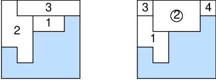
In fact, as the following theorem shows, the shortest and longest flipturn sequences may differ significantly in length.
Theorem 3.1
For infinitely many , there is an orthogonal -gon whose shortest and longest standard or extended flipturn sequences differ in length by at least .

Figure 3.2 illustrates the recursive construction of such a polygon, for all of the form . The shortest flipturn sequence for the polygon includes only diagonal flipturns and therefore has length . Another sequence, which we believe to be the longest, requires twelve flipturns to remove every vertices. Figure 3.2 illustrates this long sequence of standard flipturns; the corresponding extended flipturn sequence is essentially equivalent.
3.2 Well-chosen Flipturns
Here we develop upper and lower bounds on the length of the shortest sequence of flipturns required to convexify an orthogonal polygon. For any polygon , let denote its axis-aligned bounding rectangle.
Theorem 3.2
For all , there is an orthogonal -gon that requires standard or extended flipturns to convexify.
When is a multiple of , the polygon consists of a horizontally symmetric rectangular ‘comb’ with ‘teeth’; if is not a multiple of , we add a small rectangular notch in a bottom corner of the polygon. See Figure 3.3. (We consider a rectangle to be a comb with one tooth.) Both the teeth and the gaps between them decrease in height as they approach the middle of the polygon. Since the polygon is symmetric about its vertical bisecting line, standard and extended flipturns have exactly the same effect. The only way to eliminate the comb is through a sequence of orthogonal flipturns across the top edge of the polygon’s bounding box; each such flipturn eliminates exactly one tooth. It easily follows that every flipturn sequence for this polygon has length .

Lemma 3.3
Let be an orthogonal polygon.
- (a)
If some vertex of is not a vertex of , then has a diagonal pocket.
- (b)
If two adjacent vertices of are not vertices of , then we can perform at least two consecutive diagonal flipturns on .
(a) Suppose some corner of is not a vertex of . Some edge of lies on a line separating the missing corner from the interior of . This edge contains a diagonal lid.
(b) Without loss of generality, suppose does not contain the top left and top right vertices of . Part (a) implies that has at least two diagonal pockets. Let be the result of flipturning one of these pockets. Since the width of the flipturned pocket is less than the width of , and thus less than the width of , at least one of the upper corners of is not a vertex of . (As Figure 3.4 shows, flipturning one pocket can capture the opposite corner.) Thus, by part (a), still has at least one diagonal pocket.

This lemma is a special case of a more general result, whose proof we omit: If any vertices of are not vertices of , then we can perform at least consecutive diagonal flipturns on .
Theorem 3.4
Any orthogonal -gon can be convexified by a sequence of at most extended flipturns.
We achieve the stated upper bound by performing an orthogonal extended flipturn only when no diagonal pockets are available. By Lemma 3.3, we are forced to perform an orthogonal flipturn on a polygon if and only if all four corners of are also vertices of .
Let be a nonconvex orthogonal -gon with bounding box , and suppose has no diagonal pockets. Without loss of generality, suppose has an extended orthogonal pocket whose lid is the top edge of . This pocket obviously lies strictly between the vertical lines through and . Let be the polygon that results when this extended pocket is flipturned. The highest vertices of are vertices of the newly flipturned pocket, and thus must lie strictly between the vertical lines through and . Thus, neither of the top vertices of is a vertex of , and by Lemma 3.3, we can perform at least two consecutive diagonal flipturns on . See Figure 3.5.

In other words, any orthogonal extended flipturn can be followed by at least two diagonal flipturns. Thus, if we perform orthogonal flipturns only when no diagonal flipturn is available, any three consecutive flipturns eliminate at least four vertices.
Theorem 3.2 implies that this result is the best possible for extended flipturns. For standard flipturns, we obtain the following slightly weaker upper bound.
Theorem 3.5
Any orthogonal -gon can be convexified by a sequence of at most standard flipturns.
As in the previous theorem, we achieve the upper bound by performing orthogonal flipturns only when no diagonal flipturn is available. However, we also choose orthogonal flipturns carefully if more than one is available. Say that an orthogonal flipturn is good if it can be followed by at least two diagonal flipturns and bad otherwise. We will perform a bad orthogonal flipturn only if no good orthogonal flipturn or diagonal flipturn is available.
Let be an orthogonal polygon. Without loss of generality, consider a forced orthogonal flipturn whose lid lies on the top edge of , and let be the polygon resulting from this flipturn. See Figure 3.6(a). The lid endpoints and must lie in two different pockets of , since the flipturned pocket touches the top of . The horizontal width of the pocket must be less than the horizontal width of , so cannot have both the upper left and upper right corners of as vertices. Thus, by Lemma 3.3, any forced orthogonal flipturn can be followed first by a diagonal flipturn and then by at least one more (possibly orthogonal) flipturn. In particular, any bad flipturn can be followed by exactly one diagonal flipturn.


 (a)
(b)
(c)
(a)
(b)
(c)
Let be a polygon with no diagonal pockets or good orthogonal pockets. Consider a bad orthogonal flipturn whose lid is a subset of the top edge of , and let be the resulting polygon. Exactly one of the top corners of is a vertex of . If this is the top right corner, call pocket dexter; otherwise, call it sinister. Without loss of generality, suppose the pocket is dexter. Let be the polygon resulting from the only available diagonal flipturn, whose lid is the upper left edge of . Since must have no diagonal pockets, this flipturn moves vertex to the upper left corner of . See Figure 3.6(c).
If some pocket had a lid in , that pocket would be inverted by the diagonal flipturn on and would have a diagonal pocket, contradicting our assumption that pocket is bad. Similarly, if there is a bad pocket with lid in , it cannot be dexter. Suppose there is a sinister pocket with lid . Let be a leftmost point in pocket , and let be a rightmost point in pocket . See Figure 3.6(b). The horizontal distance from to must be equal to , and the horizontal distance from to must equal to , since both pockets are bad. But this is impossible, since . We conclude that must be the only lid on the top edge of .
Now consider the orthogonal pocket of created when pocket is flipturned. Its lid lies on the right edge of . We claim that this pocket must be good. Let be the resulting polygon when this pocket is flipturned. Since is the bottommost edge of pocket , nothing in lies above and to the right of vertex , so the upper right vertex of is not a vertex of . Since the height of pocket is less than the height of the original polygon , the bottom right vertex of is also not a vertex of . Therefore, by Lemma 3.3, can undergo at least two consecutive flipturns.
We have just shown that any forced bad flipturn is immediately followed by a diagonal flipturn, a good orthogonal flipturn, and then two diagonal flipturns. Thus, any sequence of five consecutive flipturns contains at least three diagonal flipturns, which remove at least six vertices from the polygon.
We do not believe that this upper bound is tight. In the following section, we will show that the algorithm used to prove the upper bound may not produce the shortest flipturn sequence.
3.3 Arbitrary Flipturns
In this section, we consider the length of the longest sequence of flipturns that an orthogonal polygon can undergo.
Theorem 3.6
For all , the longest standard or extended flipturn sequence for any orthogonal -gon has length at most .
We call an edge of an orthogonal polygon a bracket if both its vertices are convex or both its vertices are concave. An orthogonal -gon has at least four brackets (the highest, leftmost, lowest, and rightmost edges) and at most brackets.
We claim that flipturns do not increase the number of brackets, and that any orthogonal flipturn decreases the number of brackets by two. Let be an orthogonal polygon and let be the result of one flipturn. Any bracket of that lies completely outside the flipturned pocket is still a bracket in ; any bracket completely inside the flipturned pocket is inverted, but remains a bracket. Thus, to prove our claim, it suffices to consider just four edges, namely, the two edges adjacent to each endpoint of the lid. After symmetry considerations, there are only three cases to check for orthogonal pockets and ten cases for diagonal pockets. These cases are illustrated in Figure 3.7.

Since each orthogonal flipturn removes two brackets, and no diagonal flipturn adds brackets, there can be at most orthogonal flipturns. Since each diagonal flipturn removes two vertices, and no orthogonal flipturn adds vertices there can be at most diagonal flipturns. Thus, there can be at most flipturns altogether.
We can improve this upper bound slightly in the special case of lattice polygons—orthogonal polygons where every edge has unit length (or more generally, where every edge has integer length and denotes the perimeter instead of the number of edges).
Theorem 3.7
The longest flipturn sequence for any lattice -gon has length at most .
In any convexifying sequence, there are exactly diagonal flipturns. Every orthogonal flipturn increases the perimeter of the polygon’s bounding box by at least . The initial bounding box has perimeter at least , and the final rectangle has perimeter exactly , so the maximum number of orthogonal flipturns is at most .
How tight is the upper bound? As in the case of the shortest flipturn sequence, the answer depends on whether we consider standard or extended flipturns. Unfortunately, we do not obtain an exact answer in either case.
Theorem 3.8
For all , there is an orthogonal -gon that can undergo extended flipturns.
This follows directly from Theorem 3.2.
Theorem 3.9
For all , there is an orthogonal -gon that can undergo standard flipturns.
We construct an orthogonal -gon essentially by following the proof of Theorem 3.5. is a rectangle. is an L-shaped hexagon, which is convexified by one flipturn. is a rectangle with a rectangular orthogonal pocket in one side, which requires three flipturns to convexify. For all , consists of a rectangle with a single L-shaped pocket, where the tail of the L is an inverted and reflected copy of . See Figure 3.8. In the language of the proof of Theorem 3.5, ’s only pocket is bad—flipturning it creates one diagonal pocket and one orthogonal pocket. If we flipturn diagonal pockets whenever possible, the first five flipturns eliminate six vertices and leave a distorted . The theorem follows by induction.

To prove Theorem 3.5, we used an algorithm that always prefers diagonal flipturns to orthogonal flipturns and good orthogonal flipturns to bad orthogonal flipturns. We can use the polygon from the previous proof to show that this algorithm is not optimal, by demonstrating a shorter convexifying flipturn sequence. Figure 3.9 shows the first sixteen flipturns performed by a modified algorithm, which ignores diagonal ‘notches’ in the upper and lower right corners of the polygon. Figure 3.9(b) is distorted to reveal relevant but otherwise invisible details; the distortion does not change which flipturns we can perform at any time. These flipturns remove vertices, thereby transforming into . Thus, by induction, we can convexify in only flipturns whenever is a multiple of .

 (a)
(b)
(a)
(b)
The ignored ‘notches’ are precisely the diagonal flipturns that do not remove brackets; see Theorem 3.6. Perhaps a modified algorithm that tries to reduce the number of brackets as fast as possible, as well as the number of vertices, would improve Theorem 3.5. We leave the development of such an algorithm as an intriguing open problem.
Finally, we observe that can be convexified using exactly extended flipturns. We leave the proof as an easy exercise of the reader.
4 Flipturn Sequences for Arbitrary Polygons
In this section, we derive upper bounds for the longest flipturn sequences of arbitrary polygons, generalizing both our earlier results for orthogonal polygons and the modified flipturn results of Ahn et al. [1].
Consider an arbitrary polygon whose boundary is oriented counterclockwise. Let denote the direction of any (oriented) edge in , let be the set of all such edge directions and their edge reversals. We clearly have , where is the number of distinct edge slopes. Ahn et al. define the discrete angle at a vertex to be one more than the number of elements of inside the angle between and . The total discrete angle is the sum of the discrete angles at the vertices of .
Ahn et al. prove the following lemma [1]. (Only the first half of this lemma is stated explicitly, but their proof implies the second half as well.)
Lemma 4.1
Every non-degenerate flipturn decreases by at least two, and every degenerate flipturn leaves unchanged.
Ahn et al. also prove that in general and if is convex. Thus, Lemma 4.1 immediately implies that nondegenerate flipturns suffice to convexify any polygon. However, since no bound was previously known for the number of degenerate flipturns, this bound does not apply to degenerate polygons. To avoid this problem, Ahn et al. introduce modified flipturns, for which degeneracies do not exist. To account for degenerate flipturns under the standard definition, we study the change in the number of brackets, here denoted , as in Section 3.3.
Lemma 4.2
Every non-degenerate standard or extended flipturn increases by at most two, and every degenerate standard or extended flipturn decreases by at least two.
Let be a simple polygon and let be the result of one flipturn. As we argued in the proof of Theorem 3.6, it suffices to focus on brackets touching the endpoints of the lid. Let and denote the number of boundary brackets in and , respectively, so that .
For nondegenerate flipturns, it suffices to consider only flipturns with , since is never more than . There are three cases to consider: no boundary brackets, one outer boundary bracket, and one inner boundary bracket. For each of these, there are nine subcases, depending on whether each lid endpoint becomes a convex vertex, becomes a concave vertex, or disappears after the flipturn. These cases are illustrated in Figure 4.1.
Standard degenerate flipturns always have two outer brackets, and both lid endpoints always become concave vertices. Thus, there are only three cases to consider, depending on the number of inner brackets, exactly as in Theorem 3.6. Similar arguments apply to extended flipturns.

 , outer
 , inner
Theorem 4.3
Every -oriented polygon is convexified after any sequence of standard or extended flipturns.
We define the potential of a polygon to be its discrete angle plus half the number of brackets, that is, . For the initial polygon , we have and , so the initial potential is at most . For the final convex polygon, we have and , so the final potential is at least . By Lemmas 4.1 and 4.2, every flipturn reduces the potential by at least one. Thus, after any sequence of flipturns, the polygon must be convex.
If we set , we obtain the upper bound for arbitrary simple polygons. However, if , there can be no degenerate flipturns, so the discrete angle results from Ahn et al. apply directly, giving us the upper bound . Hence, the actual worst case arises when .
Corollary 4.4
Every simple polygon is convexified after any sequence of standard or extended flipturns.
This upper bound is almost certainly not tight. Intuitively, if large, only a few pairs of edges can have the same slope, so the maximum number of degenerate flipturns should be small.
We can improve our results in some cases using a different definition of discrete angle. Let denote the set of edge directions (without their reversals), let , and let be the maximum number of edge directions that fit in an open half-circle. The discrete angle at any vertex is at most , so for any polygon ; if is convex, then . Lemma 4.1 still holds under this new definition. Thus, we obtain the following upper bounds.
Theorem 4.5
Every simple polygon is convexified after any sequence of modified flipturns or standard or extended flipturns.
This theorem improves all earlier results whenever is significantly smaller than . For general polygons, setting gives us the same upper bound for modified flipturns. For standard or extended flipturns, however, we obtain a very slight improvement by setting .
Corollary 4.6
Every simple polygon is convexified after any sequence of standard or extended flipturns.
We close this section with some obvious open questions. Asymptotically, our bounds agree with Joss and Shannon’s conjecture [13]—any polygon can indeed be convexified by flipturns—but there is still a significant gap between our upper bounds and the lower bound construction of Biedl [3]. We, like Joss and Shannon, conjecture that the correct answer is closer to .
A more interesting open question concerns the length of shortest flipturn sequences for general polygons. The best lower bounds are those derived for orthogonal polygons in Section 3, but not subquadratic upper bounds are known. Can arbitrary polygons be convexified with only flipturns, or does some polygon require a super-linear number of flipturns to convexify?
5 Data Structures for Flipturns
In this section, we describe efficient data structures for executing a sequence of flipturns on any simple (not necessarily orthogonal) polygon. We first describe a simpler data structure that maintains an implicit description of a polygon as flipturns are performed, without worrying about how the flipturns are chosen. Then we will describe how to maintain the convex hull of as we perform flipturns, so that we can determine which flipturns are available at any time.
Lemma 5.1
After preprocessing time, we can maintain an implicit description of a simple -gon in time per flipturn, using a data structure of size .
It suffices to store only the slopes and lengths of the edges in the proper order, without explicitly storing the vertex coordinates. Any flipturn reverses a contiguous chain of edges, namely, the edges of the flipturned pocket. Our goal, therefore, is to maintain a circular list of items subject to the operation , which reverses the sublist starting with item and ending with item . For example, if the initial list is , then produces the list , after which produces .
We store the edges in the leaves of a balanced binary search tree, initially in counterclockwise order around the polygon. Rather than explicitly reversing chains of edges, we will store a reversal bit at every node , indicating whether that subtree should be considered reversed, relative to the orientation of the subtree rooted at ’s parent. Initially, all reversal bits are set to .

Our algorithm for is illustrated in Figure 5.1. Without loss of generality, we assume that appears before in the linear order stored in the tree; otherwise, we simply toggle the reversal bit at the root and call . First, we split the tree into three subtrees, containing the items to the left of , items between and , and the items to the right of . Second, we toggle the reversal bit at the root of the middle tree. Finally, we merge the three trees back together. Each split or merge can be performed using rotations (using red-black trees [15], splay trees [23], or treaps [22], for example), and we can easily propagate the reversal bits correctly at each rotation.
To maintain the convex hull of a polygon under flipturns, we use a variant of the dynamic convex hull data structure of Overmars and van Leeuwen [20], which maintains the convex hull of a dynamically changing set of points in time per insertion or deletion. Their data structure consists of a balanced binary tree that allows insertions, deletions, splits, and merges in time. The points are stored at the leaves of this tree, ordered by their -coordinates. Each node in the tree stores the convex hull of the points in its subtree; we call this the node’s subhull. Except at the root, these subhulls are not stored explicitly; rather, each node stores only the chain of edges of its subhull that are not in its parent’s subhull. Overmars and van Leeuwen show that any node’s subhull can be computed in time from its children’s subhulls, by finding the outer common tangent lines.
There are several differences between our problem and the standard dynamic convex hull problem. The most significant difference is that we need to support an operation similar to Reverse in polylogarithmic time. This requires us to store the vertices in their order of appearance around the polygon, rather than in any coordinate order. Moreover, since a linear number of vertices could be affected by a flipturn, our data structure must implicitly represent both the order and the locations of the vertices. A second significant difference lies in the structure of the subhulls. In Overmars and van Leeuwen’s data structure, the subhulls of any two siblings in the tree are separated by a known vertical line. In our case, sibling subhulls are pseudo-disks: either they have disjoint interiors, or they have nested closures, or their boundaries intersect transversely at exactly two points. Distinguishing these three cases and merging the subhulls in each case requires considerably more effort. Finally, one minor difference is that for standard flipturns, we must maintain the complete sequence of polygon vertices on the boundary of the convex hull, not just the convex hull vertices. This requires only trivial modifications, which do not deserve further mention.
Lemma 5.2
After preprocessing time, we can maintain an implicit description of the convex hull of a simple -gon in time per flipturn, using a data structure of size .
We maintain the polygon vertices in a balanced binary tree, similarly to the proof of Lemma 5.1. The coordinates of the points are represented implicitly by storing a triple at each internal node , encoding an affine transformation to be applied to all edges in the subtree of . Specifically, is a translation vector for all edges in ’s subtree if and a point of reflection if . Initially, for all nodes . The actual position of any vertex can be recovered in time by composing the transformations along the path up to the root. We can easily maintain these triples under rotations, splits, and merges, similarly to the Reverse algorithm described earlier. We omit the unenlightening details.
Each node in this tree also stores the portion of its subhull not included in its parent’s subhull. Specifically, we store the vertices of this convex chain in a secondary balanced binary tree. Instead of explicitly storing the coordinates of the vertices of this chain, however, we store only pointers to the appropriate leaves in the primary binary tree. The coordinates of any point can be recovered in time by composing the linear transformations stored on the path up from the point’s leaf.
It remains only to show that we can merge any two sibling subhulls quickly. If we can merge two sibling subhulls in time when all vertex coordinates are given explicitly, then we can update the convex hull of in time per flipturn. One logarithmic factor is the number of merges we must perform for each flipturn; the other is the cost of accessing the implicitly-stored vertex coordinates.
Let be the chain of polygon edges associated with some node in the primary binary tree, and let and be the subchains associated with the left and right children of , respectively. Since has no self-intersections, the boundaries of the convex hulls and can intersect in at most two points. If the hull boundaries do not intersect, then the hulls can be either disjoint or nested. See Figure 5.2.
 |
| (a) |
 |
| (b) |
 |
| (c) |
If and are nested, then one of them is the convex hull of . In general, deciding whether to given convex polygons are nested requires time, but the special structure of our problem allows a faster solution. We define the entrance and exit of a polygonal chain as follows. The entrance of is a pair of rays whose common basepoint is the first vertex of that is also a vertex of ; the rays contain the convex hull edges on either side of this vertex. The exit of is a similar pair of rays based at the last vertex of that is also a vertex of . See Figure 5.3.

Let be the last vertex of , and let be the first vertex of . The segment does not intersect , so if is outside the convex hull of , then must be outside the entrance of (i.e., on the opposite side of the entrance from ). More generally, if and only if lies completely inside the entrance of .33 3 If is not a vertex of , we can simplify the entrance of to a line through just one convex hull edge. While this modification simplifies our algorithm somewhat, it does not significantly improve the running time. Similarly, if and only if lies completely inside the exit of . We can test in time whether a convex polygon (represented as an array of vertices in counterclockwise order) lies inside a wedge. Thus, if we can compute the entrance and exit of any chain given those of its children, then we can test for nested sibling subhulls in time. Fortunately, this is quite easy. If both edges of defining the entrance of are also edges of , then the entrance of is just the entrance of . Otherwise, the entrance of contains one of the two outer common tangents between and .
Now suppose and are not nested. Using an algorithm of Chazelle and Dobkin [7], we can decide in time whether and intersect. If the two convex hulls have disjoint interiors, their algorithm also returns a separating line .44 4 Chazelle and Dobkin’s algorithm returns a pair of parallel separating lines, one tangent to each polygon, but this is unnecessary for our result. See also [9]. If we use as a local vertical direction, we can divide and into separate upper and lower hulls, such that one outer common tangent joins the two upper hulls and the other joins to two lower hulls. This is precisely the setup required by the algorithm of Overmars and van Leeuwen, which finds these two common tangents in time [20].
Finally, suppose the boundaries of and intersect at two points. In this case, we can find the two outer common tangent lines between them, and thus compute , in time. To find (say) the upper common tangent of and , we perform a modified binary search over the vertices of . At each step of this binary search, we find the upper tangent line to (if any) passing through a vertex in time, using a second-level binary search.
Thus, we can compute the convex hull, entrance, and exit of from the convex hulls, entrances, and exits of and in time. By our earlier argument, it follows that we can maintain the convex hull of in time per flipturn. We can build the original data structure in time by explicitly computing the convex hulls of each subchain, each in linear time.
Theorem 5.3
Given a simple -gon , a convexifying sequence of flipturns can be computed in time, where is the length of the computed sequence.
We can construct the data structures to maintain the polygon and its convex hull in time. In addition to the convex hull itself, we maintain a separate list of the lids of , which requires only trivial additions to our data structures. This allows us to choose a legal flipturn in constant time. By Lemma 5.2, we can maintain both the polygon and its convex hull in time per flipturn.
This theorem has an immediate corollary, using the results of Ahn et al. [1] and our Theorems 3.6 and 4.3.
Corollary 5.4
Given an -oriented -gon, a convexifying sequence of flipturns can be computed in time. In particular, for orthogonal polygons, a convexifying flipturn sequence can be computed in time.
For orthogonal polygons, we can modify our algorithm to find a flipturn sequence satisfying Theorem 3.5, still in time. We maintain the diagonal pockets and orthogonal lids of in separate lists. If there is a diagonal pocket, we flipturn it. Otherwise, if some edge of the bounding box contains more than one lid, we flipturn one of those pockets. If each edge of the bounding box has at most one lid, we can check whether any of these pockets is bad in time. To check one pocket, we flipturn it and count diagonal pockets; if there is only one, we flipturn that and count again. If the pocket is bad and the original polygon has any unchecked pockets, we undo the flipturn(s) and try the next pocket. Each bad flipturn requires at most seven flipturns and six anti-flipturns. The proof of Theorem 3.5 ensures that we perform at most bad flipturns, so the total number of data structure updates is at most .
It seems quite likely that our data structure can be improved. One obvious bottleneck in our algorithm is finding common tangents between intersecting convex pseudo-disks, which currently takes time. The more recent dynamic convex hull results of Chan [5] and Brodal and Jakob [4] may also be useful here. On the other hand, we are unable to prove even an lower bound, even for arbitrary polygons. What is the true complexity of computing flipturn sequences?
6 Order Doesn’t Matter
Joss and Shannon showed that any simple polygon can be transformed into a convex polygon by a sufficiently long sequence of flipturns. If we always direct polygon edges so that they form a counterclockwise cycle, then flipturns do not change the direction of any edge. Since flipturns also do not change edge lengths, the final convex shape of is the same for any convexifying flipturn sequence. We can easily compute this shape in time by sorting the edges of by their orientation. For -oriented polygons, this requires only time.
In this section, we show that the position of the final convex polygon is also independent of the flipturn sequence. To prove this result, it suffices to show that we can predict the -coordinate of the top edge of the final convex polygon’s bounding box. The position of the left edge follows from a symmetric argument, and these two edges determine the polygon’s final position.
We prove our theorem by induction on the number of flipturns.55 5 The results in this section actually hold for a wider class of pivots called generalized flipturns. A generalized flipturn rotates a chain of edges 180 degrees around the midpoint of its endpoints without introducing self-intersections. Generalized flipturns include standard, extended, and modified flipturns as special cases. Let be a non-convex polygon, let be a lid of some pocket in , and let be the midpoint of . We subdivide the plane into horizontal strips using the horizontal line through , the horizontal lines passing through every vertex of , and the reflection of across . Number the strips counting upwards from and counting downwards from . With this numbering, any strip is the reflection of strip across . In particular, strips and have the same width, which we denote . There are at most strips altogether.
These strips subdivide the exterior of into trapezoidal regions. We classify these trapezoids into several groups. If a region is unbounded, we call it an outer region; otherwise, we call it an inner region. We further classify outer regions into the infinite strips above or below (including the top and bottom halfplanes), and the semi-infinite side regions to the left or right of . We also classify inner regions as up-regions and down-regions as follows. Consider the shortest path through the exterior of starting at a point in the interior of some inner region and ending at a point in some outer region. If the first segment of this path goes up from the starting point, is an up-region; otherwise, is a down-region. We emphasize that this classification is independent of the starting point within . We show below that the total height of the up regions is precisely the distance between the top of the current polygon’s bounding box and the top of the final convex polygon’s bounding box.
For each , let denote the number of up-regions in strips and , and let be the indicator variable equal to if strip intersects and otherwise. See Figure 6.1(a).

 (a)
(b)
(a)
(b)
Let be the result of flipturning the pocket . This flipturn moves any point on the boundary of the pocket from some strip to the corresponding strip . The strips subdivide the exterior of into regions exactly as the exterior of , and we define the corresponding variables and mutatis mutandis. See Figure 6.1(b).
Our core lemma is the following.
Lemma 6.1
For all , .
Fix an index . We prove the theorem by induction on the number of inner regions in the flipturned pocket. If the pocket contains no inner regions, it must be -monotone, and we easily observe that and .
The inner regions of have a natural forest structure, defined by connecting each region to the next region encountered on a shortest path to infinity. The roots of this forest are inner regions directly adjacent to outer regions, and its leaves are inner regions adjacent to only one other region. Let be some leaf region inside pocket , let , and define and analogously to and for this new polygon. Finally, let be the result of flipturning the now-simpler pocket , let be the image of under this flipturn (so ), and define and analogously. Since has one less inner region than , the inductive hypothesis implies that .
It suffices to consider the case where lies either in strip or in strip , since otherwise we have , , , and , and so there is nothing to prove. Moreover, if is in strip , then .
Suppose is an up-region, so . Some region of is split into two regions by . If we imagine a continuous transformation from to , the trapezoid grows upward from the bottom edge of . We have four cases to consider, illustrated in the first two rows of Figure 6.2. (The last row shows the corresponding cases when is a down-region.)

- Case 1: is an up-region.
-
In this case splits into two up-regions, so . If is in strip , then is in strip , so and (but these might be either or ).
- Case 2: is a down-region.
-
In this case splits into an up-region and a down-region, so . If is in strip , then and .
- Case 3: is a side region.
-
In this case splits into an up-region and a side region, so . If is in strip , then and .
- Case 4: is a strip.
-
Since is an up-region, must touch the bottom edge of , which means that must lie above . In this case splits into two side regions, so . Since is in strip , we have but .
The lemma holds in every case. Four similar cases arise when is a down-region and . In each case, we have , , and . We omit further details.
Theorem 6.2
The final convexified position of a polygon is independent of the convexifying flipturn sequence and can be determined in time.
Let denote the vertical width of strip (and strip ). Lemma 6.1 implies that
| (1) |
Let and denote the -coordinates of the top of and , respectively, and let be the -coordinate of the lid midpoint . We easily observe that
| (2) |
Finally, define and . Combining equations (1) and (2), we obtain the identity . In other words, the total height of all the up-regions plus the maximum -coordinate of the polygon is an invariant preserved by any flipturn.
Let be the convex polygon produced by some sequence of flipturns starting from , and define and analogously to and . Obviously, has no up-regions, so . Thus, by induction on the number of flipturns, we have the identity . Since is independent of the convexifying flipturn sequence, so is the vertical position of .
We can compute in linear time by computing a horizontal trapezoidal decomposition of , using Chazelle’s algorithm [6] or its recent randomized variant by Amato, Goodrich, and Ramos [2], and then performing a depth-first search of its dual graph.
The argument for the horizontal position of is symmetric.
7 The Worst Order Is Hard to Find
Theorem 7.1
Computing the longest standard or extended flipturn sequence for a simple polygon is NP-hard.
It suffices to consider the special case of orthogonal polygons. A flipturn sequence for an orthogonal polygon has length greater than if and only if it contains an orthogonal flipturn. Thus, to prove the theorem, we only need to show the NP-hardness of the decision problem Orthogonal Flipturn: Given an orthogonal polygon, does any flipturn sequence contain an orthogonal flipturn? We prove this problem is NP-complete by a reduction from Subset Sum: Given a set of positive integers and another integer , does any subset of sum to ? The reduction algorithm is given in Figure 7.1. The algorithm constructs a polygon in linear time by walking along its edges in clockwise order, starting and ending at the top of the first step. (The algorithm assumes without loss of generality that is even.) Figure 7.2 shows an example of the reduction.
|
 (a)
(a)
 (b)
(b)
The basic structure of the polygon is a staircase, with one square step for each of the , plus one long step of height splitting the other steps in half. Just below each of the upper steps is an an inward horizontal spike; just above each of the lower steps is an outward horizontal spike; and just behind the long step is a vertical test spike of length exactly . The horizontal spikes all have length greater than , and they increase in length as they get closer to the top and bottom of the polygon.
At any point during the flipturning process, the polygon has one main pocket containing the test spike and several secondary pockets containing one or more smaller steps, each of whose heights is some . Initially, there is just one secondary pocket, of height and width . The th step (i.e., the one with height ) is exposed the th time the main pocket is flipturned. No matter which flipturns we perform before flipturning the test spike, the vertical distance between the top endpoint of the main pocket’s lid and the top edge of the polygon’s bounding box is always the sum of elements of . Specifically, if we flipturn every step whose size is an element of some subset as soon as it becomes available, then just before the test spike is flipped, is the sum of the elements of ; see Figure 7.2(b). Thus, since the test spike has length , flipturning it can create an orthogonal pocket if and only if some subset of sums to .
Note that the polygon produced by our reduction never has more than one orthogonal pocket; the longest flipturn sequence has either or flipturns. Thus, even approximating the maximum number of orthogonal flipturns is NP-hard.
Our reduction only proves that finding the longest flipturn sequence is weakly NP-hard. In particular, it says nothing about lattice polygons in their standard representation as a cycle of unit-length orthogonal segments. We conjecture that for such polygons, there is a polynomial time dynamic programming algorithm, similar to the algorithm for SubsetSum.
Finally, how hard is it to find the shortest sequence of flipturns that convexifies a given simple polygon? It seems unlikely that the question “Does every flipturn sequence have an orthogonal flipturn?” is NP-hard.
Acknowledgments
All but one of the authors thank Godfried Toussaint for organizing the Barbados workshop where most of this work was done. Thanks also to David Bremner, Ferran Hurtado, Vera Sacristán, and Mike Soss for sharing coffee, rum, and ideas.
References
- [1] H.-K. Ahn, P. Bose, J. Czyzowicz, N. Hanusse, E. Kranakis, and P. Morin. Flipping your lid. To appear in Geombinatorics X(1), 2000. http://www.scs.carleton.ca/~morin/publications/linkage/flipturn-tr.ps.
- [2] N. M. Amato, M. T. Goodrich, and E. A. Ramos. Linear-time polygon triangulation made easy via randomization. Proc. 16th Annu. ACM Sympos. Comput. Geom., pp. 201–212. 2000.
- [3] T. Biedl. Polygons needing many flipturns. Technical Report CS-2000-04, Department of Computer Science, University of Waterloo, 2000. ftp://cs-archive.uwaterloo.ca/cs-archive/CS-2000-04/.
- [4] G. S. Brodal and R. Jakob. Dynamic planar convex hull with optimal query time and update time. To appear in Proc. 7th Scandinavian Workshop on Algorithm Theory. Lect. Notes Comput. Sci., Spring-Verlag, 2000. http://www.brics.dk/~gerth/Papers/swat2000dch.ps.gz.
- [5] T. M. Chan. Dynamic planar convex hull operations in near-logarithmic amortized time. Proc. 40th Annu. IEEE Sympos. Found. Comput. Sci., pp. 92–99. 1999.
- [6] B. Chazelle. Triangulating a simple polygon in linear time. Discrete Comput. Geom. 6(5):485–524, 1991.
- [7] B. Chazelle and D. P. Dobkin. Intersection of convex objects in two and three dimensions. J. ACM 34(1):1–27, 1987.
- [8] L. E. Dubins, A. Orlitsky, J. A. Reeds, and L. A. Shepp. Self-avoiding random loops. IEEE Trans. Inform. Theory 34:1509–1516, 1988.
- [9] H. Edelsbrunner. Computing the extreme distances between two convex polygons. J. Algorithms 6:213–224, 1985.
- [10] P. Erdős. Problem number 3763. American Mathematical Monthly 42:627, 1935.
- [11] P. W. Finn, D. Halperin, L. E. Kavraki, J.-C. Latombe, R. Motwani, C. Shelton, and S. Venkatasubramanian. Geometric manipulation of flexible ligands. Applied Computational Geometry, pp. 67–78. Lecture Notes Comput. Sci. 1148, Springer-Verlag, 1996.
- [12] M. D. Frank-Kamenetskii. Unravelling DNA. Addison-Wesley, 1997.
- [13] B. Grünbaum. How to convexify a polygon. Geombinatorics 5:24–30, 1995.
- [14] B. Grünbaum and J. Zaks. Convexification of polygons by flips and by flipturns. Technical Report 6/4/98, Department of Mathematics, University of Washington, Seattle, 1998.
- [15] L. J. Guibas and R. Sedgewick. A dichromatic framework for balanced trees. Proc. 19th Annu. IEEE Sympos. Found. Comput. Sci., pp. 8–21. 1978.
- [16] N. Madras and G. Slade. The Self-Avoiding Walk. Birkhäuser, Boston, 1993.
- [17] N. Madras and A. D. Sokal. The pivot algorithm: A highly efficient Monte Carlo method for the self-avoiding walk. Journal of Statistical Physics 50:109–186, 1988.
- [18] F. M. McMillan. The Chain Straighteners. The MacMillan Press, 1979.
- [19] J. O’Rourke. Folding and unfolding in computational geometry. Discrete and Computational Geometry (Proc. JCDCG ’98), pp. 142–147. Lecture Notes Comput. Sci. 1763, Springer-Verlag, 2000.
- [20] M. H. Overmars and J. van Leeuwen. Maintenance of configurations in the plane. J. Comput. Syst. Sci. 23:166–204, 1981.
- [21] E. J. J. van Rensburg, S. G. Whittington, and N. Madras. The pivot algorithm and polygons: results on the FCC lattice. Journal of Physics A: Mathematical and General Physics 23:1589–1612, 1990.
- [22] R. Seidel and C. R. Aragon. Randomized search trees. Algorithmica 16:464–497, 1996.
- [23] D. D. Sleator and R. E. Tarjan. Self-adjusting binary search trees. J. ACM 32(3):652–686, 1985.
- [24] B. de Sz.-Nagy. Solution of problem 3763. American Mathematical Monthly 46:176–177, 1939.
- [25] G. T. Toussaint. Computational polygonal entanglement theory. Proc. VIII Encuentros de Geometría Computacional. July 7-9, 1999. http://www-cgrl.cs.mcgill.ca/~godfried/publications/castellon.ps.gz. Castellon, Spain.
- [26] G. T. Toussaint. The Erdős-Nagy theorem and its ramifications. 11th Canadian Conf. Comput. Geom., pp. 9–12. 1999. http://www.cs.ubc.ca/conferences/CCCG/elec_proc/fp19.ps.gz.