Orthogonal Least Squares Algorithm for the Approximation of a Map and its Derivatives with a RBF Network

Say $\{x(k),t(k)\}$, $k=1,2,...,N$, is the data set given by $N$ input-output data pairs, which can be organized in two column vectors ${\mathbf{x}}=[x(1)\cdots x(N)]^{T}$ and ${\mathbf{t}}=[t(1)\cdots t(N)]^{T}$. The model parameters are given in vectors ${\mathbf{m}}=[m_{1}\cdots m_{H}]^{T}$, ${\mathbf{w}}=[w_{1}\cdots w_{H}]^{T}$ and ${\mathbf{b}}=[b]$, where $H$ is the number of radial units to be used. Arranging the problem in matrix form we have:

with

where ${\mathbf{p}}_{i}=[\phi(x(1),m_{i})\dots\phi(x(N),m_{i})]^{T}$ are regressor vectors forming a set of basis vectors, ${\mathbf{e}}=[e(1)\cdots e(N)]^{T}$ is the identification error, and ${\mathbf{1}}=[1\dots 1]^{T}$ is a unit column vector of length $N$. The least squares solution of this problem satisfies the condition that

is the projection of ${\mathbf{t}}$ in a vector space spanned by the regressors. If the regressors are not independent, the contribution of each regressor to the total energy of the desired output vector is not clear. The OLS algorithm iteratively selects the best regressors from a set by applying a Gram-Schmidt orthogonalization, so that the contribution of each vector of this new orthogonal base can be determined individually among the available regressors.

The classic algorithm selects the best set of regressors from the ones available, and determines the output layer weights for the identification of the desired in-out map, but does not explicitly controls the derivative of the function. We propose to modify this procedure so to permit to specify the desired value of the function derivative in each data point. The data set will then be organized in three vectors ${\mathbf{x}}=[x(1)\cdots x(N)]^{T}$, ${\mathbf{t}}=[t(1)\cdots t(N)]^{T}$, and ${\mathbf{t}}^{(1)}=[t_{1}(1)\cdots t_{1}(N)]^{T}$, ${\mathbf{x}}$ and ${\mathbf{t}}$ being the input-output pairs and ${\mathbf{t}}^{(1)}$ being the respective derivatives. It has to be noted that the original OLS algorithm selects each radial unit from a set of units, each of which is centered on a input data point. The maximum number of units is then limited to the number of data points. When we add requirements on the derivative of the function, a further constraint to the optimization problem is added, and the number of units to be selected in order to reach the desired approximation may be higher then the number of data points. A possible choice is to augment the input vector with points where there is no data available, and to build the set of $N_{e}$ regressors on this extended vector.

The algorithm can be summarized as follows:

• •

  First step, initialization: the set of regressors for selection is obtained by centering the $N_{e}$ radial units, and the error reduction ratio (err) for each regressor vector is computed. Given the regressor vectors

  $${\mathbf{p}}_{i}=[\phi(x(1),x(i)),...,\phi(x(N),x(i))]^{T},\;\;1\leq i\leq N_{e},$$

  (12)

  and defined the first-iteration vectors

  $${\mathbf{u}}_{1,i}={\mathbf{p}}_{i},\;\;1\leq i\leq N_{e}.$$

  (13)

  The error reduction ratio associated with the $i$-th vector is given by

  $$\mbox{err}_{1,i}=({\mathbf{u}}_{1,i}^{T}{\mathbf{t}})^{2}/(({\mathbf{u}}_{1,i}^{T}{\mathbf{u}}_{1,i})({\mathbf{t}}^{T}{\mathbf{t}})).$$

  (14)

  In a similar way, the regressor vectors for the derivative of the map are computed:

  $${\mathbf{p}}_{i}^{(1)}=[\frac{\partial\phi(x(1),x(i))}{\partial x}\cdots\frac{\partial\phi(x(N),x(i))}{\partial x}]^{T},\;\;1\leq i\leq N_{e},$$

  (15)

  and the first-iteration vectors are defined:

  $${\mathbf{l}}_{1,i}={\mathbf{p}}_{i}^{(1)},\;\;1\leq i\leq N_{e}.$$

  (16)

  The error reduction ratio for the derivative is:

  	$\displaystyle\mbox{grad\_err}_{1,i}=({\mathbf{l}}_{1,i}^{T}{\mathbf{t}}^{(1)})^{2}/(({\mathbf{l}}_{1,i}^{T}{\mathbf{l}}_{1,i})({{\mathbf{t}}^{(1)}}^{T}{\mathbf{t}}^{(1)})),$		(17)
  	$\displaystyle 1\leq i\leq N_{e}.$

  The $\mbox{ err}_{1,i}$ and $\mbox{ grad\_err}_{1,i}$ represent the error reduction ratios caused respectively by ${\mathbf{u}}_{1,i}$ and ${\mathbf{l}}_{1,i}$, and the total error reduction ratio can be computed by

  $$\mbox{ tot\_err}_{1,i}=\lambda\mbox{ err}_{1,i}+(1-\lambda)\mbox{ grad\_err}_{1,i},$$

  (18)

  where $\lambda$ weights the importance of the map against its derivative. The index $i_{1}$ is then found, so that:

  $$\mbox{tot\_err}_{1,i_{1}}=\max_{i}\{\mbox{tot\_err}_{1,i},\;\;1\leq i\leq N_{e}\}.$$

  (19)

  The regressor ${\mathbf{p}}_{i_{1}}$ giving the largest error reduction ratio is selected and removed from the set of available regressors. The corresponding center is added to the set of selected centers:

  $${\mathbf{u}}_{1}={\mathbf{u}}_{1,i_{1}}={\mathbf{p}}_{i_{1}};$$

  (20)

  $${\mathbf{l}}_{1}={\mathbf{l}}_{1,i_{1}}={\mathbf{p}}_{i_{1}}^{(1)};$$

  (21)

  $$m_{1}=x(i_{1}).$$

  (22)

• •

  $h$-th iteration, for $h=1,...,H$ and $H\leq N_{e}$: the regressors selected in the previous steps, having indexes $i_{1},...,i_{h-1}$, have been removed from the set of available regressors. Before computing the error reduction ratio for each regressor still available, the orthogonalization step is performed which makes each regressor orthogonal with respect to those already selected:

  $${\mathbf{u}}_{h,i}={\mathbf{p}}_{i}-\sum_{j=1}^{h-1}({\mathbf{u}}_{j}^{T}{\mathbf{p}}_{i})/({\mathbf{u}}_{j}^{T}{\mathbf{u}}_{j}){\mathbf{u}}_{j},\;\;i\neq i_{1},i_{2},...,i_{h-1};$$

  (23)

  $${\mathbf{l}}_{h,i}={\mathbf{p}}_{i}^{(1)}-\sum_{j=1}^{h-1}({\mathbf{l}}_{j}^{T}{\mathbf{p}}_{i}^{(1)})/({\mathbf{l}}_{j}^{T}{\mathbf{l}}_{j}){\mathbf{l}}_{j},\;\;i\neq i_{1},i_{2},...,i_{h-1};$$

  (24)

  $$\mbox{err}_{h,i}=({\mathbf{u}}_{h,i}^{T}{\mathbf{t}})^{2}/(({\mathbf{u}}_{h,i}^{T}{\mathbf{u}}_{h,i})({\mathbf{t}}^{T}{\mathbf{t}})),\;\;i\neq i_{1},i_{2},...,i_{h-1};$$

  (25)

  	$\displaystyle\mbox{ grad\_err}_{h,i}=({\mathbf{l}}_{h,i}^{T}{\mathbf{t}}^{(1)})^{2}/(({\mathbf{l}}_{h,i}^{T}{\mathbf{l}}_{h,i}){({\mathbf{t}}^{(1)}}^{T}{\mathbf{t}}^{(1)})),$		(26)
  	$\displaystyle i\neq i_{1},i_{2},...,i_{h-1};$

  	$\displaystyle\mbox{ tot\_err}_{h,i}=\lambda\mbox{err}_{h,i}+(1-\lambda)\mbox{ grad\_err}_{h,i},$		(27)
  	$\displaystyle i\neq i_{1},i_{2},...,i_{h-1}.$

  As before, the regressor with maximum error reduction ratio is selected and removed from the list of availability, and its center is added to the set of selected centers:

  $$\mbox{ tot\_err}_{h,i_{h}}=\max_{i}\{\mbox{ tot\_err}_{h,i},\;\;i\neq i_{1},i_{2},...,i_{h-1}\}$$

  (28)

  $${\mathbf{u}}_{h}={\mathbf{u}}_{h,i_{h}};$$

  (29)

  $${\mathbf{l}}_{h}={\mathbf{l}}_{h,i_{h}};$$

  (30)

  $$m_{h}=x(i_{h}).$$

  (31)

• •

  Final step, computation of output layer weights : once the $H$ radial units have been positioned, the remaining ${\mathbf{w}}$ and ${\mathbf{b}}$ parameters can be found with a Moore-Penrose matrix inversion: let us call ${\mathbf{P}}_{H}=[{\mathbf{u}}_{1}{\mathbf{u}}_{2}\cdots{\mathbf{u}}_{H}]$ and ${\mathbf{P}}_{H}^{(1)}=[{\mathbf{l}}_{1}{\mathbf{l}}_{2}\cdots{\mathbf{l}}_{H}]$ the two sets of selected regressors, and let ${\mathbf{1}}=[1\dots 1]^{T}$ and ${\mathbf{0}}=[0\dots 0]^{T}$ be two column vectors of length $N$. Then we have

  $$\left[\begin{array}[]{c}{\mathbf{t}}\\ {\mathbf{t}}^{(1)}\end{array}\right]=\left[\begin{array}[]{cc}{\mathbf{P}}_{H}&{\mathbf{1}}\\ {\mathbf{P}}_{H}^{(1)}&{\mathbf{0}}\end{array}\right]\left[\begin{array}[]{c}{\mathbf{w}}\\ {b}\end{array}\right]+{\mathbf{e}}_{H}$$

  (32)

  whose solution is

  $$\left[\begin{array}[]{c}\mathbf{w}\\ {b}\end{array}\right]=\left(\left[\begin{array}[]{cc}{\mathbf{P}}_{H}&{\mathbf{1}}\\ {\mathbf{P}}_{H}^{(1)}&{\mathbf{0}}\end{array}\right]\right)^{+}\left[\begin{array}[]{c}\mathbf{t}\\ {\mathbf{t}^{(1)}}\end{array}\right].$$

  (33)

Usually, it is convenient to stop the procedure before the maximum number of radial units has been reached, as soon as the identification error is considered to be acceptable. To this purpose, one can use equation (33) at iteration $h$ to compute the identification error ${\mathbf{e}}_{h}$ in (32) ¹¹ 1 Note that in this case the length of vector ${\mathbf{w}}$ and the number of columns of matrices ${\mathbf{P}}$ in equation (33) is $h$ instead of $H$.

Let us consider, as an example, the fitting of a step-like data set, where the derivative is arbitrarily constrained. The data set is shown in Fig. 1, along with the result of the parametric identification routine. It can be seen how an unlikely derivative was chosen in the critical zone to highlight the properties of the model. Fig. 2 shows the interpolating properties of the resulting RBF Network when computed on an input interval which is denser than the original input data set.

The single loop feedback circuit depicted in Fig. 3 is an example of autonomous non-linear system capable of different dynamical behaviors, such as decaying oscillation, stable periodic motion (including constant), and chaos.

We will consider the case where $G(z)$ is made of two cascaded linear elements, i.e. a delay line $D_{L}(z)$ of given length $L$, and a low-pass filter $H(z)$. The function $f$ is assumed to be a three-fixed points smooth function crossing the origin with slope $S_{1}$, and having slopes $S_{2}$ and $S_{3}=S_{2}$ in the other two points (see Fig. 4-a). The topology of fig. 3 is of particular interest in the field of sound synthesis, for the physically inspired modeling of musical instruments with sustained sound [13, 14], and has been object of investigation by the authors for the construction of generalized musical tone generators [15]. The length of the delay line, which can be seen as the medium where sound propagates (such as a flute pipe or a violin string), is inversely proportional to the pitch of the signal generated, and represents an example of sound control parameter with a clear physical meaning. The shape of the non-linear map and its fixed-point derivatives are recognized to be responsible for the stability of periodic motion, for the spectral content of the signal, and for the time-constant of transient extinction. We don’t care here about the shape of the map, and we focus on the fixed points and their derivatives. The condition for instability of the fixed point in the origin, and thus the condition for the system to oscillate, can be stated in terms of the Nyquist plot of the open loop transfer function $G(z)=D_{L}(z)H(z)$. Say that $-q+j0$ denotes the leftmost intersection point of the Nyquist plot of $G(z)$ with the real axis. In order to let the system oscillate, a necessary condition for $S_{1}$ is $S_{1}<-1/q$ [14]. A different role is assumed for the slope $S_{2}$, which is responsible for limiting the growth of the system state. To this purpose, a slope $S_{2}>-1$ is needed at some distance from the origin, in correspondence of the other two fixed points.

As a practical example, a low-pass filter $H(z)=0.4+0.3z^{-1}$ and a delay length $L~=~100\;\mbox{samples}$ are considered. The Nyquist plot of $G(z)$ has the smallest intersection point with the real axis in $-0.7+j0$ which gives a maximum slope of -1.4286 over which the oscillation will not occur. The length $L=100$ for the delay line gives a period length $T_{p}=200$, which corresponds to a pitch of $110.25$ Hz at a sample rate of $22050$ Hz. In Fig. 4, the time evolution of the system is shown for a map $f$ with fixed points $(0,0)$, $(-100,100)$, $(100,-100)$, for different values of the slope $S_{1}$, and for a random initial state in the range $[-0.1,0.1]$. It can be seen that the slope $S_{1}$ can be used to drive the system to a periodic steady state and to control the transient velocity.

The example shown is a particular case of the more general Hopf bifurcation theorem [16] in its frequency domain formulation. It is interesting to point out that the single loop feedback systems exemplified in [16] are discretized versions of simple $RLC$ electrical circuits, with at least a non-linear component (e.g., a tunnel diode). The result is a feedback scheme as the one in Fig. 3, where $G(z)$ is a second-order $IIR$ transfer function, and no delay lines are considered in the loop. In these circuits, a stable almost sinusoidal oscillation is reached, whose frequency and amplitude are functions of the second and third derivatives of the non-linear map $f$, evaluated in the equilibrium point (i.e., dc operating point), which is solution of the equation $G(0)f(y)-y=0$.

Still referring to the closed loop feedback system of Fig. 3, we are now interested in the stabilization of a given periodic motion. With respect to the case of Section IV-A, we’re facing the dual situation, where we ignore the transient part of the process and we’re interested in the shape of the period of the resulting time series.

Let us call ${\mathbf{y}}=[y_{1},y_{2},\dots,y_{T_{p}}]^{T}$ the desired period and assume that the length of the period is even, i.e. $T_{p}=2L$. For simplicity we consider the case that the filter $H(z)$ is not present, thus the linear system $G(z)$ is just a delay line $D_{L}(z)$, which has to be of length $L$, as seen in the previous example. The construction of the non-linear map able to produce the desired periodic waveform is straightforward, and relies on the training set $\mathcal{Y}$ computed using the data points:

where

and

In Fig. 5, the computation of the training set from the desired output process is illustrated, as well as the approximation of the unknown function given by the proposed algorithm.

If the system state is initialized with a half-period, i.e. is ${\mathbf{x}_{0}}=[y_{1},y_{2},\dots,y_{L}]^{T}$, the non-linear map iteratively computes the other half. The stability and robustness with respect to additive noise is granted by the derivative of the map, which has to be less then one in magnitude. Fig. 6 shows the time evolution of the system whose non-linear map data point derivatives are constrained to a magnitude of $0.3$, and whose evolution is temporarily disturbed with additive noise, with a SNR of $46$ dB.

One might be curious about the possibility of reaching a desired stable periodic motion from a quasi-zero random state, controlling the slope in the origin as in the previous example. Despite the fact that the solution appears to be in the combined use of the skills given in the previous examples, whether such control would be possible or not with a time-invariant 1-in 1-out non-linear map, seems to be a non-trivial problem.

If the filter $H(z)$ is not omitted in $G(z)$, the control of stability of the single loop feedback system of Fig. 3 can be conveniently approached by studying the Jacobian matrix $J$ of the map $F$ which describes the state transition ${\mathbf{x}}(n+1)=F({\mathbf{x}}(n))$ at every successive time step, $\mathbf{x}$ being the global state of the system. Let the linear element $G(z)$ be, as before, the cascade of a delay line $D_{L}(z)=z^{-L}$ of length $L$ and a low-pass filter $H(z)$. We are interested in leading the system to a stable periodic motion. In a steady state situation, the state ${\mathbf{x}}_{L}=[x_{1},x_{2},\dots,x_{L}]^{T}$ of the delay line undergoes a linear distortion due to the filtering stage. This is represented by the $L$-point circular discrete-time convolution [17]

To restore the original state of the delay line the non-linear map $f$ can be shaped on the base of a training set given by equation (48), with

and

In general, the geometric locus given by the training set ${\mathcal{Y}}$ will not necessarily be a curve of dimension 1, and the map will need to be unfolded in a higher dimensional space. We consider here the case where a one-dimensional map is sufficient to our purposes. If $H(z)$ is a first order FIR filter with coefficients $b_{1}$ and $b_{2}$, the system can be given in its state space form as

where ${\mathbf{x}}(n)=[x_{0}(n)x_{1}(n)\cdots x_{L}(n)]^{T}$ is the global state of the system at time $n$.

The Jacobian matrix of the state transition map, evaluated in $\hat{{\mathbf{x}}}=[\hat{x}_{0}\hat{x}_{1}\cdots\hat{x}_{L}]^{T}$, is given by

where

A periodic orbit $[\hat{{\mathbf{x}}}(n)\cdots\hat{{\mathbf{x}}}(n+2L-1)]$ of period $2L$ is asymptotically stable if the Jacobian ${\mathbf{J}}$ has eigenvalues of magnitude less than one for each point of the periodic orbit. The eigenvalues of ${\mathbf{J}}$ are the roots of the polynomial $z^{L+1}-b_{1}dz-b_{2}d$, and are plotted in Fig. 7 for $L=3$, and for different values of $d$. The lower and the upper figures refer to two different low-pass filters $H(z)$.

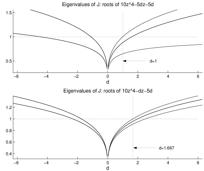
Let us focus the attention on the case where $L=3$ and $H(z)$ has coefficients $b_{1}=0.1$ and $b_{2}=0.5$. From Fig. 7 it can be seen that ${\mathbf{J}}$ has eigenvalues $|\lambda|<1$ if $|d|<1.667$. Thus, in order to have a stable and noise-robust periodic solution, the magnitude of the derivative of the map in each point of the training data must not exceed $1.667$.

Usually, a perturbation to the closed loop system is modeled with random noise added to the loop at a given point. However, it can be of some interest to vary the parameters of the linear components in the loop such as, for example, the low-pass filter $H(z)$. This can be useful to control the spectral content of the resulting time series. The stability of the whole system is thus investigated by applying, for a short time window, a perturbation to the filter coefficients $b_{1}$ and $b_{2}$. Fig. 8 shows the reaction of the system to a random perturbation, with an upper bound in magnitude of $0.02$, occurring at sample time $44$ and ending at sample time $48$. It can be seen that the perturbation will be persistent for values of $|d|$ higher than $1.667$ (upper figure), and that it will be rejected for $|d|<1.667$ in a time that is shorter the lower we choose $|d|$ (middle and lower figures).

References

- [1] S. Chen, C. F. N Cowan, and P. M. Grant, “Orthogonal least squares learning algorithm for radial basis functions networks,” IEEE Trans. on Neural Networks, vol. 2, no. 2, pp. 302–309, March 1991.
- [2] S. Haykin, Neural Networks. A Comprehensive Foundation, Macmillan, New York, 1994.
- [3] S. Haykin and J. Principe, “Making sense of a complex world,” IEEE Signal Processing Mag., vol. 15, no. 3, pp. 66–81, May 1998.
- [4] S. Chen and S. A. Billings, “Neural networks for nonlinear dynamic system modelling and identification,” Int. J. of Control, vol. 56, no. 2, pp. 319–346, 1992.
- [5] G. P. Liu, V. Kadirkamanathan, and S. A. Billings, “Variable neural networks for adaptive control of nonlinear systems,” IEEE Trans. on Systems, Man, and Cybernetics-C, vol. 29, no. 1, pp. 34–43, February 1999.
- [6] R. Langari, L. Wang, and J. Yen, “Radial basis function networks, regression weights, and the expectation-maximization algorithm,” IEEE Trans. on Systems, Man, and Cybernetics-A, vol. 27, no. 5, pp. 613–623, September 1997.
- [7] P. Yee and S. Haykin, “A dynamic regularized radial basis function network for nonlinear, nonstationary time series prediction,” IEEE Trans. on Signal Processing, vol. 47, no. 9, pp. 2503–2521, September 1999.
- [8] M. Casdagli, “Nonlinear prediction of chaotic time series,” Physica D, vol. 35, pp. 335–356, 1989.
- [9] F. J. Romeiras, C. Grebogy, E. Ott, and W. P. Dayawansa, “Controlling chaotic dyanamical systems,” Physica D, vol. 58, pp. 156–192, 1992.
- [10] J. T. Connor, R. D. Martin, and L. E. Atlas, “Recurrent neural networks and robust time series prediction,” IEEE Trans. on Neural Networks, vol. 5, no. 2, pp. 240–254, March 1994.
- [11] K. Hornik, M. Stinchcombe, and H. White, “Universal approximation of an unknown mapping and its derivatives using multilayer feedforward networks,” Neural Networks, vol. 3, pp. 551–560, 1990.
- [12] P. Cardaliaguet and G. Euvrard, “Approximation of a function and its derivatives with a neural network,” Neural Networks, vol. 5, pp. 207–220, 1992.
- [13] M. E. McIntyre, R. T. Schumacher, and J. Woodhouse, “On the oscillation of musical instruments,” J. of Acoustical Soc. of America, vol. 74, no. 5, pp. 1325–1345, 1983.
- [14] X. Rodet, “Models of musical instruments from Chua’s circuit with time delay,” IEEE Trans. on Circuits and Systems, vol. 40, no. 10, pp. 696–701, 1993.
- [15] C. Drioli and D. Rocchesso, “Learning pseudo-physical models for sound synthesis and transformation,” Proc. of IEEE Int. Conf. on Systems, Man, and Cybernetics, pp. 1085–1090, October 1998.
- [16] L. O. Chua, “Nonlinear circuits,” IEEE Trans. on Circuits and Systems, vol. CAS-31, no. 1, pp. 69–87, January 1984.
- [17] A. V. Oppenheim and R. W. Schafer, Discrete-Time Signal Processing, Prentice-Hall, Inc., Englewood Cliffs, NJ, 1989.