BDD–based Reasoning in the Fluent Calculus — First Results
Abstract
The paper reports on first preliminary results and insights gained in a project aiming at implementing the fluent calculus using methods and techniques based on binary decision diagrams. After reporting on an initial experiment showing promising results we discuss our findings concerning various techniques and heuristics used to speed up the reasoning process.
Keywords: Reasoning about Actions, Fluent Calculus, Planning, Binary Decision Diagrams.
Introduction
In recent years we have seen highly advanced and novel implementations of propositional calculi and systems like, for example, GSat and its variants [1992], Smodels [1997] or DLV [1998], to mention just a few. The implementations were applied to many interesting fields in Intellectics like, for example, planning or non–monotonic reasoning. On the other hand, few results are reported so far on applying another propositional method in these fields, viz., model checking using binary decision diagrams (BDDs), with Cimatti et. al (?; ?; ?) and [1999a] being an exception. This comes to a surprise because model checking using binary decision diagrams has significantly improved the performance of algorithms and enabled the solution of new classes of problems in related areas like formal verification and logic synthesis (see e.g. [1992, 1994]). Can we adopt the technology developed for model checking of finite state machines using binary decision diagrams for the solution of planning problems and, more generally, problems occurring in reasoning about situations, actions and causality? Can we enrich these techniques by exploiting the experiences made in the state of the art implementations of propositional logic calculi and systems mentioned at the beginning of this paragraph?
In order to answer these and related questions a sound and complete mapping from (a fragment of) the fluent calculus [1990, 1998a] to propositional logic is specified in [1999] such that the entailment problem in the fluent calculus can be solved by finding models for the corresponding propositional logic formula. The propositional logic formulae are represented by reduced and ordered binary decision diagrams and techniques from model checking are applied to search for models. Our mapping relies on three properties of the considered fragment of the fluent calculus:
- •
The set of states is characterized by a finite set of propositional fluents, i.e., a set of propositional variables, which can take values out of .
- •
The actions are deterministic and their preconditions as well as effects depend only on the state they are executed in.
- •
The goal of the planning problem is a property which depends solely on the reached state.
Here we report on initial results, findings and insights gained with the BDD–based implementation of the fluent calculus. After briefly discussing the fluent calculus and the implementation using an example from the so–called Gripper–class, we concentrate on two heuristics and techniques which can be applied to speed up the solution of the planning problem. In particular, we discuss some results on variable ordering and partitioning of the transition relation.
Gripper Planning Problems
In a contest held at AIPS98, planners had to solve various problems, among which were the problems of the so–called Gripper class:
A robot equipped with two grippers and can move between two rooms and . Initially the robot is in room together with a number of balls . The task is to transport these balls into room .
We will specify Gripper class problems in the fluent calculus in a moment. Before doing so, however, some notational conventions are helpful. Words starting with an upper letter denote constants, whereas words starting with a lower letter denote predicate symbols, non–nullary function symbols and variables. Additionally we assume that each variable denotes an action, a situation, a fluent and a state (i.e. are variables of the corresponding sorts in the fluent calculus, see [1998a, 1999]). All symbols may be indexed.
In the fluent calculus situations are denoted by standing for the initial situation, and by use of the function , denoting the situation after execution of an action in an situation . States are denoted by combining the fluents, which hold in the state, with the associative and commutative binary operation symbol , effectively representing multisets of fluents. In the case of propositional fluents, as considered in this paper, the states contain each fluent at most once. represents the empty state. Thus, fulfills the properties:11 1 Free variables in formulae are assumed universally quantified, unless otherwise stated.
| (AC1) |
A normal form to write ground state terms are the so–called constructor state terms of the form , where the ’s are pairwise distinct.
denotes the state holding in a situation . We also make frequently use of the abbreviation
The initial state of a reasoning problem in the fluent calculus is specified by an axiom of the form
| (1) |
relating the initial situation to a state represented as an constructor state term. If an equation like (1) is given, then denotes the equation . Turning to the example, the initial state of a Gripper class problem is specified by
where is instantiated to some number.
The fluent states that ball is at room , states that gripper is free and states that the robot is at room . 22 2 Formally, , , denote variables of new sorts ball, room and gripper.
There are three actions in the Gripper class:
- •
the robot may move from one room to the other.
- •
the robot may pick up a ball if it is in the same room as the ball and one of its grippers is empty.
- •
the robot may drop a ball if it is carrying one.
These actions are specified by means of state update axioms, which relate a state and the state after executing an action . The general form for state update axioms is as follows:
where are positive Effects of , i.e. the fluents which did not hold before and will hold after executing the action, negative Effects and is the condition under which the action has exactly these Effects. For technical reasons we include an action noop which leaves the state unchanged.
The states, which may occur in a planning problem, are constrained the following axiom, which states, that fluents cannot occur twice in a state:
The complete fluent calculus axiomatization of a planning problem consists of the axioms mentioned above, as well as some additional axioms, whose discussion is out of the scope of this paper, namely a set of equational axioms containing (AC1), which define the semantics of , as well as a set of unique name assumptions for the sort fluent. Please refer to the given literature for a detailed discussion.
Reasoning problems themselves are specified as entailment problems in the fluent calculus. For the Gripper class we obtain the entailment problem
In general, reasoning about planning problems in the fluent calculus amounts to solving an entailment problem of the form
where is a goal formula with as the only free variable. Such problems have a solution if we find a substitution for such that
| (2) | |||
| and | |||
| (3) | |||
It is sufficient to restrict our search to substitutions which actually denote states of our reasoning problem, i.e., substitutions which contain solely bindings of variables of sort state to constructor state terms. Such substitutions are called constructor state substitutions. In the sequel, will always denote a constructor state substitution.
The main idea of our algorithm presented in [1999, 2000] is to calculate successively a sequence of sets of solutions to (2) which correspond to the sets of states reached after executing actions starting in the initial state, until a state is found which is a goal state, i.e. the corresponding substitution fulfills (3), or, if no new states are reached, in which case there is no plan. The implementation of this algorithm is done by representing these sets as well as the relation between them by means of binary decision diagrams (BDDs).
Binary Decision Diagrams
The idea of BDDs is similar to decision trees: a Boolean function is represented as a rooted acyclic directed graph. The difference to decision trees is that there is a fixed order of the occurrences of variables in each branch of the diagram, and that isomorphic substructures of the diagram are represented only once.33 3 Thus, the BDD is ordered and reduced, also called ROBDD. These properties are so useful that they are required in almost all BDD applications, so many authors include these properties into the definition of BDDs. This can lead to exponential savings in space in comparison to representations like decision trees or disjunctive or conjunctive normal form.
We will introduce BDDs via an example. A formal treatment of BDDs is out of the scope of this paper and we refer the interested reader to the literature (see e.g. [1986, 1994, 1992]).
![[Uncaptioned image]](0003047v1/aborcdbdd.png)
Consider the propositional logic formula . Using the variable ordering a BDD representation of this formula is given in the figure to the right. For a given valuation of the propositional variables and the value of the Boolean function represented by the BDD is obtained by traversing the diagram starting from the root and taking at each node the edge labeled with the value of the variable occurring in the node.
The label of the terminal node defines the value of the function under the current valuation. For example leads to a node labeled , i.e., the value of the formula is wrt this valuation.
Bryant has shown in [1986] that, given a fixed variable order, every Boolean function is represented by exactly one BDD. Moreover, propositional satisfiability, validity and equivalence problems are decidable over BDDs in linear or constant time. Of course, the complexity of the mentioned problems does not go away: the effort has been moved to the construction of the BDDs. But as Bryant has shown as well, there are efficient algorithms for logical operations, substitutions, restrictions etc. on BDDs, whose cost is in most cases proportional to the size of its operands. BDDs may be used as a theorem prover, i.e., by construction of a BDD corresponding to a logical formula, and check the BDD for interesting properties, but more often they are used as an implementation tool for algorithms which are semantically based on Boolean functions or, equivalently, propositional formulae, or, via the characteristic functions, sets. In the implementation these formulae or sets are always represented as BDDs. The use of BDDs in this paper follows this spirit.
The Algorithm
The algorithm for solving entailment problems in the fluent calculus follows in spirit the algorithm to find reachable states in finite state systems as presented e.g. in [1994]. As mentioned, the aim is to find the sets of solutions for (2) representing states which can be reached from the initial state after the execution of actions. The first crucial question to tackle is how to represent these sets using BDDs.
Each solution to (2) is a constructor state substitution with a term of the form , where the ’s are pairwise distinct. On first glance it seems impossible to represent substitutions by finite BDDs because there are infinitely many terms. Fortunately, however, if there are only finitely many fluents then there are also only finitely many terms such that satisfies (2) due to . Furthermore, because is an AC1–symbol in the fluent calculus we do not have to distinguish between terms which are equivalent under the AC1 equational theory. In other words, a term occurring in the codomain of a constructor state substitution is uniquely characterized by the set of fluents occurring in .
This observation opens a possibility for encoding sets of solutions for the entailment problem in the fluent calculus into a BDD: for each of the finitely many fluents which may occur in the binding for a variable in a constructor state substitution we introduce a propositional variable . A constructor state substitution is represented by a valuation for these variables such that is mapped to by iff occurs in . 44 4 A substitution containing more than one binding is represented similarly: for each variable in the domain of the substitution we introduce a separate set of propositional variables which encodes the binding of that variable. Hence, a set of constructor state substitutions is represented by a set of valuations. The set of valuations itself is represented by a propositional formula such that the set of models for is the set of valuations. Finally, is represented by a BDD. For example, if the alphabet underlying the fluent calculus contains precisely the fluent symbols and , then a substitution is represented by a valuation as follows:
and set is represented by the formula .
Before we return to the application of BDDs, let us first consider the process of calculating the sequence . can be immediately derived from . But how can we compute given and ? In order to answer this question we define
| (4) |
for each state update axiom of the form
Furthermore, for the set we define
| (5) |
This definition is motivated by the following result, whose proof can again be found in [1999]
Lemma 1.
Let and be two constructor state terms and . Then,
Applying this lemma we are able to characterize our sequence without implicitly referring to by the use of state:
| (6) |
where
| (7) | ||||
| (8) |
The crucial point of our application of methods and techniques based on BDDs to reasoning in the fluent calculus is the following: We could identify a class F of formulae over the alphabet underlying the fluent calculus and a transformation mapping each to a propositional logic formula such that (i) the class is expressive enough to represent interesting entailment problems wrt the fluent calculus (namely, it contains the formulae like defined in (7) and (8)) and (ii) the following result holds:
Lemma 2.
Let and a constructor state substitution such that does not contain any free variables. Then,
The axiom set contains the basic equational theory behind the fluent calculus fragment used in this paper, and describes the semantics of . The precise definition of F and as well as the proof of this lemma is beyond the scope of this paper and we refer the interested reader to [1999] or [2000] for the details. The class F is subset of all fluent calculus formulae consisting of restricted forms of equations of type without use of function symbol state, as well as boolean combinations of these and a restricted form of existential quantification over state variables.
Applying the translation to the sequence of formulae we obtain a procedure for calculating the sequence as follows. Let be the finite set of fluents in the alphabet underlying the fluent calculus. Furthermore, let denote a propositional logic formula built over the propositional variables . The sequence of propositional logic formulae corresponding to is defined by
| (9) | |||||
| (10) |
where is the vector of propositional variables used to encode and is an abbreviation for with
The propositional formulae are exactly the translations of the fluent calculus formulae by means of , and thus, because of lemma 2, representations of the sequence of sets .
From (9) and (10) the so called forward pass of our planning algorithm for computing the sequence can be derived:
- 1.
Define , in form of the BDD–representation of , such that it contains only the initial state of the reasoning problem.
- 2.
Recursively calculate , in form of the BDD-representation of , based on and , until either overlaps with the set of goal states, in which case the reasoning problem is successfully solved or no new states are generated, in which case the reasoning problem is unsolvable.
The algorithm is illustrated in Fig. 1. Starting from the initial state all reachable states are generated. The algorithm terminates as soon as this set of states overlaps with the set of goal states or can no longer be expanded. The inclusion of a special noop Action, which leaves the state unchanged, ensures that the sets consecutively grow larger such that we know that all states have been visited iff . Alternatively to the inclusion of a noop Action, one can check for cycles in the sequence of sets and whether the sets become empty.55 5 When applying frontier simplification, as discussed later, the set becomes empty when all states have been considered. In either case the algorithm is guaranteed to terminate after at most steps, where denotes the number of fluents, since the number of reachable states is at most and thus the length of the shortest plan can be at most (such that every state is visited once).
If the forward pass terminates successfully, then in a second step a shortest plan is constructed. This is done by choosing a state from and searching for a chain of states through which this state can be reached from the initial state. This is done by iterating backwards through the sets generated by the forward pass algorithm. Because this second step is a computationally (relatively) inexpensive part, we refer the interested reader to [1999], where also the soundness and completeness of the combined algorithm is established.
Optimizations
The planning approach described above is an implicit66 6 It is called implicit because the calculated sets of states are never explicitly enumerated, but represented as a whole by a BDD, whose size depends more on the structure of the set, than on its actual size. breadth first search. In each single step we search the whole breadth of the search tree in depth . The sets can get quite complex and their BDDs quite large. Even more so, the size of the BDD for , which describes the relation between the , can quickly become too large to be handled in a graceful manner. Our approach shares this problem with related model checking algorithms. Thus, a number of techniques were invented to limit a potential explosion in its size. In the sequel some of these techniques and their effects are discussed.
Variable Order
It is well known that the variable order used in a BDD has a large influence on the size of the BDD. Unfortunately it is still a difficult problem to find even an near optimal variable order.77 7 The problem to find the optimal variable order is NP-complete. Often, a good and acceptable variable order is found by empiric knowledge and experimentation. A general rule is to group variables viz. fluents, which directly influence each other, together. In particular, the variables and occurring in should be ordered next to each other order. But how should these variable groups be arranged? An ordering we call sort ordering led to good results in several reasoning problems (see Tab. 1). The idea underlying the sort ordering is to group fluents by their arguments. For example, in the Gripper class the fluents should be grouped together, because they share the argument . Remember that the fluent calculus is sorted. The sort ordering works as follows. First one considers the argument of each fluent which belongs to the largest sort and sorts the fluents according to this argument. The remaining ambiguities are resolved by considering the argument of the second largest sort and so forth as well as the leading function symbol. For some domains Tab. 1 shows some almost dramatic improvements in the size of the BDDs for sort ordering if compared to a simple lexical ordering. The latter results in grouping fluents with the same leading function symbol together. For some domains, however, there is little or no improvement; this is usually the case when there are no large sets of objects as parameters for fluents.
| Problem | Gripper | Blocksworld | get–paid |
|---|---|---|---|
| (20 Balls) | (8 Blocks) | ||
| lexical | 217409 | 206995 | 25633 |
| sort ordered | 3087 | 23373 | 38367 |
Partitioning of the Transition Relation
The maximal size of a BDD is exponential in the number of propositional variables it contains. Thus, the BDD representing , which contains twice as many propositional variables as the BDDs representing the , is prone to get very large. A way to reduce this problem is to divide the disjunction into several parts , which correspond to subsets of the state update actions.
Fig. 2 illustrates the partitioning of the transition relation.
The positive effect of the partitioning is that the actions in each subset effect only a subset of all fluents. Because the maximal size of a BDD is exponential in the number of propositional variables, the sum of the sizes of the BDDs corresponding to the partition may be significantly smaller than the size of the original BDD.
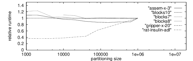
In our implementation the number of partitions is adaptive: first the BDDs for every single action are constructed, then they are combined until a parameter “partition treshold” is exceeded. In the experiments, partitioning led to a reduction of needed memory in most of the tested problems as shown in Fig. 4 at the end of the paper.
On the other hand, a reduction in memory size does not necessarily lead to a reduction in calculation time as the results depicted in Fig. 3 indicate. According to equation (11) the various parts of the partitioned transition relation have to be put together, and this takes time. Nevertheless splitting can be useful even if the computation time increases, because of the reduction of the needed memory to store the BDDs. For example in the case of mprime–x–1 the problem was not manageable under our memory constraints without partitioning the transition relation.
The idea to partition BDDs can also be applied to the BDDs representing . We have not yet explored this idea, because in our test problems these BDDs were only moderately large (i.e., up to 100.000 nodes).
We have also implemented an optimization technique called frontier simplification [1994]. This technique explores the fact, that the algorithm for solving the entailment problem in the fluent calculus works also if the following two conditions are enforced for all :
- •
The set contains all states which may be reached by executing actions, but not by executing less than actions.
- •
the set does not contain any states which cannot be reached by executing at most actions.
The sets can be chosen freely within these limitations. Hence, it is desirable that the algorithm chooses the such that their BDD representations are as small as possible. In our experiments frontier simplification lead to moderate improvements (i.e. up to 40 improved computation times, because the time saved for the computation of the recursion equation (10) was outweighted by the additional effort spent for the reduction of the BDDs.
Results on the Gripper Class
The problems of the Gripper class were quite hard problems for the
planners taking part in the AIPS98 competition. Their difficulty is rooted in
the combinatorial explosion of alternatives due to the existence of two
grippers. In Fig. 5 the runtimes of these planners88
8
See
http://ftp.cs.yale.edu/pub/mcdermott/aipscomp-
results.html. are compared
to our system, BDDplan.99
9
The runtime of BDDplan is measured on a
different machine, so the comparison is only accurate up to a constant factor. Only one
planner (HSP) was able to solve all of the problems of this class, but it
generated only suboptimal plans by using only one of the two grippers, whereas
BDDplan generates the shortest possible plan by design.
Discussion
We have presented in this paper our preliminary findings in applying BDD techniques as an implementation tool for reasoning about situations, actions and causality in the fluent calculus, and discussed several techniques that have been successfully used to improve the performance of the implementation.
We tested our implementation using the problems of the planning contest on AIPS98 and have received mixed results so far. As discussed in section Results on the Gripper Class, our planner performed very good in the Gripper class: It was able to provide the shortest solutions to even the most difficult problems posed in this class, whereas the planners which have participated in the competition were only able to solve but the simplest problems or, in the exceptional case of HSP, provided sub–optimal solutions ignoring the second gripper of the robot. In some other problem classes, however, our implementation did not outperform existing systems. On the other hand, we have just started to investigate optimization techniques and will continue to do so in the future.
At present, our algorithm (described in more detail in [2000, 1999]) is closely related to model checking algorithms [1992] which perform symbolic breadth first search in the statespace. It generates a series of propositional formulae represented as BDDs, which encode the set of answer substitutions for the fluent calculus formulae , which represents sets of states reachable after the execution of a sequence of actions of length , until there is a goal state among the states encoded. The formulae are generated recursively by applying the propositional encoding of a transition relation .
The optimization techniques presented in this paper do not change the principle of breadth first search the algorithm is based on. This has the pleasant effect that
- •
the algorithm is complete in the sense that it always either finds the shortest plan or is able to prove that there is no plan, and
- •
it is possible to reuse the results of the computationally intensive forward pass stage, in which the sequence of sets of reachable states is constructed, to either create many solutions to the same reasoning problem or to solve multiple reasoning problems with the same initial state.
On the other hand, in order to speed up the search it seems one should give up the concept of breadth first search and explore interesting parts of the search space first. This can be done without giving up completeness by stepwise adding actions to the transition relation, which seem heuristically relevant for reaching the goal, and explore the subtrees of the search space generated by these actions first. This concept is similar to abstraction in planning [1994] and is topic of future research.
It should be noted that although we have presented our algorithm in such a way that there is only a single initial state (i.e., the set is unitary), the algorithm itself is not restricted to this case. If the initial situation is only incompletely specified then there are several initial states, which leads to a set containing more than one element. However, a straightforward application of the algorithm to such a non–unitary set would result in a “brave” reasoning process in the sense that the plan generated works for at least one of the initial states, but is not guaranteed to work for the others.
There is a number of approaches in planning that are based on propositional logic [1999]. Many of the most successful are rooted in the planning as satisfiability [1996] and Graphplan [1997] or both. Our algorithm is similar to Graphplan in that it builds up a data structure for each level, which describes the states reachable after the execution of actions, (though Graphplan admits the parallel execution of multiple actions in a time step if they do not interfere.) Unlike Graphplan, that gives only an upper bound of the the set of states reachable by its mutex mechanism, our algorithm computes an exact symbolic representation of this set. Consequently, the plan extraction process is deterministic and no backtracking is needed.
In contrast to algorithms based on planning as satisfiability (SATPLAN) and Graphplan the algorithm presented here is not limited to the generation of polynomial length plans and is complete. On the other hand, each time step may take space exponential space, since the maximum size of BDDs is for propositional variables. However, the experimental results achieved so far indicate that in practice the BDDs are much smaller than the theoretical limit.
Still, the size of the encountered BDDs is the main problem limiting the scalability of the algorithm and is an topic of further research. Since the maximum size of BDDs is exponential in the number of propositional variables, the reduction of this number is a foremost concern. By design our algorithm avoids the unfolding of all time steps of the plan into disjunct sets of propositional variables, as in the case of SATPLAN and Graphplan, since all time steps are treated separately. Moreover we are able to omit the variables encoding actions easily, since we are not restricted to a clausal form of the formulas we are working with, and the actions can be reconstructed from the sequence of states. The encoding we use at present is “naive” in the sense that each fluent corresponds to a single propositional variable. We assume that the use of domain dependent properties of fluents provides a large space for improvements, as discussed in [1999] for the BDD based planning system Mips, which is used to explore automated generation of efficient state encodings for STRIPS/ADL/PDDL planning problems and the implementation of heuristic search algorithms with BDDs.
Depending on the task, it seems to be inevitable to encode the actions in the case of non–deterministic domains, as in the work of [1998]. Their system generates so–called universal plans, which consist of a state–action table that contains for each state the action, which leads to the goal in the shortest way. This approach opens new possibilities in generation of plans for non–deterministic domains. However, considering the case of deterministic domains, we conjecture, that this approach is limited to less complex reasoning problems in comparison to state–only encodings, because, additional to the states before and after the execution, the executed actions have to be encoded into the transition relation as well. This leads to a considerable increase in the number of propositional variables and, consequently, in the maximal size of the BDDs. But we have not yet performed direct comparisons to bolster this conjecture.
The translation used in our approach to map fluent calculus entailment problems to propositional logic is tailored to a specific class of fluent calculus formulae, which is just large enough to specify the considered class of planning problems. However, it seems likely that there is a more general way to translate the formulas of a larger fragment of the fluent calculus while keeping the restriction to propositional fluents, such that we could introduce recent work on the fluent calculus like ramification [1998a, 1998b] into our planner without modifying the translation and the proofs. The concept of ramification within the fluent calculus involves a limited use of constructs of second order logic, namely a calculation of the transitive closure of a relation over states, but this does not seem to pose a difficult problem as the set of states is finite and there are algorithms to compute this transitive closure using BDDs [1994].
To sum up, our BDD based implementation shows some promising initial results but it is too early to completely evaluate it yet.
References
- [1997] Blum, A., and Furst, M. 1997. Fast planning through planning graph analysis. Artificial Intelligence 90:281–300. extended abstract appears in Proceedings of IJCAI’95, http://www.cs.cmu.edu/avrim/graphplan.html.
- [1986] Bryant, R. E. 1986. Graph–based algorithms for boolean function manipulation. IEEE Transactions on Computers 8(C-35):677–691.
- [1992] Burch, J.; Clarke, E.; McMillan, K.; and Dill, D. 1992. Symbolic model checking: states and beyond. Information and Computation 98(2):142–170.
- [1994] Burch, J. R.; Clarke, E. M.; Long, D. E.; McMillan, K. L.; and Dill, D. L. 1994. Symbolic model checking for sequential circuit verification. IEEE Transactions on Computer-Aided Design of Integrated Circuits 13(4):401–424.
- [1999] Cimatti, A., and Rovieri, M. 1999. Conformant planning via model checking. In Proceedings of the European Conference on Planning (ECP99).
- [1997] Cimatti, A.; Giunchiglia, E.; Giunchiglia, F.; and Traverso, P. 1997. Planning via model checking: A decision procedure for AR. In Steel, S., and Alami, R., eds., Proceedings of the Fourth European Conference on Planning (ECP97), number 1348 LNAI, 130–142. Toulouse, France: Springer-Verlag.
- [1998] Cimatti, A.; Roveri, M.; and Traverso, P. 1998. Automatic OBDD-based generation of universal plans on non–deterministic domains. In Proceedings of the Fifteenth National Conference on Artificial Intelligence (AAAI98). (to appear).
- [1994] Clarke, E.; Grunberg, O.; and Long, D. 1994. Model checking. In Proceedings of the International Summer School on Deductive Program Design.
- [1999] Edelkamp, S., and Helmert, M. 1999. Exhibiting knowledge in planning problems to minimize state encoding length. In ECP’99, LNAI, 135–147. Durham: Springer. http://www.informatik.uni-freiburg.de/edelkamp/.
- [1999a] Edelkamp, S., and Reffel, F. 1999a. Deterministic state space planning with BDDs. In ECP’99, 381–382. Springer.
- [1998] Eiter, T.; Leone, N.; Mateis, C.; Pfeifer, G.; and Scarnello, F. 1998. The KR system DLV: Progress report, comparisons and benchmarks. In Proceedings of the 6th International Conference on Principles of Knowledge Representation and Reasoning, 406–417. Morgan Kaufmann Publishers.
- [1990] Hölldobler, S., and Schneeberger, J. 1990. A new deductive approach to planning. New Generation Computing 8:225–244. A short version appeared in the Proceedings of the German Workshop on Artificial Intelligence, Informatik Fachberichte 216, pages 63-73, 1989.
- [1999] Hölldobler, S., and Störr, H.-P. 1999. Solving the entailment problem in the fluent calculus using binary decision diagrams. Technical Report WV-99-05, Artificial Intelligence Institute, Computer Science Department, Dresden University of Technology. http://pikas.inf.tu-dresden.de/publikationen/TR/1999/wv-99-05.ps.
- [2000] Hölldobler, S., and Störr, H.-P. 2000. Solving the entailment problem in the fluent calculus using binary decision diagrams. In Workshop on Model-Theoretic Approaches to Planning at AIPS2000. (to appear). Extended Abstract, see also [1999].
- [1996] Kautz, H., and Selman, B. 1996. Pushing the envelope: Planning, propositional logic, and stochastic search. In Proceedings of the Thirteenth National Conference on Artificial Intelligence (AAAI-96).
- [1994] Knoblock, C. A. 1994. Automatically generating abstractions for planning. Artificial Intelligence 68(2).
- [1999] McDermott, D. 1999. Planning problem repository. ftp://ftp.cs.yale.edu/pub/mcdermott/domains/.
- [1997] Niemelä, I., and Simons, P. 1997. Smodels — an implementation of the well–founded and stable model semantics. In Proceedings of the 4th International Conderence on Logic Programming and Non–monotonic Reasoning, 420–429.
- [1992] Selman, B.; Levesque, H.; and Mitchell, D. 1992. A new method for solving hard satisfiability problems. In Proceedings of the AAAI National Conference on Artificial Intelligence, 440–446.
- [1998a] Thielscher, M. 1998a. Introduction to the fluent calculus. Electronic Transactions on Artificial Intelligence 2(3-4):179–192.
- [1998b] Thielscher, M. 1998b. Reasoning about actions: Steady versus stabilizing state constraints. Artificial Intelligence 104:339–355.
- [1999] Weld, D. S. 1999. Recent advances in ai planning. AI Magazine 20(2):93–123.