Exploiting Syntactic Structure for Natural Language Modeling
Abstract
The thesis presents an attempt at using the syntactic structure in natural language for improved language models for speech recognition. The structured language model merges techniques in automatic parsing and language modeling using an original probabilistic parameterization of a shift-reduce parser. A maximum likelihood reestimation procedure belonging to the class of expectation-maximization algorithms is employed for training the model. Experiments on the Wall Street Journal, Switchboard and Broadcast News corpora show improvement in both perplexity and word error rate — word lattice rescoring — over the standard 3-gram language model.
The significance of the thesis lies in presenting an original approach to language modeling that uses the hierarchical — syntactic — structure in natural language to improve on current 3-gram modeling techniques for large vocabulary speech recognition.
Advisor: Prof. Frederick Jelinek
Readers: Prof. Frederick Jelinek and Prof. Michael Miller
Acknowledgements.
The years I have spent at Hopkins taught me many valuable lessons, usually through people I have interacted with and to whom I am grateful. I am thankful to my advisor Frederick Jelinek. Bill Byrne and Sanjeev Khudanpur for their insightful comments and assistance on technical issues and not only. The members of the Dependency Modeling during the summer ’96 DoD Workshop, especially: Harry Printz, Eric Ristad and Andreas Stolcke for their support on technical and programming matters. This thesis would have been on a different topic without the creative environment during that workshop. The people on the STIMULATE grant: Eric Brill, Fred Jelinek, Sanjeev Khudanpur, David Yarowski. Ponani Gopalakrishnan who patiently guided my first steps in the practical aspects of speech recognition. My former academic advisor in Bucharest, Vasile Buzuloiu, for encouraging me to further my education. My colleagues and friends at the CLSP, for bearing with me all these years, helping me in my work, engaging in often useless conversations and making this a fun time of my life: Radu Florian, Asela Gunawardana, Vaibhava Goel, John Henderson, Xiaoxiang Luo, Lidia Mangu, John McDonough, Makis Potamianos, Grace Ngai, Murat Saraclar, Eric Wheeler, Jun Wu, Dimitra Vergyri. Amy Berdann, Janet Lamberti and Kimberly Shiring Petropoulos at the CLSP for help on all sort of things, literally. Jacob Laderman for keeping the CLSP machines up and running. My friends who were there when thesis work was the last thing I wanted to discuss about: Lynn Anderson, Delphine Dahan, Wolfgang Himmelbauer, Derek Houston, Mihai Pop, Victor and Delia Velculescu. My host family, Ed and Sue Dickey, for offering advice and help in a new culture, making me so welcome at the beginning of my stay in Baltimore and thereafter. My parents, whose support and encouragement was always there when I needed it.To my parents
Introduction
In the accepted statistical formulation of the speech recognition problem [17] the recognizer seeks to find the word string
where denotes the observable speech signal, is the probability that when the word string is spoken, the signal results, and is the a priori probability that the speaker will utter .
The language model estimates the values . With we get by Bayes’ theorem,
| (1) |
Since the parameter space of is too large 11 1 The words belong to a vocabulary whose size is in the tens of thousands., the language model is forced to put the history into an equivalence class determined by a function . As a result,
| (2) |
Research in language modeling consists of finding appropriate equivalence classifiers and methods to estimate .
The language model of state-of-the-art speech recognizers uses -gram equivalence classification, that is, defines
Once the form is specified, only the problem of estimating from training data remains.
In most cases, which leads to a trigram language model. The latter has been shown to be surprisingly powerful and, essentially, all attempts to improve on it in the last 20 years have failed. The one interesting enhancement, facilitated by maximum entropy estimation methodology, has been the use of triggers [27] or of singular value decomposition [4] (either of which dynamically identify the topic of discourse) in combination with gram models .
Measures of Language Model Quality
Word Error Rate
One possibility to measure the quality of a language model is to evaluate it as part of a speech recognizer. The measure of success is the word error rate; to calculate it we need to first find the most favorable word alignment between the hypothesis put out by the recognizer and the true sequence of words uttered by the speaker — assumed to be known a priori for evaluation purposes only — and then count the number of incorrect words in per total number of words in .
TRANSCRIPTION: UP UPSTATE NEW YORK SOMEWHERE UH     OVER OVER HUGE AREAS
HYPOTHESIS:       UPSTATE NEW YORK SOMEWHERE UH ALL ALL  THE  HUGE AREAS
               1  0       0   0    0         0  1   1    1    0    0
:4 errors per 10 words in transcription; WER = 40%
Perplexity
As an alternative to the computationally expensive word error rate (WER), a statistical language model is evaluated by how well it predicts a string of symbols — commonly referred to as test data — generated by the source to be modeled.
Assume we compare two models and ; they assign probability and , respectively, to the sample test string . The test string has neither been used nor seen at the estimation step of either model and it was generated by the same source that we are trying to model. “Naturally”, we consider to be a better model than if .
A commonly used quality measure for a given model is related to the entropy of the underlying source and was introduced under the name of perplexity (PPL) [17]:
| (3) |
Thesis Layout
The thesis is organized as follows:
After a brief introduction to language modeling for speech recognition, Chapter 2 gives a basic description of the structured language model (SLM) followed by Chapters 9 and 3 explaining the model parameters reestimation algorithm we used. Chapter 4 presents a series of experiments we have carried out on the UPenn Treebank corpus ([21]).
Chapters 5 and 6 describe the setup and speech recognition experiments using the structured language model on different corpora: Wall Street Journal (WSJ, [24]), Switchboard (SWB, [15]) and Broadcast News (BN).
We conclude with Chapter 7, outlining the relationship between our approach to language modeling — and parsing — and others in the literature and pointing out what we believe to be worthwhile future directions of research.
A few appendices detail mathematical aspects of the reestimation technique we have used.
Chapter 1 Language Modeling for Speech Recognition
The task of a speech recognizer is to automatically transcribe speech into text. Given a string of acoustic features extracted by its signal processing front-end from the raw acoustic waveform, the speech recognizer tries to identify the word sequence that produced — typically one sentence at a time. Let be the word string — hypothesis — output by the speech recognizer. The measure of success is the word error rate; to calculate it we need to first find the most favorable word alignment between and — assumed to be known a priori for evaluation purposes only — and then count the number of incorrect words in the hypothesized sequence per total number of words in .
TRANSCRIPTION: UP UPSTATE NEW YORK SOMEWHERE UH     OVER OVER HUGE AREAS
HYPOTHESIS:       UPSTATE NEW YORK SOMEWHERE UH ALL ALL  THE  HUGE AREAS
               1  0       0   0    0         0  1   1    1    0    0
:4 errors per 10 words in transcription; WER = 40%
The most successful approach to speech recognition so far is a statistical one pioneered by Jelinek and his colleagues [2]; speech recognition is viewed as a Bayes decision problem: given the observed string of acoustic features , find the most likely word string among those that could have generated :
| (4) |
There are three broad subproblems to be solved:
- •
decide on a feature extraction algorithm and model the channel probability — commonly referred to as acoustic modeling;
- •
model the source probability — commonly referred to as language modeling;
- •
search over all possible word strings that could have given rise to and find out the most likely one ; due to the large vocabulary size — tens of thousands of words — an exhaustive search is intractable.
The remaining part of the chapter is organized as follows: we will first describe language modeling in more detail by taking a source modeling view; then we will describe current approaches to the problem, outlining their advantages and shortcomings.
1 Basic Language Modeling
As explained in the introductory section, the language modeling problem is to estimate the source probability where is a sequence of words.
This probability is estimated from a training corpus — thousands of words of text — according to a modeling assumption on the source that generated the text. Usually the source model is parameterized according to a set of parameters where is referred to as the parameter space.
One first choice faced by the modeler is the alphabet
— also called vocabulary — in which the symbols take
value. For practical purposes one has to limit the size of the vocabulary.
A common choice is to use a finite set of words and map
any word not in this set to the distinguished type <unknown>.
A second, and much more important choice is the source model to be used. A desirable way of making this choice takes into account:
- •
a priori knowledge of how the source might work, if available;
- •
possibility to reliably estimate source model parameters; reliability of estimates limits the number and type of parameters one can estimate given a certain amount of training data;
- •
preferably, due to the sequential nature of an efficient search algorithm, the model should operate left-to-right, allowing the computation of
.
We thus seek to develop parametric conditional models:
| (5) |
The currently most successful model assumes a Markov source of a given order leading to the n-gram language model:
| (6) |
1.1 Language Model Quality
Any parameter estimation algorithm needs an objective function with respect to which the parameters are optimized. As stated in the introductory section, the ultimate goal of a speech recognizer is low word error rate (WER). However, all attempts to derive an algorithm that would directly estimate the model parameters so as to minimize WER have failed. As an alternative, a statistical model is evaluated by how well it predicts a string of symbols — commonly referred to as test data — generated by the source to be modeled.
1.2 Perplexity
Assume we compare two models and ; they assign probability and , respectively, to the sample test string . The test string has neither been used nor seen at the estimation step of either model and it was generated by the same source that we are trying to model. “Naturally”, we consider to be a better model than if . It is worth mentioning that this is different than maximum likelihood estimation: the test data is not seen during the model estimation process and thus we cannot directly estimate the parameters of the model such that it assigns maximum probability to the test string.
A commonly used quality measure for a given model is related to the entropy of the underlying source and was introduced under the name of perplexity (PPL) [17]:
| (7) |
It is easily seen that if our model estimates the source probability
exactly:
then (7) is a consistent estimate of the
exponentiated source entropy .
To get an intuitive understanding for PPL (7) we can state that it measures
the average surprise of model when it predicts the next word in
the current context .
1.2.1 Smoothing
One important remark is worthwhile at this point: assume that our model
is faced with the prediction and that
has not been seen in the training corpus in context which itself possibly has not been encountered in the training corpus.
If then thus forcing a recognition error;
good models are smooth, in the sense that
s.t. , .
2 Current Approaches
In the previous section we introduced the class of n-gram models. They assume a Markov source of order , thus making the following equivalence classification of a given context:
| (8) |
An equivalence classification of some similar sort is needed because of the impossibility to get reliable relative frequency estimates for the full context prediction . Indeed, as shown in [27], for a 3-gram model the coverage for the events is far from sufficient: the rate of new (unseen) trigrams in test data relative to those observed in a training corpus of size 38 million words is 21% for a 5,000-words vocabulary and 32% for a 20,000-words vocabulary. Moreover, approx. 70% of the trigrams in the training data have been seen once, thus making a relative frequency estimate unusable because of its unreliability.
One standard approach that also ensures smoothing is the deleted interpolation method [18]. It interpolates linearly among contexts of different order :
| (9) |
where:
- •
is the context of order when predicting ;
- •
is the relative frequency estimate for the conditional probability ;
- •
are the interpolation coefficients satisfying and .
The model parameters are:
- •
the counts ; lower order counts are inferred recursively by:
; - •
the interpolation coefficients .
A simple way to estimate the model parameters involves a two stage process:
- 1.
gather counts from development data — about 90% of training data;
- 2.
estimate interpolation coefficients to minimize the perplexity of cross-validation data — the remaining 10% of the training data — using the expectation-maximization (EM) algorithm [14].
Other approaches use different smoothing techniques — maximum entropy [5], back-off [20] — but they all share the same Markov assumption on the underlying source.
An attempt to overcome this limitation is developed in [27]. Words in the context outside the range of the 3-gram model are identified as “triggers” and retained together with the “target” word in the predicted position. The (trigger, target) pairs are treated as complementary sources of information and integrated with the n-gram predictors using the maximum entropy method. The method has proven successful, however computationally burdensome.
Our attempt will make use of the hierarchical structuring of word strings in natural language for expanding the memory length of the source.
Chapter 2 A Structured Language Model
It has been long argued in the linguistics community that the simple minded Markov assumption is far from accurate for modeling the natural language source. However so far very few approaches managed to outperform the n-gram model in perplexity or word error rate, none of them exploiting syntactic structure for better modeling of the natural language source.
The model we present is closely related to the one investigated in [7], however different in a few important aspects:
- •
our model operates in a left-to-right manner, thus allowing its use directly in the hypothesis search for in (4);
- •
our model is a factored version of the one in [7], thus enabling the calculation of the joint probability of words and parse structure; this was not possible in the previous case due to the huge computational complexity of that model;
- •
our model assigns probability at the word level, being a proper language model.
3 Syntactic Structure in Natural Language
Although not complete, there is a certain agreement in the linguistics community as to what constitutes syntactic structure in natural language. In an effort to provide the computational linguistics community with a database that reflects the current basic level of agreement, a treebank was developed at the University of Pennsylvania, known as the UPenn Treebank [21]. The treebank contains sentences which were manually annotated with syntactic structure.
( (S
    (NP-SBJ
      (NP (NNP Pierre) (NNP Vinken) )
      (, ,)
      (ADJP
        (NP (CD 61) (NNS years) )
        (JJ old) )
      (, ,) )
    (VP (MD will)
      (VP (VB join)
        (NP (DT the) (NN board) )
        (PP-CLR (IN as)
          (NP (DT a) (JJ nonexecutive) (NN director) ))
        (NP-TMP (NNP Nov.) (CD 29) )))
    (. .) ))
A sample parse tree from the treebank is shown in Figure 1.
Each word bears a part of speech tag (POS tag): e.g. Pierre is
annotated as being a proper noun (NNP). Round brackets are used to
mark constituents, each constituent being tagged with a
non-terminal label (NT label): e.g. (NP (NNP Pierre) (NNP Vinken) ) is marked as noun phrase
(NP). Some non-terminal labels are enriched with additional information
which is usually discarded as a first approximation: e.g. NP-TMP becomes NP. The task of recovering the parsing
structure with POS/NT annotation for a given word sequence (sentence)
is referred to as automatic parsing of natural language (or
simply parsing). A sub-task whose aim is to recover the part of speech
tags for a given word sequence is referred to as POS-tagging.
This effort fostered research in automatic part-of-speech tagging and parsing of natural language, providing a base for developing and testing algorithms that try to describe computationally the constraints in natural language.
State of the art parsing and POS-tagging technology developed in the computational linguistics community operates at the sentence level. Statistical approaches employ conditional probabilistic models where denotes the sentence to be parsed and is the hidden parse structure or POS tag sequence. Due to the left-to-right constraint imposed by the speech recognizer on the language model operation, we will be forced to develop syntactic structure for sentence prefixes. This is just one of the limitations imposed by the fact that we aim at incorporating the language model in a speech recognizer. Information that is present in written text but silent in speech — such as case information (Pierre vs. pierre ) and punctuation — will not be used by our model either.
The use of headwords has become standard in the computational
linguistics community: the headword of a phrase is the word that best
represents the phrase, all the other words in the phrase being
modifiers of the headword.
For example we refer to years as the headword of the
phrase (NP (CD 61) (NNS years) ). The lexicalization —
headword percolation — of the treebank has proven extremely useful
in increasing the accuracy of automatic parsers.
There are ongoing arguments about the adequacy of the tree representation for syntactic dependencies in natural language. One argument debates the usage of binary branching — in which one word modifies exactly one other word in the same sentence — versus trees with unconstrained branching. Learnability issues favor the former, as argued in [16]. It is not surprising that the binary structure also lends itself to a simpler algorithmic description and is the choice for our modeling approach.
As an example, the output of the headword percolation and binarization procedure for the parse tree in Figure 1 is presented in Figure 2. The headwords are now percolated at each intermediate node in the tree; the additional bit — value 0 or 1 — indicates the origin of the headword in each constituent.

3.1 Headword Percolation and Binarization
In order to obtain training data for our model we need to binarize the UPenn Treebank [21] parse trees and percolate headwords. The procedure we used was to first percolate headwords using a context-free (CF) rule-based approach and then binarize the parses by again using a rule-based approach.
3.1.1 Headword Percolation
Inherently a heuristic process, we were satisfied with the output of an enhanced version of the procedure described in [11] — also known under the name “Magerman & Black Headword Percolation Rules”.
The procedure first decomposes a parse tree from the treebank into its context-free constituents, identified solely by the non-terminal/POS labels. Within each constituent we then identify the headword position and then, in a recursive third step, we fill in the headword position with the actual word percolated up from the leaves of the tree.
The headword percolation procedure is based on rules for identifying the headword position within each constituent. They are presented in table 1.
TOP     right   _SE _SB
ADJP    right   <~QP|_JJ|_VBN|~ADJP|_$|_JJR>
                <^~PP|~S|~SBAR|_.|_,|_’’|_‘‘|_‘|_’|_:|_LRB|_RRB>
ADVP    right   <_RBR|_RB|_TO|~ADVP>
                <^~PP|~S|~SBAR|_.|_,|_’’|_‘‘|_‘|_’|_:|_LRB|_RRB>
CONJP   left    _RB <^_.|_,|_’’|_‘‘|_‘|_’|_:|_LRB|_RRB>
FRAG    left    <^_.|_,|_’’|_‘‘|_‘|_’|_:|_LRB|_RRB>
INTJ    left     <^_.|_,|_’’|_‘‘|_‘|_’|_:|_LRB|_RRB>
LST     left    _LS <^_.|_,|_’’|_‘‘|_‘|_’|_:|_LRB|_RRB>
NAC     right   <_NNP|_NNPS|~NP|_NN|_NNS|~NX|_CD|~QP|_VBG>
                <^_.|_,|_’’|_‘‘|_‘|_’|_:|_LRB|_RRB>
NP      right   <_NNP|_NNPS|~NP|_NN|_NNS|~NX|_CD|~QP|_PRP|_VBG>
                <^_.|_,|_’’|_‘‘|_‘|_’|_:|_LRB|_RRB>
NX      right   <_NNP|_NNPS|~NP|_NN|_NNS|~NX|_CD|~QP|_VBG>
                <^_.|_,|_’’|_‘‘|_‘|_’|_:|_LRB|_RRB>
PP      left    _IN _TO _VBG _VBN ~PP
                <^_.|_,|_’’|_‘‘|_‘|_’|_:|_LRB|_RRB>
PRN     left    ~NP ~PP ~SBAR ~ADVP ~SINV ~S ~VP
                <^_.|_,|_’’|_‘‘|_‘|_’|_:|_LRB|_RRB>
PRT     left    _RP <^_.|_,|_’’|_‘‘|_‘|_’|_:|_LRB|_RRB>
QP      left    <_CD|~QP> <_NNP|_NNPS|~NP|_NN|_NNS|~NX> <_DT|_PDT>
                <_JJR|_JJ> <^_CC|_.|_,|_’’|_‘‘|_‘|_’|_:|_LRB|_RRB>
RRC     left    ~ADJP ~PP ~VP <^_.|_,|_’’|_‘‘|_‘|_’|_:|_LRB|_RRB>
S       right   ~VP <~SBAR|~SBARQ|~S|~SQ|~SINV>
                <^_.|_,|_’’|_‘‘|_‘|_’|_:|_LRB|_RRB>
SBAR    right   <~S|~SBAR|~SBARQ|~SQ|~SINV>
                <^_.|_,|_’’|_‘‘|_‘|_’|_:|_LRB|_RRB>
SBARQ   right   ~SQ ~S ~SINV ~SBAR <^_.|_,|_’’|_‘‘|_‘|_’|_:|_LRB|_RRB>
SINV    right   <~VP|_VBD|_VBN|_MD|_VBZ|_VB|_VBG|_VBP> ~S ~SINV
                <^_.|_,|_’’|_‘‘|_‘|_’|_:|_LRB|_RRB>
SQ      left    <_VBD|_VBN|_MD|_VBZ|_VB|~VP|_VBG|_VBP>
                <^_.|_,|_’’|_‘‘|_‘|_’|_:|_LRB|_RRB>
UCP     left    <^_.|_,|_’’|_‘‘|_‘|_’|_:|_LRB|_RRB>
VP      left    <_VBD|_VBN|_MD|_VBZ|_VB|~VP|_VBG|_VBP>
                <^_.|_,|_’’|_‘‘|_‘|_’|_:|_LRB|_RRB>
WHADJP  right   <^_.|_,|_’’|_‘‘|_‘|_’|_:|_LRB|_RRB>
WHADVP  right   _WRB   <^_.|_,|_’’|_‘‘|_‘|_’|_:|_LRB|_RRB>
WHNP    right   _WP _WDT _JJ _WP$ ~WHNP
                <^_.|_,|_’’|_‘‘|_‘|_’|_:|_LRB|_RRB>
WHPP    left    _IN <^_.|_,|_’’|_‘‘|_‘|_’|_:|_LRB|_RRB>
X       right   <^_.|_,|_’’|_‘‘|_‘|_’|_:|_LRB|_RRB>
Let be one of the context-free (CF) rules that make up a given parse. We identify the headword position as follows:
- •
identify in the first column of the table the entry that corresponds to the non-terminal label;
- •
search from either left or right, as indicated in the second column of the entry, for the label that matches the regular expressions listed in the entry; the first matching is going to be the headword of the constituent; the regular expressions listed in one entry are ranked in left to right order: first we try to match the first one, if unsuccessful we try the second one and so on.
A regular expression of the type <_CD|~QP> matches any of the
constituents listed between angular parentheses. For example, the
<^_.|_,|_’’|_‘‘|_‘|_’|_:|_LRB|_RRB> regular expression will match any constituent that is not —
list begins with <^ — among any of the elements in the list
between <^ and >, in this case any constituent which is
not a punctuation mark. The terminal labels have _ prepended to
them — as in _CD — the non-terminal labels have the
~ prefix — as in ~QP; | is merely a
separator in the list.
3.1.2 Binarization
Once the position of the headword within a constituent — equivalent with a CF production of the type , where are non-terminal labels or POStags (only for ) — is identified to be , we binarize the constituent as follows: depending on the identity, a fixed rule is used to decide which of the two binarization schemes in Figure 3 to apply. The intermediate nodes created by the above binarization schemes receive the non-terminal label .

The choice among the two schemes is made according to the list of rules presented in table 2, based on the identity of the label on the left-hand-side of a CF rewrite rule.
## first column : constituent label
## second column: binarization type : A or B
## A means right modifiers go first, left branching, then left
##         modifiers are attached via right branching
## B means left modifiers go first, right branching, then right
##         modifiers are attached via left branching
TOP     A
ADJP    B
ADVP    B
CONJP   A
FRAG    A
INTJ    A
LST     A
NAC     B
NP      B
NX      B
PP      A
PRN     A
PRT     A
QP      A
RRC     A
S       B
SBAR    B
SBARQ   B
SINV    B
SQ      A
UCP     A
VP      A
WHADJP  B
WHADVP  B
WHNP    B
WHPP    A
X       B
Notice that whenever or — a case which is very frequent — the two schemes presented above yield the same binary structure.
Another problem when binarizing the parse trees is the presence of unary
productions. Our model allows only unary productions of the type
where is a non-terminal label and is a POS tag. The unary
productions where both and are non-terminal
labels were deleted from the treebank, only the constituent being retained:
(Z (Y (.) (.))) becomes (Z (.) (.)).
4 Exploiting Syntactic Structure for Language Modeling
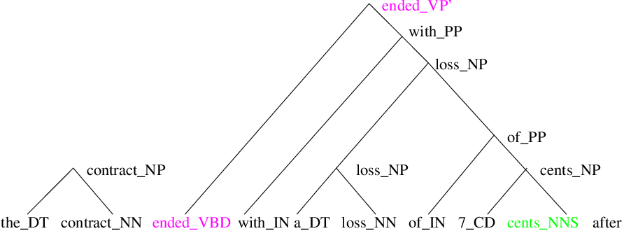
Consider predicting the word after in the sentence:
the contract ended with a loss of 7 cents
after trading as low as 89 cents.
A 3-gram approach would predict after from (7, cents)
whereas it is intuitively clear that the strongest predictor would be
contract ended which is outside the reach of even 7-grams. What
would enable us to identify the predictors in the sentence prefix?
The linguistically correct partial parse of
the sentence prefix when predicting after is shown in
Figure 4.
The word ended is called the headword of the
constituent (ended (with (...)))
and ended is an exposed headword when predicting
after — topmost headword in the largest constituent that
contains it.
Our working hypothesis is that the syntactic structure filters out irrelevant words and points to the important ones, thus enabling the use of information in the more distant past when predicting the next word. We will attempt to model this using the concept of exposed headwords introduced before.
We will give two heuristic arguments that justify the use of exposed headwords:
- •
the 3-gram context for predicting
after—(7, cents)— is intuitively less satisfying than using the two most recent exposed headwords(contract, ended)— identified by the parse tree; - •
the headword context does not change if we remove the
(of (7 cents))constituent — the resulting sentence is still a valid one — whereas the 3-gram context becomes(a, loss).
The preliminary experiments reported in [8] — although the perplexity results are conditioned on parse structure developed by human annotators by having the entire sentence at their disposal — showed the usefulness of headwords accompanied by non-terminal labels for making a better prediction of the word following a given sentence prefix.
Our model will attempt to build the syntactic structure incrementally while traversing the sentence left-to-right. The word string can be observed whereas the parse structure with headword and POS/NT label annotation — denoted by — remains hidden. The model will assign a probability to every sentence with every possible POStag assignment, binary branching parse, non-terminal label and headword annotation for every constituent of .
Let be a sentence of length words to which we have prepended
<s> and appended </s> so that <s> and
</s>.
Let be the word k-prefix of the sentence and
the word-parse k-prefix. To stress this point, a
word-parse k-prefix contains — for a given parse — those
and only those binary subtrees whose span is completely included in the word k-prefix, excluding
<s>. Single words along with their POStag can be
regarded as root-only trees. Figure 5 shows a
word-parse k-prefix; h_0 .. h_{-m} are the exposed
heads, each head being a pair(headword, non-terminal label), or
(word, POStag) in the case of a root-only tree.

A complete parse — Figure 6 — is defined as
a binary parse of the (</s>,SE)
22
2
SB is a distinguished POStag for the sentence
beginning symbol ¡s¿; SE is a distinguished POStag for the sentence
end symbol ¡/s¿;
sequence with the restriction that (</s>, TOP’) is the only
allowed head.

Note that needn’t be a constituent,
but for the parses where it is, there is no a priori restriction on which of
its words is the headword or what is the non-terminal label that
accompanies the headword. This is one other notable difference
between our model and the traditional ones developed in the
computational linguistics community imposed by the bottom-up
operation of the model. The manually annotated trees in the treebank
(see Figure 2) have all the words in a sentence
as one single constituent bearing a restricted set of non-terminal
labels: the sentence is a
constituent labeled with S.
As it can be observed the UPenn treebank -style trees are a subset of the family of trees allowed by our parameterization, making a direct comparison between our model and state of the art parsing techniques — which insist on generating UPenn treebank -style parses — less meaningful.
The model will operate by means of three modules:
- •
WORD-PREDICTOR predicts the next word given the word-parse k-prefix and then passes control to the TAGGER;
- •
TAGGER predicts the POStag of the next word given the word-parse k-prefix and the newly predicted word and then passes control to the PARSER;
- •
PARSER grows the already existing binary branching structure by repeatedly generating transitions from the following set:
(unary, NTlabel),(adjoin-left, NTlabel)or(adjoin-right, NTlabel)until it passes control to the PREDICTOR by taking anulltransition.NTlabelis the non-terminal label assigned to the newly built constituent and{left,right}specifies where the new headword is percolated from.
The operations performed by the PARSER are illustrated in Figures 9-9 and they ensure that all possible binary branching parses with all possible headword and non-terminal label assignments for the word sequence can be generated.


Algorithm 1 at the end of this chapter formalizes the above description of the sequential generation of a sentence with a complete parse.
Transition t;         // a PARSER transition
predict (<s>, SB);
do{
  //WORD-PREDICTOR and TAGGER
  predict (next_word, POStag);
  //PARSER
  do{
    if(h_{-1}.word != <s>){
      if(h_0.word == </s>)
        t = (adjoin-right, TOP’);
      else{
        if(h_0.tag == NTlabel)
          t = [(adjoin-{left,right}, NTlabel),
               null];
        else
          t = [(unary, NTlabel),
               (adjoin-{left,right}, NTlabel),
               null];
      }
    }
    else{
      if(h_0.tag == NTlabel)
        t = null;
      else
        t = [(unary, NTlabel), null];
    }
  }while(t != null) //done PARSER
}while(!(h_0.word==</s> && h_{-1}.word==<s>))
t = (adjoin-right, TOP); //adjoin <s>_SB; DONE;
The unary transition is allowed only when the most recent exposed head is a leaf of the tree — a regular word along with its POStag — hence it can be taken at most once at a given position in the input word string. The second subtree in Figure 5 provides an example of a unary transition followed by a null transition.
It is easy to see that any given word sequence with a possible parse and headword annotation is generated by a unique sequence of model actions. This will prove very useful in initializing our model parameters from a treebank.
5 Probabilistic Model
The language model operation provides an encoding of a given word sequence along with a parse tree into a sequence of elementary model actions and it can be formalized as a finite state machine (FSM) — see Figure 10. In order to obtain a correct probability assignment one has to simply assign proper conditional probabilities on each transition in the FSM that describes the model.

The probability of a word sequence and a complete parse can be broken into:
| (10) | |||||
| (11) | |||||
where:
- •
is the word-parse -prefix
- •
is the word predicted by WORD-PREDICTOR
- •
is the tag assigned to by the TAGGER
- •
is the parse structure attached to in order to generate
- •
is the number of operations the PARSER executes at position of the input string before passing control to the WORD-PREDICTOR (the -th operation at position k is the
nulltransition); is a function of - •
denotes the i-th PARSER operation carried out at position k in the word string:
(adjoin-left, NTtag),(adjoin-right, NTtag),null
Each is a valid word-parse k-prefix at position in the sentence, .
To ensure a proper probabilistic model over the set of complete parses for any sentence , certain PARSER and WORD-PREDICTOR probabilities must be given specific values33 3 Not all the paths through the FSM that describes the language model will result in a correct binary tree as defined by the complete parse, Figure 6. In order to prohibit such paths, we impose a set of constraints on the probability values of different model components, consistent with Algorithm 1:
- •
null, ifh_{-1}.word = <s>andh_{0}(</s>, TOP’)— that is, before predicting</s>— ensures that(<s>, SB)is adjoined in the last step of the parsing process; - •
- –
(adjoin-right, TOP),
ifh_0 = (</s>, TOP’)andh_{-1}.word = <s> - –
(adjoin-right, TOP’),
ifh_0 = (</s>, TOP’)andh_{-1}.word<s>
ensure that the parse generated by our model is consistent with the definition of a complete parse;
- –
- •
=
</s>ensures that the model halts with probability one.
A few comments on Eq. (10) are in order at this point. Eq. (10) assigns probability to a directed acyclic graph . Many other possible probability assignments are possible, and probably the most obvious choice would have been the factorization used in context free grammars. Our choice is dictated by its simplicity and left-to-right bottom-up operation. This also leads to a proper and very simple word level probability estimate — see Section 8 — even when pruning the set of parses .
Our factorization Eq. (10) assumes certain dependencies between the nodes in the graph . Also, in order to be able to reliably estimate the model components we need to make appropriate equivalence classifications of the conditioning part for each component, respectively. This is equivalent to making certain conditional independence assumptions which may not be — and probably are not — correct and thus have a damaging effect on the modeling power of our model.
The equivalence classification should identify the strong predictors in the context and allow reliable estimates from a treebank. Our choice is inspired by [11] and intuitively explained in Section 4:
| (12) | |||||
| (13) | |||||
| (14) |
The above equivalence classifications are limited by the severe data sparseness problem faced by the 3-gram model and by no means do we believe that they are adequate, especially that used in PARSER model (14). Richer equivalence classifications should use a probability estimation method that deals better with sparse data than the one presented in section 6. The limit in complexity on the WORD-PREDICTOR (Eq.12) also makes our model directly comparable with a 3-gram model. A few different equivalence classifications have been tried as described in section 13.1.
It is worth noting that if the binary branching structure developed by the parser were always right-branching and we mapped the POStag and non-terminal tag vocabularies to a single type, then our model would be equivalent to a trigram language model.
6 Modeling Tool
All model components — WORD-PREDICTOR, TAGGER, PARSER — are conditional probabilistic models of the type where belong to a mixed set of words, POStags, non-terminal tags and parser operations ( only). Let be the vocabulary in which the predicted random variable takes values.
For simplicity, the probability estimation method we chose was recursive linear interpolation among relative frequency estimates of different orders using a recursive mixing scheme (see Figure 11):
| (15) | |||||
| (16) | |||||
where:
- •
is the context of order when predicting ;
- •
is the order-k relative frequency estimate for the conditional probability :
- •
are the interpolation coefficients satisfying
.

The coefficients are grouped into equivalence classes — “tied” — based on the range into which the count falls; the count ranges for each equivalence class — also called “buckets” — are set such that a statistically sufficient number of events fall in that range. The approach is a standard one [18]. In order to determine the interpolation weights, we apply the deleted interpolation technique:
- •
we split the training data in two sets — “development” and
“cross-validation”, respectively; - •
we get the relative frequency — maximum likelihood — estimates
from “development” data - •
we employ the expectation-maximization (EM) algorithm [14] for determining the maximum likelihood estimate from “cross-validation” data of the “tied” interpolation weights 44 4 The “cross-validation” data cannot be the same as the development data; if this were the case, the maximum likelihood estimate for the interpolation weights would be , disallowing the mixing of different order relative frequency estimates and thus performing no smoothing at all;
We have written a general deleted interpolation tool which takes as input:
- •
joint counts gathered from the “development” and ”cross-validation data”, respectively
- •
initial interpolation values and bucket descriptors for all levels in the deleted interpolation scheme
The program runs a pre-specified number of EM iterations at each level in the deleted interpolation scheme — from bottom up, — and returns a descriptor file containing the estimated coefficients.
The descriptor file can then be used for initializing the module and thus rendering it usable for the calculation of conditional probabilities . A sample descriptor file for the deleted interpolation statistics module is shown in Table 3.
## Stats_Del_Int descriptor file
## $Id: del_int_descriptor.tex,v 1.3 1999/03/16 17:54:16 chelba Exp $
Stats_Del_Int::_main_counts_file = counts.devel.HH_w.E0.gz ;
Stats_Del_Int::_held_counts_file = counts.check.HH_w.E0.gz ;
Stats_Del_Int::_max_order = 4 ;
Stats_Del_Int::_no_iterations = 0 ;
Stats_Del_Int::_no_iterations_at_read_in = 100 ;
Stats_Del_Int::_predicted_vocabulary_chunk = 0 ;
Stats_Del_Int::_prob_Epsilon = 1e-07 ;

Stats_Del_Int::lambdas_level.0 =  2:__1__0.019 ;
Stats_Del_Int::buckets_level.0 =  2:__0__10000000 ;

Stats_Del_Int::lambdas_level.1 = 13:__1__0.5__0.5__0.5__0.5__0.5__1__1
                                    __0.449__1__0.260__0.138__0.073 ;
Stats_Del_Int::buckets_level.1 = 13:__0__1__2__4__8__16__32__64
                                    __128__256__512__1024__10000000 ;

Stats_Del_Int::lambdas_level.2 = 13:__1__0.853__0.787__0.745__0.692
                                    __0.637__0.579__0.489__0.427__0.358
                                    __0.296__0.258__0.213 ;
Stats_Del_Int::buckets_level.2 = 13:__0__1__2__4__8
                                    __16__32__64__128__256
                                    __512__1024__10000000 ;

Stats_Del_Int::lambdas_level.3 = 13:__1__0.935__0.905__0.878__0.855
                                    __0.812__0.743__0.686__0.633__0.595
                                    __0.548__0.515__0.517 ;
Stats_Del_Int::buckets_level.3 = 13:__0__1__2__4__8
                                    __16__32__64__128__256
                                    __512__1024__10000000 ;

Stats_Del_Int::lambdas_level.4 = 13:__1__0.887__0.859__0.838__0.801
                                    __0.761__0.710__0.627__0.586__0.532
                                    __0.523__0.485__0.532 ;
Stats_Del_Int::buckets_level.4 = 13:__0__1__2__4__8
                                    __16__32__64__128__256
                                    __512__1024__10000000 ;
The deleted interpolation method is not optimal for our problem. Our models would require a method able to optimally combine the predictors of different nature in the conditioning part of the model and this is far from being met by the fixed hierarchical scheme used for context mixing in deleted interpolation estimation. The best method would be maximum entropy [5] but due to its computational burden we have not used it.
7 Pruning Strategy
Since the number of parses for a given word prefix grows faster than exponential55 5 Thanks to Bob Carpenter, Lucent Technologies Bell Labs, for pointing out this inaccuracy in our [9] paper with , , the state space of our model is huge even for relatively short sentences. We thus have to prune most parses without discarding the most likely ones for a given prefix . Our pruning strategy is a synchronous multi-stack search algorithm.
Each stack contains hypotheses — partial parses — that have been constructed by the same number of predictor and the same number of parser operations. The hypotheses in each stack are ranked according to the score, highest on top. The amount of search is controlled by two parameters:
- •
the maximum stack depth — the maximum number of hypotheses the stack can contain at any given time;
- •
log-probability threshold — the difference between the log-probability score of the top-most hypothesis and the bottom-most hypothesis at any given state of the stack cannot be larger than a given threshold.
Figure 12 shows schematically the operations associated with the scanning of a new word 66 6 is the maximum number of adjoin operations for a k-length word prefix; since the tree is binary we have .

First, all hypotheses in a given stack-vector are expanded with the following word. Then, for each possible POS tag the following word can take, we expand the hypotheses further. Due to the finite stack size, some are discarded. We then proceed with the PARSER expansion cycle, which takes place in two steps:
- 1.
first all hypotheses in a given stack are expanded with all possible PARSER actions excepting the
nulltransition. The resulting hypotheses are sent to the immediately lower stack of the same stack-vector — same number of WORD-PREDICTOR operations and exactly one more PARSER move. Some are discarded due to finite stack size. - 2.
after completing the previous step, all resulting hypotheses are expanded with the
nulltransition and sent into the next stack-vector. Pruning can still occur due to the log-probability threshold on each stack.
current_stack_vector // set of stacks at current input position
future_stack_vector  // set of stacks at future  input position
hypothesis           // initial hypothesis
stack                // initial empty stack

// initialize algorithm
insert hypothesis in stack;
push stack at end of current_stack_vector;

// traverse input sentence
for each position in input sentence{
  PREDICTOR and TAGGER extension cycle;
  current_stack_vector = future_stack_vector;
  erase future_stack_vector;

  PARSER extension cycle;
  current_stack_vector = future_stack_vector;
  erase future_stack_vector;
}
// output the hypothesis with the highest score;
output max scoring hypothesis in current_stack_vector;
current_stack_vector // set of stacks at current input position
future_stack_vector  // set of stacks at future  input position
word                 // word at current input position
for each stack in current_stack_vector{
  // based on number of predictor and parser operations
  identify corresponding future_stack in future_stack_vector;

  for each hypothesis in stack{
    for all possible POStag assignments for word{ //CACHE-ING
      expand hypothesis with word, POStag;
      insert hypothesis in future_stack;
    }
  }
}
current_stack_vector // set of stacks at current input position
future_stack_vector  // set of stacks at future  input position

// all possible parser transitions but the null-transition
for each stack in current_stack_vector, from bottom up{
  // based on number of parser operations
  identify corresponding future_stack in current_stack_vector;
  for each hypothesis in current_stack{         // HARD PRUNING
    for each parser_transition except the null-transition{//CACHE-ING
      expand hypothesis with parser_transition;
      insert hypothesis in future_stack;
    }
  }
}
// null-transition moves us to the next position in the input
for each stack in current_stack_vector{
  // based on number of predictor and parser operations
  identify corresponding future_stack in future_stack_vector;
  for each hypothesis in current_stack{
    expand hypothesis with null-transition;
    insert hypothesis in future_stack;
  }
}
prune future_stack_vector                 //SECOND PRUNING STEP
7.0.1 Second Pruning Step
The pruning strategy described so far proved to be
insufficient77
7
Assuming that all stacks contain the maximum
number of entries — equal to the stack-depth — the search effort
grows squared with the sentence length so in order to approximately
linearize the search effort with respect to sentence length, we chose
to discard also the hypotheses whose score is more than a fixed
log-probability relative threshold below the score of the topmost
hypothesis in the current stack vector. This additional pruning step
is performed after all hypotheses in stage have been extended
with the null parser transition.
7.0.2 Cashed TAGGER and PARSER Lists
Another opportunity for speeding up the search is to have a cached list of possible POStags/parser-operations in a given TAGGER/PARSER context. A good cache-ing scheme should use an equivalence classification of the context that is specific enough to actually reduce the list of possible options and general enough to apply in almost all the situations. For the TAGGER model we cache the list of POStags for a given word seen in the training data and scan only those in the TAGGER extension cycle — see Algorithm 3. For the PARSER model we cache the list of parser operations seen in a given context in the training data; parses that expose heads whose pair of NTtags has not been seen in the training data are discarded— see Algorithm 4.
8 Word Level Perplexity
Attempting to calculate the conditional perplexity by assigning to a whole sentence the probability:
| (17) |
where — the search for being carried out according to our pruning strategy — is not valid because it is not causal: when predicting we would be using which was determined by looking at the entire sentence. To be able to compare the perplexity of our model with that resulting from the standard trigram approach, we would need to factor in the entropy of guessing the prefix of the final best parse before predicting , based solely on the word prefix .
To maintain a left-to-right operation of the language model, the probability assignment for the word at position in the input sentence was made using:
| (18) | |||||
where is the set of all parses present in our stacks at the current stage . This leads to the following formula for evaluating the perplexity:
| (19) |
Note that if we set — 0-entropy guess for the prefix of the parse to equal that of the final best parse — the two probability assignments (17) and (18) would be the same, yielding a lower bound on the perplexity achievable by our model when using a given pruning strategy.
Another possibility for evaluating the word level perplexity of our model is to approximate the probability of a whole sentence:
| (20) |
where is one of the “N-best” — in the sense defined by our search — parses for . This is a deficient probability assignment, however useful for justifying the model parameter re-estimation to be presented in Chapter 3.
The two estimates (18) and (20) are both consistent in the sense that if the sums are carried over all possible parses we get the correct value for the word level perplexity of our model.
Another important observation is that the next-word predictor
probability
in (18)
need not be the same as the WORD-PREDICTOR
probability (12) used to extract the structure
, thus leaving open the possibility of estimating it
separately. To be more specific, we can in principle have a
WORD-PREDICTOR model component that operates within the parser model
whose role strictly to extract syntactic structure and a second model
that is used only for the left to right probability assignment:
| (21) | |||||
| (22) |
In this case the interpolation coefficient given by 22 uses the regular WORD-PREDICTOR model whereas the prediction of the next word for the purpose of word level probability assignment is made using a separate model .
Chapter 3 Structured Language Model Parameter Estimation
As outlined in section 8, the word level probability assigned to a training/test set by our model is calculated using the proper word-level probability assignment in equation (18). An alternative which leads to a deficient probability model is to sum over all the complete parses that survived the pruning strategy, formalized in equation (20). Let the likelihood assigned to a corpus by our model be denoted by:
- •
, where is calculated using (18), repeated here for clarity:
Note that this is a proper probability model.
- •
, where is calculated using (20):
This is a deficient probability model: due to the fact that we are not summing over all possible parses for a given word sequence — we discard most of them through our pruning strategy — we underestimate the probability and thus .
One seeks to devise an algorithm that finds the model parameter values which maximize the likelihood of a test corpus. This is an unsolved problem; the standard approach is to resort to maximum likelihood estimation techniques on a training corpus and make provisions that will ensure that the increase in likelihood on training data carries over to unseen test data.
In our case we would like to estimate the model component probabilities (12 – 14). The smoothing scheme outlined in Section 6 is intended to prevent overtraining and tries to ensure that maximum likelihood estimates on the training corpus will carry over to test data. Since our problem is one of maximum likelihood estimation from incomplete data — the parse structure along with POS/NT tags and headword annotation for a given observed sentence is hidden — our approach will make heavy use of the EM algorithm variant presented in chapter 9.
The estimation procedure proceeds in two stages: first the “N-best training” algorithm (see Section 10) is employed to increase the training data “likelihood” ; we rely on the consistency property outlined at the end of Section 8 to correlate the increase in with the desired increase of . The initial parameters for this first estimation stage are gathered from a treebank as described in Section 10.1.
The second stage estimates the model parameters such that is increased. The basic idea is to realize that the WORD-PREDICTOR in the structured language model (as described in chapter 2) and that used for word prediction in the calculation can be estimated as two separate components: one that is used for structure generation and a second one which is used strictly for predicting the next word as described in equation (18). The initial parameters for the second component are obtained by copying the WORD-PREDICTOR estimated at stage one.
As a final step in refining the model we have linearly interpolated the structured language model (18) with a trigram model. Results and comments on them are presented in the last section of the chapter.
9 Maximum Likelihood Estimation from Incomplete Data
In many practical situations we are confronted with the following situation: we are given a collection of data points — training data — which we model as independent samples drawn from the marginal of the parametric distribution:
where is referred to as the hidden variable and as the hidden event space, respectively. The set
is referred to as the model set. Let be the relative frequency probability distribution induced on by the collection .
We wish to find the maximum-likelihood estimate of :
| (23) | |||||
| (24) |
Starting with an initial parameter value , it is shown that a sufficient condition for increasing the likelihood of the training data (see Eq. 23) is to find a new parameter value that maximizes the so called EM auxiliary function defined as:
| (25) |
The EM theorem proves that choosing:
| (26) |
ensures that the likelihood of the training data under the new parameter value is not lower than that under the old one, formally:
| (27) |
Under more restrictive conditions on the model family it can be shown that the fixed points of the EM procedure — — are in fact local maxima of the likelihood function . The study of convergence properties under different assumptions on the model class as well as different flavors of the EM algorithm is an open area of research.
The fact that the algorithm is naturally formulated to operate with probability distributions — although this constraint can be relaxed — makes it attractive from a computational point of view: an alternative to maximizing the training data likelihood would be to apply gradient maximization techniques; this may be particularly difficult if not impossible when the analytic description of the likelihood as a function of the parameter is complicated.
To further the understanding of the computational aspects of using the EM algorithm we notice that the EM update (26) involves two steps:
- •
E-step: for each sample in the training data , accumulate the expectation of under the distribution ; no matter what the actual analytic form of is, this requires to traverse all possible derivations of the seen event that have non-zero conditional probability ;
- •
M-step: find maximizer of the auxiliary function (25).
Typically the M-step is simple and the computational bottleneck is the E-step. The latter becomes intractable with large training data set size and rich hidden event space, as usually required by practical problems.
In order to overcome this limitation, the model space is usually structured such that dynamic programming techniques can be used for carrying out the E-step — see for example the hidden Markov model(HMM) parameter reestimation procedure [3]. However this advantage does not come for free: in order to be able to structure the model space we need to make independence assumptions that weaken the modeling power of our parameterization. Fortunately we are not in a hopeless situation: a simple modification of the EM algorithm allows the traversal of only a subset of all possible for each training sample — the procedure is dubbed “N-best training“ — thus rendering it applicable to a much broader and more powerful class of models.
9.1 N-best Training Procedure
Before proceeding with the presentation of the N-best training procedure, we would like to introduce a view of the EM algorithm based on information geometry. Having gained this insight we can then easily justify the N-best training procedure. This is an interesting area of research to which we were introduced by the presentation in [6].
9.1.1 Information Geometry and EM
The problem of maximum likelihood estimation from incomplete data can be viewed in an interesting geometric framework. Before proceeding, let us introduce some concepts and the associated notation.
Alternating Minimization
Consider the problem of finding the minimum Euclidean distance between two convex sets A and B:
| (28) |

The following iterative procedure(see figure 13) should lead to the solution: start with a random point ; find the point closest to ; then fix and find the point closest to and so on. It is intuitively clear that the distance between the two points considered at each iteration cannot increase and that the fixed point of the above procedure — the choice for the points does not change from one iteration to the next — is the minimum distance between the sets and .
Formalizing this intuition proves to be less simple for a more general setup — the specification of sets and and the distance used. Csiszar and Tusnady have derived sufficient conditions under which the above alternating minimization procedure converges to the minimum distance between the two sets [13]. As outlined in [12], this algorithm is applicable to problems in information theory — channel capacity and rate distortion calculation — as well as in statistics — the EM algorithm.
EM as alternating minimization
Let be the family of probability distributions from which we want to choose the one maximizing the likelihood of the training data (23). Let us also define a family of desired distributions on whose marginal induced by the training data is the same as the relative frequency estimate :
For any pair , the Kullback-Leibler distance (KL-distance) between and is defined as:
| (29) |
As shown in [13], under certain conditions on the families and and using the KL-distance, the alternating minimization procedure described in the previous section converges to the minimum distance between the two sets:
| (30) |
It can be easily shown (see appendix 8) that the model distribution that satisfies (30) is also the one maximizing the likelihood of the training data,
Moreover, the alternating minimization procedure leads exactly to the EM update equation(25, 26), as shown in [13] and sketched in appendix 9.
The and families one encounters in practical situations may not satisfy the conditions specified in [13]. However, one can easily note that decrease in at each step and correct I-projection from to — finding such that we minimize — are sufficient conditions for ensuring that the likelihood of the training data does not decrease with each iteration. Since in practice we are bound by computational limitations and we typically run just a few iterations, the guaranteed non-decrease in training data likelihood is sufficient.
9.2 N-best Training
In the “N-best” training paradigm we use only a subset of the conditional hidden event space , for any given seen . Associated with the model space we now have a family of strategies to sample from a set of “N-best” hidden events , for any . The family is parameterized by :
| (31) |
With the following definitions:
| (32) | |||||
| (33) | |||||
| (34) |
the alternating minimization procedure between and using the KL-distance will find a sequence of parameter values for which the “likelihood”:
| (35) |
is monotonically increasing: . Note that due to the truncation of we are dealing with a deficient probability model.
The parameter update at each iteration is very similar to that specified by the EM algorithm under some sufficient conditions, as specified in Proposition 1 and proved in Appendix 10:
Proposition 1
Assuming that (“smooth” ) holds, one alternating minimization step between and — — is equivalent to:
| (36) |
if satisfies:
| (37) |
Only are candidates in the M-step.
The fact that we are working with a deficient probability model for which the support of the distributions cannot decrease from one iteration to the next makes the above statement less interesting: even if we didn’t substantially change the model parameters from one iteration to the next— — but we chose the sampling function such that the “likelihood” would still be increasing due to the support expansion, although the quality of the model has not actually increased.
In practice the family of sampling functions (31) is chosen such that support of has constant size — cardinality, for discrete hidden spaces. Typically one retains the “N-best” after ranking the hidden sequences in decreasing order according to . Proposition 1 implies that the set of “N-best” should not change from one iteration to the next, being an invariant during model parameter reestimation. In practice however we recalculate the “N-best” after each iteration, allowing the possibility that new hidden sequences are being included in the “N-best” list at each iteration and others discarded. We do not have a formal proof that this procedure will ensure monotonic increase of the “likelihood” .
10 First Stage of Model Estimation
Let denote the joint sequence of with parse structure — headword and POS/NT tag annotation included. As described in section 4, was produced by a unique sequence of model actions: word-predictor, tagger, and parser moves. The ordered collection of these moves will be called a derivation:
where each elementary event
identifies a model component action:
- •
denotes the model component that took the action,
WORD-PREDICTOR, TAGGER, PARSER ; - •
is the action taken:
- –
is a word for WORD-PREDICTOR;
- –
is a POS tag for TAGGER;
- –
(adjoin-left, NTtag),(adjoin-right, NTtag),null
for PARSER;
- –
- •
For each given which satisfies the requirements in section 4 there is a unique derivation . The converse is not true, namely not every derivation corresponds to a correct ; however, the constraints in section 5 ensure that these derivations receive 0 probability.
The probability of a sequence is obtained by chaining the probabilities of the elementary events in its derivation, as described in section 5:
| (38) |
The probability of an elementary event is calculated using the smoothing technique presented in section 6 and repeated here for clarity of explanation:
| (39) | |||||
| (40) | |||||
- •
is the context of order when predicting ; is the vocabulary in which takes values;
- •
is the order-k relative frequency estimate for the conditional probability :
- •
are the interpolation coefficients satisfying .
The coefficients are grouped into equivalence classes — “tied” — based on the range into which the count falls; the count ranges for each equivalence class are set such that a statistically sufficient number of events fall in that range.
The parameters of a given model component are:
- •
the maximal order counts ;
- •
the count ranges for grouping the interpolation values into equivalence classes — “tying”;
- •
the interpolation value for each equivalence class;
Assuming that the count ranges and the corresponding interpolation values for each order are kept fixed to their initial values — see section 10.1 — the only parameters to be reestimated using the EM algorithm are the maximal order counts for each model component.
In order to avoid traversing the entire hidden space for a given observed word sequence88 8 normally required in the E-step we use the “N-best” training approach presented in section 9.1 for which the sampling strategy is the same as the pruning strategy presented in section 7.
The derivation of the reestimation formulas is presented in appendix 11. The E-step is the one presented in section 9.2; the M-step takes into account the smoothing technique presented above (equation (39)).
Note that due to both the smoothing involved in the M-step and the fact that the set of sampled “N-best” hidden events — parses — are reevaluated at each iteration we allow new maximal order events to appear in each model component while discarding others. Not only are we estimating the counts of maximal order n-gram events in each model component — WORD-PREDICTOR, TAGGER, PARSER — but we also allow the distribution on types to change from one iteration to the other. This is because the set of hidden events allowed for a given observed word sequence is not invariant — as it is the case in regular EM. For example, the count set that describes the WORD-PREDICTOR component of the model to be used at the next iteration is going to have a different n-gram composition than that used at the current iteration. This change is presented in the experiments section, see Table 7.
10.1 First Stage Initial Parameters
Each model component — WORD-PREDICTOR, TAGGER, PARSER — is initialized from a set of hand-parsed sentences — in this case are going to use the UPenn Treebank manually annotated sentences — after undergoing headword percolation and binarization, as explained in section 3.1. This is a subset — approx. 90% — of the training data. Each parse tree is then decomposed into its derivation . Separately for each model component, we:
- •
gather joint counts from the derivations that make up the “development data” using (see appendix 11);
- •
estimate the interpolation coefficients on joint counts gathered from “check data” — the remaining 10% of the training data — using the EM algorithm [14].
These are the initial parameters used with the reestimation procedure described in the previous section.
11 Second Stage Parameter Reestimation
In order to improve performance, we develop a model to be used strictly for word prediction in (18), different from the WORD-PREDICTOR model (12). We will call this new component the L2R-WORD-PREDICTOR.
The key step is to recognize in (18) a hidden Markov model (HMM) with fixed transition probabilities — although dependent on the position in the input sentence — specified by the values.
The E-step of the EM algorithm [14] for gathering joint counts , L2R-WORD-PREDICTOR-MODEL, is the standard one whereas the M-step uses the same count smoothing technique as that described in section 10.
The second reestimation pass is seeded with the WORD-PREDICTOR model joint counts resulting from the first parameter reestimation pass (see section 10).
Chapter 4 Experiments using the Structured Language Model
For convenience, we chose to work on the UPenn
Treebank corpus [21] — a subset of the WSJ (Wall Street
Journal) corpus.
The vocabulary sizes were:
word vocabulary: 10k, open — all words outside the vocabulary are
mapped to the <unk> token; POS tag vocabulary: 40, closed;
non-terminal tag vocabulary: 52, closed; parser operation vocabulary:
107, closed. The training data was split into development set
(929,564wds (sections 00-20)), check set (73,760wds (sections 21-22))
and the test data consisted of 82,430wds (sections 23-24). The “check”
set was used strictly for initializing the model parameters as
described in section 10.1; the
“development” set was used with the reestimation techniques described in
chapter 3.
12 Perplexity Results
Table 4 shows the results of the reestimation techniques; E0-3 and
L2R0-5 denote iterations of the reestimation procedure
described in sections 10 and
11, respectively. A deleted
interpolation trigram model derived from the same training data had
perplexity 167.14 on the same test data.
| iteration | DEV set | TEST set |
|---|---|---|
| number | L2R-PPL | L2R-PPL |
| E0 | 24.70 | 167.47 |
| E1 | 22.34 | 160.76 |
| E2 | 21.69 | 158.97 |
| E3 = L2R0 | 21.26 | 158.28 |
| L2R5 | 17.44 | 153.76 |
Simple linear interpolation between our model and the trigram model:
yielded a further improvement in PPL, as shown in Table 5. The interpolation weight was estimated on check data to be . An overall relative reduction of 11% over the trigram model has been achieved.
| iteration | TEST set | TEST set |
|---|---|---|
| number | L2R-PPL | 3-gram interpolated PPL |
| E0 | 167.47 | 152.25 |
| E3 | 158.28 | 148.90 |
| L2R5 | 153.76 | 147.70 |
As outlined in section 8, the perplexity value calculated using (17):
is a lower bound for the achievable perplexity of our model; for the above search parameters and E3 model statistics this bound was 99.60, corresponding to a relative reduction of 41% over the trigram model. This suggests that a better parameterization in the PARSER model — one that reduces the entropy of guessing the “good” parse given the word prefix — can lead to a better model. Indeed, as we already pointed out, the trigram model is a particular case of our model for which the parse is always right branching and we have no POS/NT tag information, leading to and a standard 3-gram WORD-PREDICTOR. The 3-gram model is thus an extreme case of the structured language model: one for which the “hidden” structure is a function of the word prefix. Our result shows that better models can be obtained by allowing richer “hidden” structure — parses — and that a promising direction of research may be to find the best compromise between the predictive power of the WORD-PREDICTOR — measured by — and the ease of guessing the hidden structure — measured by — on which the WORD-PREDICTOR operation is based. A better solution would be a maximum entropy PARSER model which incorporates a richer set of predictors in a better way than the deleted interpolation scheme we are using. Due to the computational problems faced by such a model we have not pursued this path although we consider it a very promising one.
12.1 Comments and Experiments on Model Parameters Reestimation
The word level probability assigned to a training/test set by our model is calculated using the proper word-level probability assignment in equation (18). An alternative which leads to a deficient probability model is to sum over all the complete parses that survived the pruning strategy, formalized in equation (20). Let the likelihood assigned to a corpus by our model be denoted by:
- •
, where is calculated using (18), repeated here for clarity:
Note that this is a proper probability model.
- •
One seeks to devise an algorithm that finds the model parameter values which maximize the likelihood of a test corpus. This is an unsolved problem; the standard approach is to resort to maximum likelihood estimation techniques on the training corpus and make provisions that will ensure that the increase in likelihood on training data carries over to unseen test data.
As outlined previously, the estimation procedure of the SLM parameters takes place in two stages:
- 1.
- 2.
estimate a separate L2R-WORD-PREDICTOR model such that is increased — see Eq. (21). The initial parameters for the L2R-WORD-PREDICTOR component are obtained by copying the WORD-PREDICTOR estimated at stage one.
As explained in Section 12.1, the “N-best training” algorithm is employed to increase the training data “likelihood” ; we rely on the consistency of the probability estimates underlying the calculation of the two different likelihoods to correlate the increase in with the desired increase of .
To be more specific, and are calculated using the probability assignments in Eq. (20) — deficient — and Eq. (18), respectively. Both probability estimates are consistent in the sense that if we summed over all the parses for a given word sequence they would yield the correct probability according to our model. Although there is no formal proof, there are reasons to believe that the N-best reestimation procedure should not decrease the likelihood 99 9 It is very similar to a rigorous EM approach but no claim can be made about the increase in the likelihood — which is the one we are interested in. Our experiments show that the increase in is correlated with an increase in , a key factor in this being a good heuristic search strategy — see Section 7. Table 6 shows the evolution of different “perplexity” values during N-best reestimation. L2R-PPL is calculated using the proper probability assignment in Eq.(18). TOP-PPL and BOT-PPL are calculated using the probability assignment in Eq.(17), where and , respectively — the search for being carried out according to our pruning strategy; we condition the word predictions on the topmost and bottom-most parses present in the stacks after parsing the entire sentence. SUM-PPL is calculated using the deficient probability assignment in Eq.(20). It can be noticed that TOP-PPL and BOT-PPL stay almost constant during the reestimation process; The value of TOP-PPL is slightly increasing and that of BOT-PPL is slightly decreasing. As expected, the value of the SUM-PPL decreases and its decrease is correlated with that of the L2R-PPL.
| “Perplexity” | Iteration | Relative Change | |
| E0 | E3 | ||
| TOP-PPL | 97.5 | 99.3 | +1.85% |
| BOT-PPL | 107.9 | 106.2 | -1.58% |
| SUM-PPL | 195.1 | 175.5 | -10.05% |
| L2R-PPL | 167.5 | 158.3 | -5.49% |
It is very important to note that due to both the smoothing involved in the M-step --- imposed by the smooth parameterization of the model1010 10 Unlike standard parameterizations, we do not reestimate the relative frequencies from which each component probabilistic model is derived; that would lead to a shrinking or, at best, fixed set of events — and the fact that the set of sampled “N-best” hidden events — parses — are reevaluated at each iteration, we allow new maximal order events to appear in each model component while discarding others. Not only are we estimating the counts of maximal order n-gram events in each model component — WORD-PREDICTOR, TAGGER, PARSER — but we also allow the distribution on types to change from one iteration to the other. This is because the set of hidden events allowed for a given observed word sequence is not invariant. For example, the count set that describes the WORD-PREDICTOR component of the model to be used at the next iteration may have a different n-gram composition than that used at the current iteration.
We evaluated the change in the distribution on types1111 11 A type is a particular value, regarded as one entry in the alphabet spanned by a given random variable of the maximal order events from one iteration to the next. Table 7 shows the dynamics of the set of types of the different order events during the reestimation process for the WORD-PREDICTOR model component. Similar dynamics were observed for the other two components of the model. The equivalence classifications corresponding to each order is:
- •
for order 4;
- •
for order 3;
- •
for order 2;
- •
for order 1;
An event of order 0 consists of the predicted word only.
| iteration | no. tokens | no. types for order | ||||
|---|---|---|---|---|---|---|
| 0 | 1 | 2 | 3 | 4 | ||
| E0 | 929,564 | 9,976 | 77,225 | 286,329 | 418,843 | 591,505 |
| E1 | 929,564 | 9,976 | 77,115 | 305,266 | 479,107 | 708,135 |
| E2 | 929,564 | 9,976 | 76,911 | 305,305 | 482,503 | 717,033 |
| E3 | 929,564 | 9,976 | 76,797 | 307,100 | 490,687 | 731,527 |
| L2R0 (=E3) | 929,564 | 9,976 | 76,797 | 307,100 | 490,687 | 731,527 |
| L2R1-5 | 929,564 | 9,976 | 257,137 | 2,075,103 | 3,772,058 | 5,577,709 |
The higher order events — closer to the root of the linear interpolation scheme in Figure 11 — become more and more diverse during the first estimation stage, as opposed to the lower order events. This shows that the “N-best” parses for a given sentence change from one iteration to the next. Although the E0 counts were collected from “1-best” parses — binarized treebank parses — the increase in number of maximal order types from E0 to E1 — collected from “N-best”, N = 10 — is far from dramatic, yet higher than that from E1 to E2 — both collected from “N-best” parses.
The big increase in number of types from E3 (=L2R0) to L2R1 is due to the fact that at each position in the input sentence, WORD-PREDICTOR counts are now collected for all the parses in the stacks, many of which do not belong to the set of N-best parses for the complete sentence used for gathering counts during E0-3.
Although the perplexity on test data still decreases during the second reestimation stage — we are not over-training — this decrease is very small and not worth the computational effort if the model is linearly interpolated with a 3-gram model, as shown in Table 5. Better integration of the 3-gram and the head predictors is desirable.
13 Miscellaneous Other Experiments
13.1 Choosing the Model Components Parameterization
The experiments presented in [8] show the usefulness of the two most recent exposed heads for word prediction. The same criterion — conditional perplexity — can be used as a guide in selecting the parameterization of each model component: WORD-PREDICTOR, TAGGER, PARSER. For each model component we gather the counts from the UPenn Treebank as explained in Section 10.1. The relative frequencies are determined from the “development” data, the interpolation weights estimated on “check” data — as described in Section 10.1. We then test each model component on counts gathered from the “test” data. Note that the smoothing scheme described in Section 6 discards elements of the context from right to left.
13.1.1 Selecting the WORD-PREDICTOR Equivalence Classification
The experiments in [8] were repeated using deleted interpolation as a modeling tool and the training/testing setup described above. The results for different equivalence classifications of the word-parse k-prefix are presented in Table 8.
| Equivalence Classification | Cond. PPL | Voc. Size | |
|---|---|---|---|
| HH | 115 | 10,000 | |
| WW | 156 | 10,000 | |
| hh | 154 | 10,000 | |
| ww | 167 | 10,000 | |
The different equivalence classifications of the word-parse k-prefix retain the following predictors:
- 1.
ww: the two previous words — regular 3-gram model;
- 2.
hh: the two most recent exposed headwords — no POS/NT label information;
- 3.
WW: the two previous exposed words along with their POS tags;
- 4.
HH: the two most recent exposed heads — headwords along with their NT/POS labels;
It can be seen that the most informative predictors for the next word are the exposed heads --- HH model. Except for the ww model1212 12 regular 3-gram model, none of the others is a valid word-level perplexity since it conditions the prediction on hidden information (namely the tags present in the treebank parses); the entropy of guessing the hidden information would need to be factored in.
13.1.2 Selecting the TAGGER Equivalence Classification
The results for different equivalence classifications of the word-parse k-prefix for the TAGGER model are presented in Table 9.
| Equivalence Classification | Cond. PPL | Voc. Size | |
|---|---|---|---|
| HHw | 1.23 | 40 | |
| WWw | 1.24 | 40 | |
| ttw | 1.24 | 40 | |
The different equivalence classifications of the word-parse k-prefix retain the following predictors:
- 1.
WWw: the two previous exposed words along with their POS tags and the word to be tagged;
- 2.
HHw: the two most recent exposed heads — headwords along with their NT/POS labels and the word to be tagged;
- 3.
ttw: the NT/POS labels of the two most recent exposed heads and the word to be tagged;
It can be seen that among the equivalence classifications considered, none performs significantly better than the others, and the prediction of the POS tag for a given word is a relatively easy task — the conditional perplexities are very close to one. Because of its simplicity, we chose to work with the ttw equivalence classification.
13.1.3 Selecting the PARSER Equivalence Classification
The results for different equivalence classifications of the word-parse k-prefix for the PARSER model are presented in Table 10.
| Equivalence Classification | Cond. PPL | Voc. Size | |
|---|---|---|---|
| HH | 1.68 | 107 | |
| hhtt | 1.54 | 107 | |
| tt | 1.71 | 107 | |
The different equivalence classifications of the word-parse k-prefix retain the following predictors:
- 1.
HH: the two most recent exposed heads — headwords along with their NT/POS labels and the word to be tagged;
- 2.
hhtt: same as HH just that the backing-off order is changed;
- 3.
ttw: the NT/POS labels of the two most recent exposed heads;
It can be seen that the presence of headwords improves the accuracy of the PARSER component; also, the backing-off order of the predictors is important — hhtt vs. HH. We chose to work with the hhtt equivalence classification.
13.2 Fudged TAGGER and PARSER Scores
The probability values for the three model components fall into different ranges. As pointed out at the beginning of this chapter, the WORD-PREDICTOR vocabulary is of the order of thousands whereas the TAGGER and PARSER have vocabulary sizes of the order of tens. This leads to the undesirable effect that the contribution of the TAGGER and PARSER to the overall probability of a given partial parse is very small compared to that of the WORD-PREDICTOR. We explored the idea of bringing the probability values into the same range by fudging the TAGGER and PARSER probability values, namely:
| (41) | |||||
| (42) | |||||
where is the fudge factor. For we do not have a valid probability assignment anymore, however the L2R-PPL calculated using Eq. (18) is still a valid word-level probability assignment due to the re-normalization of the interpolation coefficients. Table 11 shows the PPL values calculated using Eq. (18) where is calculated using Eq. (41). As it can be seen the optimal fudge factor turns out to be 1.0, corresponding to the correct calculation of the probability .
| fudge | 0.01 | 0.02 | 0.05 | 0.1 | 0.2 | 0.5 | 1.0 | 2.0 | 5.0 | 10.0 | 20.0 | 50.0 | 100.0 |
|---|---|---|---|---|---|---|---|---|---|---|---|---|---|
| PPL | 341 | 328 | 296 | 257 | 210 | 168 | 167 | 189 | 241 | 284 | 337 | 384 | 408 |
13.3 Maximum Depth Factorization of the Model
The word level probability assignment used by the SLM — Eq. (18) — can be thought of as a model factored over different maximum reach depths. Let be the “depth” in the word-prefix at which the headword can be found.
Eq. (18) can be rewritten as:
| (43) | |||||
| where: | |||||
We can interpret Eq. (43) as a linear interpolation of models that reach back to different depths in the word prefix . The expected value of shows how far does the SLM reach in the word prefix:
| (44) |
For the 3-gram model we have . We evaluated the expected depth of the SLM using the formula in Eq. (44). The results are presented in Table 12.
| iteration | expected depth |
|---|---|
| number | E[D] |
| E0 | 3.35 |
| E1 | 3.46 |
| E2 | 3.45 |
It can be seen that the memory of the SLM is considerably higher than that of the 3-gram model — whose depth is 2.
Figure 14 shows 1313 13 The nonzero value of is due to the fact that the prediction of the first word in a sentence is based on context of length 1 in both SLM and 3-gram models the distribution , averaged over all positions in the test string:
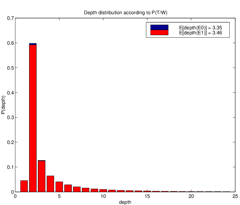
It can be seen that the SLM makes a prediction which reaches farther than the 3-gram model in about 40% of cases, on the average.
Chapter 5 Decoder for Lattices
14 Two Pass Decoding Techniques
In a two-pass recognizer, a computationally cheap decoding step is run in the first pass, a set of hypotheses is retained as an intermediate result and then a more sophisticated recognizer is run over these in a second pass — usually referred to as the rescoring pass. The search space in the second pass is much more restricted compared to the first pass so we can afford using better — usually also computationally more intensive — acoustic and/or language models.
The two most popular two-pass strategies differ mainly in the number of intermediate hypotheses saved after the first pass and the form in which they are stored.
In the so-called ‘‘N-best1414 14 The value of N is typically 100–1000 rescoring” method, a list of complete hypotheses along with acoustic/language model scores are retained and then rescored using more complex acoustic/language models.
Due to the limited number of hypotheses in the N-best list, the second pass recognizer might be too constrained by the first pass so a more comprehensive list of hypotheses is often needed. The alternative preferred to N-best list rescoring is “lattice rescoring”. The intermediate format in which the hypotheses are stored is now a directed acyclic graph in which the nodes are a subset of the language model states in the composite hidden Markov model and the arcs are labeled with words. Typically, the first pass acoustic/language model scores associated with each arc — or link — in the lattice are saved and the nodes contain time alignment information.
For both cases one can calculate the “oracle” word error rate: the word error rate along the hypothesis with the minimum number of errors. The oracle-WER decreases with the number of hypotheses saved.
Of course, a set of N-best hypotheses can be assembled as a lattice, the difference between the two being just in the number of different hypotheses — with different time-alignments — stored in the lattice. One reason which makes the N-best rescoring framework attractive is the possibility to use “whole sentence” language models: models that are able to assign a score only to complete sentences due to the fact that they do not operate in a left-to-right fashion. The drawbacks are that the number of hypotheses explored is too small and their quality reminiscent of the models used in the first pass. To clarify the latter assertion, assume that the second pass language model to be applied is dramatically different from the one used in the first pass and that if we afforded to extract the N-best using the better language model they would have a different kind of errors, specific to this language model. In that case simple rescoring of the N-best list generated using the weaker language model may constrain too much the stronger language model used in the second pass, not allowing it to show its merits.
It is thus desirable to have a sample of the possible word hypotheses which is as complete as possible — not biased towards a given model — and at the same time of manageable size. This is what makes lattice rescoring the chosen method in our case, hoping that simply by increasing the number of hypotheses retained one reduces the bias towards the first pass language model.
15 Algorithm
The algorithm [22] is a tree search strategy that could be compared to depth-first tree-traversal: pursue the most promising path as deeply as possible.
Let a set of hypotheses
be organized as a prefix tree. We wish to obtain the maximum scoring hypothesis under the scoring function :
without scoring all the hypotheses in , if possible with a minimal computational effort.
The algorithm operates with prefixes and suffixes of hypotheses in the set ; we will denote prefixes — anchored at the root of the tree — with and suffixes — anchored at a leaf — with . A complete hypothesis can be regarded as the concatenation of a prefix and a suffix: . We assume that the function can be evaluated at any prefix , i.e. is a meaningful quantity.
To be able to pursue the most promising path, the algorithm needs to evaluate all the possible suffixes for a given prefix that are allowed in — see figure 15. Let be the set of suffixes allowed by the tree for a prefix and assume we have an overestimate for the score of any complete hypothesis , :
Imposing the condition that for empty , we have
that is, the overestimate becomes exact for complete hypotheses .

Let the ranking function be defined as:
| (45) | |||||
| (46) |
is an overestimate for the score of any complete hypothesis that has the prefix ; the overestimate becomes exact for complete hypotheses:
| (47) | |||||
| (48) |
The algorithm uses a potentially infinite stack1515 15 The stack need not be larger than in which prefixes are ordered in decreasing order of the ranking function 1616 16 In fact any overestimate satisfying both Eq. (47) and (48) will ensure correctness of the algorithm; at each extension step the top-most prefix is popped form the stack, expanded with all possible one-symbol continuations of in and then all the resulting expanded prefixes — among which there may be complete hypotheses as well — are inserted back into the stack. The stopping condition is: whenever the popped hypothesis is a complete one, retain it as the overall best hypothesis — see Algorithm 5.
//empty_hypothesis;
//top_most_hypothesis;
//a_hypothesis;
insert empty_hypothesis in stack;

do
{ // one Astar extension step
    top_most_hypothesis = pop top-most hypothesis from stack;

    for all possible one symbol continuations w of top_most_hypothesis
    {
        a_hypothesis = expand top_most_hypothesis with w;
        insert a_hypothesis in stack;
    }
}while(top_most_hypothesis is incomplete)

//top_most_hypothesis is the highest f(.) scoring one
The justification for the correctness of the algorithm lies in the fact that upon completion, any other prefix in the stack has a lower stack-score than :
But which means that no complete hypothesis could possibly result in a higher score than , formally:
Since the stack is infinite, it is guaranteed to contain prefixes for all hypotheses — see Algorithm 5 — which means that:
To get a better grasp of the workings of we examine two limiting cases: perfect estimation of the scoring function value along the most promising suffix for any given prefix, and no clue at all.
In the first case we have ; notice that the ranking function becomes , which means that we are able to find the best continuation of the current prefix. This makes the entire algorithm pointless: for being the empty hypothesis, we just calculate and retain the complete “continuation” that yielded maximal . The algorithm simply builds by traversing left to right; the topmost entry in the stack will always have score , differently distributed among and in : . The number of extension steps (see Algorithm 5) will be equal to the length of making the search effort minimal. Notice that in this particular case a truncated stack at depth 1 suffices, suggesting that there is a correlation between the search effort and the goodness of the estimate in the ranking function.
In the second case we can set for non-empty and, of course, for empty y. This will make , if is complete and , if is incomplete; any incomplete hypothesis will thus have a higher score than any complete hypothesis, causing to evaluate all the complete hypotheses in hence degenerating into an exhaustive search; the search effort is maximal.
In practice the function is chosen heuristically.
15.1 for Lattice Decoding
There are a few reasons that make appealing for our problem:
- •
the lattice can be conceptually structured as a prefix tree of hypotheses — the time alignment is taken into consideration when comparing two word prefixes;
- •
the algorithm operates with whole prefixes , making it ideal for incorporating language models whose memory is the entire utterance prefix;
- •
a reasonably good overestimate and an efficient way to calculate are readily available using the n-gram model, as we will explain later.
Before explaining our approach to lattice decoding using the algorithm, let us define a few terms.
The lattices we work with retain the following information after the first pass:
- •
time-alignment of each node;
- •
for each link connecting two nodes in the lattice we retain:
- –
word identity ;
- –
acoustic model score — log-probability of acoustic segment covered by the link given the word, ; to make this possible, the ending nodes of the link must contain all contextual information necessary for assigning acoustic model scores; for example, in a crossword triphone system, all the words labeling the links leaving the end node must have the same first phone;
- –
n-gram language model score — log-probability of the word, ; again, to make this possible, the start node of the link must contain the context -gram — it is a state in the finite state machine describing the n-gram language model used to generate the lattice; we thus refer to lattices as bigram or trigram lattices depending on the order of the language model that was used for generating it. The size of the lattice grows exponentially fast with the language model order.
- –
The lattice has a unique starting and ending node, respectively.
A link in the lattice is an arc connecting two nodes of the lattice. Two links are considered identical if and only if their word identity is the same and their starting and ending nodes are the same, respectively.
A path through the lattice is an ordered set of links with the constraint that any two consecutive links cover adjacent time intervals:
| (49) |
We will refer to the starting node of as the starting node of path and to the ending node of as the ending node of path .
A partial path is a path whose starting node is the same as the starting node of the entire lattice and a complete path is one whose starting/ending nodes are the same as those of the entire lattice, respectively.
With the above definitions, a lattice can be conceptually organized as a prefix tree of paths. When rescoring the lattice using a different language model than the one that was used in the first pass, we seek to find the complete path maximizing:
| (50) |
where:
- •
is the acoustic model log-likelihood assigned to link ;
- •
is the language model log-probability assigned to link given the previous links on the partial path ;
- •
is a constant weight which multiplies the language model score of a link; its theoretical justification is unclear but experiments show its usefulness;
- •
is the “insertion penalty”; again, its theoretical justification is unclear but experiments show its usefulness.
To be able to apply the algorithm we need to find an appropriate stack entry scoring function where is a partial path and is the set of complete paths in the lattice. Going back to the definition (45) of we need an overestimate for all possible complete continuations of allowed by the lattice. We propose to use the heuristic:
| (51) |
A simple calculation shows that if satisfies:
then is a an appropriate choice for the stack entry scoring function.
The justification for the term is that it is supposed to compensate for the per word difference in log-probability between the n-gram model and the superior model with which we rescore the lattice — hence . Its expected value can be estimated from the difference in perplexity between the two models and . Theoretically we should use a higher value than the maximum pointwise difference between the two models:
but in practice we set it by trial and error starting with the expected value as an initial guess.
The term is used for practical considerations as explained in the next section.
The calculation of (45) is made very efficient after realizing that one can use the dynamic programming technique in the Viterbi algorithm [29]. Indeed, for a given lattice , the value of is completely determined by the identity of the ending node of ; a Viterbi backward pass over the lattice can store at each node the corresponding value of such that it is readily available in the search.
15.2 Some Practical Considerations
In practice one cannot maintain a potentially infinite stack. We chose
to control the stack depth using two thresholds:
one on the maximum number of entries in the stack, called
stack-depth-threshold and another one on the maximum log-probability
difference between the top most and the bottom most hypotheses in the
stack, called stack-logP-threshold.
As glimpsed from the two limiting cases analyzed in Section (15), there is a clear interaction between the quality of the stack entry scoring function (45) and the number of hypotheses explored, which in practice has to be controlled by the maximum stack size.
A gross overestimate used in connection with a finite stack may lure the search to a cluster of paths which is suboptimal — the desired cluster of paths may fall out of the stack if the overestimate happens to favor a wrong cluster.
Also, longer prefixes — thus having shorter suffixes — benefit less from the per word compensation which means that they may fall out of a stack already full with shorter hypotheses — which have high scores due to compensation. This is the justification for the term in the compensation function : the variance is a finite positive quantity so the compensation is likely to be closer to the expected value for longer continuations than for shorter ones; introducing a constant term is equivalent to an adaptive depending on the length of the suffix — smaller equivalent for long suffixes for which is a better estimate for than it is for shorter ones.
Because the structured language model is computationally expensive, a strong limitation is
being placed on the width of the search — controlled by the
stack-depth-threshold and the stack-logP-threshold. For an acceptable search
width — runtime — one seeks to tune the compensation parameters to maximize
performance measured in terms of WER.
However, the correlation between these parameters and the WER is not
clear and makes the diagnosis of search problems extremely
difficult. Our method for choosing the search parameters was to sample
a few complete paths from each lattice, rescore those
paths according to the function (50)
and then rank the path output by the search among the
sampled paths. A correct search should result in average rank
0.
In practice this doesn’t happen but one can trace the topmost path
in the offending cases — and :
- •
if a prefix of the hypothesis is still present in the stack when returns then the search failed strictly because of insufficient compensation;
- •
if no prefix of is present in the stack then the incorrect search outcome was caused by an interaction between compensation and insufficient search width.
The method we chose for sampling paths from the lattice was an N-best search using the n-gram language model scores; this is appropriate for pragmatic reasons — one prefers lattice rescoring to N-best list rescoring exactly because of the possibility to extract a path that is not among the candidates proposed in the N-best list — as well as practical reasons — they are among the “better” paths in terms of WER.
Chapter 6 Speech Recognition Experiments
The set of experiments presented in Section 12 showed improvement in perplexity over the 3-gram language model. The experimental setup is however fairly restrictive and artificial when compared to a real world speech recognition task:
- •
although the headword percolation and binarization procedure is automatic, the treebank used as training data was generated by human annotators;
- •
albeit statistically significant, the amount of training data (approximatively 1 million words) is small compared to that used for developing language models used in real world speech recognition experiments;
- •
the word level tokenization of treebank text is different than that used in the speech recognition community, the former being tuned to facilitate linguistic analysis.
In the remaining part of the chapter we will describe the experimental setup used for speech recognition experiments involving the structured language model, results and conclusions. The experiments were run on three different corpora — Switchboard (SWB), Wall Street Journal (WSJ) and Broadcast News (BN) — sampling different points of the speech recognition spectrum — conversational speech over telephone lines at one end and read grammatical text recorded in ideal acoustic conditions at the other end.
In order to evaluate our model’s potential as part of a speech recognizer, we had to address as follows the problems outlined above:
- •
manual vs. automatic parse trees There are two corpora for which there exist treebanks, although of limited size: Wall Street Journal (WSJ) and Switchboard (SWB). The UPenn Treebank [21] contains manually parsed WSJ text. There also exists a small part of Switchboard which was manually parsed at UPenn —- approx. 20,000 words. This allows the training of an automatic parser — we have used the Collins parser [11] for SWB and the Ratnaparkhi parser [26] for WSJ and BN — which is going to be used to generate an automatic treebank, possibly with a slightly different word-tokenization than that of the two manual treebanks. We evaluated the sensitivity of the structured language model to this aspect and showed that the reestimation procedure presented in Chapter 3 is powerful enough to overcome any handicap arising from automatic treebanks.
- •
more training data The availability of an automatic parser to generate parse trees for the SLM training data — used for initializing the SLM — opens the possibility of training the model on much more data than that used in the experiments presented in Section 12. The only limitations are of computational nature, imposed by the speed of the parser used to generate the automatic treebank and the efficiency and speed of the reestimation procedure for the structured language model parameters. As our experiments show, the reestimation procedure leads to a better structured model --- under both measures of perplexity and word error rate1717 17 Reestimation is also going to smooth out peculiarities in the automatically generated treebank. In practice the speed of the SLM is the limiting factor on the amount of training data. For Switchboard we have only 2 million words of language modeling training data so this is not an issue; for WSJ we were able to accommodate only 20 million words of training data, much less than the 40 million words used by standard language models on this task; for BN the discrepancy between the baseline 3-gram and the SLM is even bigger, we were able to accommodate only 14 million words of training data, much less than the 100 million words used by standard language models on this task.
- •
different tokenization We address this problem in the following section.
16 Experimental Setup
In order to train the structured language model (SLM) as described in Chapter 3 we use parse trees from which to initialize the parameters of the model1818 18 The use of initial statistics gathered in a different way is an interesting direction of research; the convergence properties of the reestimation procedure become essential in such a situation . Fortunately a part of the SWB/WSJ data has been manually parsed at UPenn [21],[10]; let us refer to this corpus as a Treebank. The training data used for speech recognition — CSR — is different from the Treebank in two aspects:
- •
the Treebank is only a subset of the usual CSR training data;
- •
the Treebank tokenization is different from that of the CSR corpus; among other spurious small differences, the most frequent ones are of the type presented in Table 13.
| Treebank | CSR |
|---|---|
| do n’t | don’t |
| it ’s | it’s |
| jones ’ | jones’ |
| i ’m | i’m |
| i ’ll | i’ll |
| i ’d | i’d |
| we ’ve | we’ve |
| you ’re | you’re |
Our goal is to train the SLM on the CSR corpus.
16.0.1 Training Setup
The training of the SLM model proceeds as follows:
- •
Process the CSR training data to bring it closer to the Treebank format. We applied the transformations suggested by Table 13; the resulting corpus will be called CSR-Treebank, although at this stage we only have words and no parse trees for it;
- •
Transfer the syntactic knowledge from the Treebank onto the CSR-Treebank training corpus; as a result of this stage, CSR-Treebank is truly a “treebank” containing binarized and headword annotated trees:
- –
for the SWB experiments we parsed the SWB-CSR-Treebank corpus using the SLM trained on the SWB-Treebank — thus using the SLM as a parser; the vocabulary for this step was the union between the SWB-Treebank and the SWB-CSR-Treebank closed vocabularies. The resulting trees are already binary and have headword annotation.
- –
for the WSJ and BN experiments we parsed the WSJ-CSR-Treebank corpus using the Ratnaparkhi maximum entropy parser [26], trained on the UPenn Treebank data1919 19 The parser is mismatched, the most important difference being the fact that in the training data of the parser numbers are written as “$123” whereas in the data to be parsed they are expanded to “one hundred twenty three dollars”; we rely on the SLM parameter reestimation procedure to smooth out this mismatch. The resulting trees were binarized and annotated with headwords using the procedure described in Section 3.1.
- –
- •
Apply the SLM parameter reestimation procedure on the CSR-Treebank training corpus using the parse trees obtained at the previous step for gathering initial statistics.
Notice that we have avoided “transferring” the syntactic knowledge from the Treebank tokenization directly onto the CSR tokenization; the reason is that CSR word tokens like “he’s” or “you’re” cross boundaries of syntactic constituents in the Treebank corpus and the transfer of parse trees from the Treebank to the CSR corpus is far from obvious and likely to violate syntactic knowledge present in the treebank.
16.0.2 Lattice Decoding Setup
To be able to run lattice decoding experiments we need to bring the lattices — in CSR tokenization — to the CSR-Treebank format. The only operation involved in this transformation is splitting certain words into two parts, as suggested by Table 13. Each link whose word needs to be split is cut into two parts and an intermediate node is inserted into the lattice as shown in figure 16. The acoustic and language model scores of the initial link are copied onto the second new link.

For all the decoding experiments we have carried out, the WER is measured after undoing the transformations highlighted above; the reference transcriptions for the test data were not touched and the NIST SCLITE2020 20 SCLITE is a standard program supplied by NIST for scoring speech recognizers package was used for measuring the WER.
17 Perplexity Results
As a first step we evaluated the perplexity performance of the SLM relative to that of a deleted interpolation 3-gram model trained in the same conditions. As outlined in the previous section, we worked on the CSR-Treebank corpus.
17.1 Wall Street Journal Perplexity Results
We chose to work on the DARPA’93 evaluation HUB1 test setup. The size of the test set is 213 utterances, 3446 words. The 20kwds open vocabulary and baseline 3-gram model are the standard ones provided by NIST and LDC.
As a first step we evaluated the perplexity performance of the SLM relative to that of a deleted interpolation 3-gram model trained under the same conditions: training data size 20Mwds (a subset of the training data used for the baseline 3-gram model), standard HUB1 open vocabulary of size 20kwds; both the training data and the vocabulary were re-tokenized such that they conform to the Upenn Treebank tokenization. We have linearly interpolated the SLM with the above 3-gram model:
showing a 10% relative reduction over the perplexity of the 3-gram model. The results are presented in Table 14. The SLM parameter reestimation procedure2121 21 Due to the fact that the parameter reestimation procedure for the SLM is computationally expensive we ran only a single iteration reduces the PPL by 5% ( 2% after interpolation with the 3-gram model ). The main reduction in PPL comes however from the interpolation with the 3-gram model showing that although overlapping, the two models successfully complement each other. The interpolation weight was determined on a held-out set to be . In this experiment both language models operate in the UPenn Treebank text tokenization.
| Language Model | L2R Perplexity | ||
|---|---|---|---|
| DEV set | TEST set | ||
| no int | 3-gram int | ||
| Trigram | 33.0 | 147.8 | 147.8 |
| SLM; Initial stats(iteration 0) | 39.1 | 151.9 | 135.9 |
| SLM; Reestimated(iteration 1) | 34.6 | 144.1 | 132.8 |
17.2 Switchboard Perplexity Results
For the Switchboard experiments the size of the training data was 2.29 Mwds; the size of the test data set aside for perplexity measurements was 28 Kwds — WS97 DevTest [10]. We used a closed vocabulary of size 22Kwds. Again, we have also linearly interpolated the SLM with the deleted interpolation 3-gram baseline showing a modest reduction in perplexity:
The interpolation weight was determined on a held-out set to be . The results are presented in Table 15.
| Language Model | L2R Perplexity | ||
|---|---|---|---|
| DEV set | TEST set | ||
| no int | 3-gram int | ||
| Trigram | 22.53 | 68.56 | 68.56 |
| SLM; Seeded with Auto-Treebank | 23.94 | 72.09 | 65.80 |
| SLM; Reestimated(iteration 4) | 22.70 | 71.04 | 65.35 |
17.3 Broadcast News Perplexity Results
For the Broadcast News experiments the size of the training data was 14 Mwds; the size of the test data set aside for perplexity measurements was 23150 wds — DARPA’96 HUB4 dev-test. We used an open vocabulary of size 61Kwds. Again, we have also linearly interpolated the SLM with the deleted interpolation 3-gram baseline built on exactly the same training data showing an overall 7% relative reduction in perplexity:
The interpolation weight was determined on a held-out set to be . The results are presented in Table 16.
| Language Model | L2R Perplexity | ||
|---|---|---|---|
| DEV set | TEST set | ||
| no int | 3-gram int | ||
| Trigram | 35.4 | 217.8 | 217.8 |
| SLM; Seeded with Auto-Treebank | 57.7 | 231.6 | 205.5 |
| SLM; Reestimated(iteration 2) | 40.1 | 221.7 | 202.4 |
18 Lattice Decoding Results
We proceeded to evaluate the WER performance of the SLM using the lattice decoder described in Chapter 5. Before describing the experiments we need to make clear one point; there are two language model scores associated with each link in the lattice:
- •
the language model score assigned by the model that generated the lattice, referred to as the LAT3-gram; this model operates on text in the CSR tokenization;
- •
the language model score assigned by rescoring each link in the lattice with the deleted interpolation 3-gram built on the data in the CSR-Treebank tokenization, referred to as the TRBNK3-gram;
18.1 Wall Street Journal Lattice Decoding Results
The lattices on which we ran rescoring experiments were obtained using the standard 20k (open) vocabulary language model (LAT3-gram) trained on more training data than the SLM — about 40Mwds. The deleted interpolation 3-gram model (TRBNK3-gram) built on much less training data — 20Mwds, same as SLM — and using the same standard open vocabulary — after re-tokenizing it such that it matches the UPenn Treebank text tokenization — is weaker than the one used for generating the lattices, as confirmed by our experiments. Consequently, we ran lattice rescoring experiments in two setups:
- •
using the language model that generated the lattice — LAT3-gram — as the baseline model; language model scores are available in the lattice.
- •
using the TRBNK3-gram language model — same training conditions as the SLM; we had to assign new language model scores to each link in the lattice.
The 3-gram lattices we used have an ‘‘oracle’’ WER2222 22 The “oracle” WER is calculated by finding the path with the least number of errors in each lattice of 3.4%; the baseline WER is 13.7%, obtained using the standard 3-gram model provided by DARPA (dubbed LAT3-gram) — trained on 40Mwds and using a 20k open vocabulary.
18.1.1 Comparison between LAT3-gram and TRBNK3-gram
A first batch of experiments evaluated the power of the two 3-gram models at our disposal. The LAT3-gram scores are available in the lattice from the first pass and we can rescore each link in the lattice using the TRBNK3-gram model. The Viterbi algorithm can be used to find the best path through the lattice according to the scoring function (50) where can be either of the above or a linear combination of the two. Notice that the linear interpolation of link language model scores:
doesn’t lead to a proper probabilistic model due to the tokenization mismatch. In order to correct this problem we adjust the workings of the TRBNK3-gram to take two steps whenever a split link is encountered and interpolate with the correct LAT3-gram probability for the two links. For example:
| (52) | |||||
The
results are shown in Table 17. The
parameters in (50) were set to:
LMweight = 16, logP_{IP} = 0, usual values for WSJ.
| 0.0 | 0.2 | 0.4 | 0.6 | 0.8 | 1.0 | |
|---|---|---|---|---|---|---|
| WER(%) | 14.7 | 14.2 | 13.8 | 13.7 | 13.5 | 13.7 |
18.1.2 LAT3-gram driven search using the SLM
A second batch of experiments evaluated the performance of the SLM. The perplexity results show that interpolation with the 3-gram model is beneficial for our model. The previous experiments show that the LAT3-gram model is more powerful than the TRBNK3-gram model. The interpolated language model score:
is calculated as explained in the previous section — see Eq. 52.
The results for different interpolation coefficient values are shown in Table 18. The parameters controlling the SLM were the same as in Chapter 3.
As explained previously, due to the fact that the SLM’s memory extends over the entire prefix
we need to apply the algorithm to find the overall best path in
the lattice. The parameters controlling the search were set to:
= 0.5, = 0, = 16, = 0,
stack-depth-threshold=30, stack-depth-logP-threshold=100
(see 50 and 51).
The , and stack-depth-threshold,
stack-depth-logP-threshold were optimized directly on test data
for the best interpolation value found in the perplexity
experiments. The , parameters are the ones typically
used with the 3-gram model for the WSJ task; we did not adjust them to
try to fit the SLM better.
| 0.0 | 0.4 | 1.0 | |
|---|---|---|---|
| WER(%) (iteration 0 SLM ) | 14.4 | 13.0 | 13.7 |
| WER(%) (iteration 1 SLM ) | 14.3 | 13.2 | 13.7 |
The structured language model achieved an absolute improvement in WER of 0.7% (5% relative) over the baseline.
18.1.3 TRBNK3-gram driven search using the SLM
We rescored each link in the lattice using the TRBNK3-gram language model and used this as a baseline for further experiments. As showed in Table 17, the baseline WER becomes 14.7%. The relevance of the experiments using the TRBNK3-gram rescored lattices is somewhat questionable since the lattice was generated using a much stronger language model --- the LAT3-gram. Our point of view is the following: assume that we have a set of hypotheses which were produced in some way; we then rescore them using two language models, M1 and M2; if model M2 is truly superior to M12323 23 From a speech recognition perspective, then the WER obtained by rescoring the set of hypotheses using model M2 should be lower than that obtained using model M1.
We repeated the experiment in which we linearly interpolate the SLM with the 3-gram language model:
for different interpolation coefficients. The search parameters were the same as before. The results are presented in Table 19.
| 0.0 | 0.4 | 1.0 | |
|---|---|---|---|
| WER(%) (iteration 0 SLM ) | 14.6 | 14.3 | 14.7 |
| WER(%) (iteration 3 SLM ) | 13.8 | 14.3 | 14.7 |
The structured language model interpolated with the trigram model achieves 0.9% absolute (6% relative) reduction over the trigram baseline; the parameters controlling the search have not been tuned for this set of experiments.
18.2 Switchboard Lattice Decoding Results
On the Switchboard corpus, the lattices for which we ran decoding experiments were obtained using a language model (LAT3-gram) trained in very similar conditions — roughly same training data size and vocabulary, closed over test data — to the ones under which the SLM and the baseline deleted interpolation 3-gram model (TRBNK3-gram) were trained. The only difference is the tokenization — CSR vs. CSR-Treebank, see Section 16.0.1 — which makes the LAT3-gram act as phrase based language model when compared to TRBNK3-gram. The experiments confirmed that LAT3-gram is stronger than TRBNK-3gram.
Again, we ran lattice rescoring experiments in two setups:
- •
using the language model that generated the lattice — LAT3-gram — as the baseline model; language model scores are available in the lattice.
- •
using the TRBNK3-gram language model — same training conditions as the SLM; we had to assign new language model scores to each link in the lattice.
18.2.1 Comparison between LAT3-gram and TRBNK3-gram
The results are shown in Table 20, for different interpolation values:
The parameters in (50) were set to:
LMweight = 12, logP_{IP} = 10.
| 0.0 | 0.2 | 0.4 | 0.6 | 0.8 | 1.0 | |
|---|---|---|---|---|---|---|
| WER(%) | 42.3 | 41.8 | 41.2 | 41.0 | 41.0 | 41.2 |
18.2.2 LAT3-gram driven search using the SLM
The previous experiments show that the LAT3-gram model is more powerful than the TRBNK3-gram model. We thus wish to interpolate the SLM with the LAT3-gram model:
We correct the interpolation the same way as described in the WSJ experiments — see Section 18.1.1, Eq. 52.
The parameters controlling the SLM were the same as in
chapter 3. The parameters controlling the
search were set to: = 0.5, = 0,
= 12, = 10, stack-depth-threshold=40,
stack-depth-logP-threshold=100 (see 50
and 51). The , and
stack-depth-threshold,
stack-depth-logP-threshold were
optimized directly on test data for the best interpolation value found
in the perplexity experiments. In all other experiments they were kept
fixed to these values. The , parameters are the
ones typically used with the 3-gram model for the Switchboard task; we
did not adjust them to try to fit the SLM better.
The results for different interpolation coefficient values are shown in Table 21.
| 0.0 | 0.4 | 1.0 | |
|---|---|---|---|
| WER(%) (SLM iteration 0) | 41.8 | 40.7 | 41.2 |
| WER(%) (SLM iteration 3) | 41.6 | 40.5 | 41.2 |
The structured language model achieved an absolute improvement of 0.7% WER over the baseline; the improvement is statistically significant at the 0.001 level according to a sign test at the sentence level.
For tuning the search parameters we have applied the N-best lattice sampling technique described in section 15.2. As a by-product, the WER performance of the structured language model on N-best list rescoring — N = 25 — was 40.4%. The average rank of the hypothesis found by the search among the N-best ones — after rescoring them using the structured language model interpolated with the trigram — was 0.3. There were 329 offending sentences — out of a total of 2427 sentences — in which the search lead to a hypothesis whose score was lower than that of the top hypothesis among the N-best(0-best). In 296 cases the prefix of the rescored 0-best was still in the stack when returned — inadequate compensation — and in the other 33 cases, the 0-best hypothesis was lost during the search due to the finite stack size.
18.2.3 TRBNK3-gram driven search using the SLM
We rescored each link in the lattice using the TRBNK3-gram language model and used this as a baseline for further experiments. As showed in Table 20, the baseline WER is 42.3%.
We then repeated the experiment in which we linearly interpolate the SLM with the 3-gram language model:
for different interpolation coefficients. The parameters
controlling the search were set to: = 0.5,
= 0, = 12, = 10,
stack-depth-threshold=40, stack-depth-logP-threshold=100
(see 50 and 51). The results
are presented in Table 22.
| 0.0 | 0.4 | 1.0 | |
|---|---|---|---|
| WER(%) (iteration 0 SLM ) | 42.0 | 41.6 | 42.3 |
| WER(%) (iteration 3 SLM ) | 42.0 | 41.6 | 42.3 |
The structured language model interpolated with the trigram model achieves 0.7% absolute reduction over the trigram baseline.
18.3 Broadcast News Lattice Decoding Results
The Broadcast News (BN) lattices for which we ran decoding experiments were obtained using a language model (LAT3-gram) trained on much more training data than the SLM; a typical figure for BN is 100Mwds. We could accommodate 14Mwds of training data for the SLM and the baseline deleted interpolation 3-gram model (TRBNK3-gram). The experiments confirmed that LAT3-gram is stronger than TRBNK-3gram.
The set set on which we ran the experiments was the DARPA’96 HUB4 dev-test. We used an open vocabulary of 61kwds. Again, we ran lattice rescoring experiments in two setups:
- •
using the language model that generated the lattice — LAT3-gram — as the baseline model; language model scores are available in the lattice.
- •
using the TRBNK3-gram language model — same training conditions as the SLM; we had to assign new language model scores to each link in the lattice.
The test set is segmented in different focus conditions summarized in Table 23.
| Focus | Description |
|---|---|
| F0 | baseline broadcast speech (clean, planned) |
| F1 | spontaneous broadcast speech (clean) |
| F2 | low fidelity speech (typically narrowband) |
| F3 | speech in the presence of background music |
| F4 | speech under degraded acoustical conditions |
| F5 | non-native speakers (clean, planned) |
| FX | all other speech (e.g. spontanous non-native) |
18.3.1 Comparison between LAT3-gram and TRBNK3-gram
The results are shown in Table 24, for different interpolation values:
The parameters in (50) were set to:
LMweight = 13, logP_{IP} = 10.
| 0.0 | 0.2 | 0.4 | 0.6 | 0.8 | 1.0 | |
|---|---|---|---|---|---|---|
| WER(%) | 35.2 | 34.0 | 33.2 | 33.0 | 32.9 | 33.1 |
18.3.2 LAT3-gram driven search using the SLM
The previous experiments show that the LAT3-gram model is more powerful than the TRBNK3-gram model. We thus wish to interpolate the SLM with the LAT3-gram model:
We correct the interpolation the same way as described in the WSJ experiments — see Section 18.1.1, Eq. 52.
The parameters controlling the SLM were the same as in
chapter 3. The parameters controlling the
search were set to: = 0.5, = 0,
= 13, = 10, stack-depth-threshold=25,
stack-depth-logP-threshold=100 (see 50
and 51).
The results for different interpolation coefficient values are shown in Table 25.
| 0.0 | 0.4 | 1.0 | |
|---|---|---|---|
| WER(%) (SLM iteration 0) | 34.4 | 33.0 | 33.1 |
| WER(%) (SLM iteration 2) | 35.1 | 33.0 | 33.1 |
The breakdown on different focus conditions is shown in Table 26.
| Decoder | SLM iteration | F0 | F1 | F2 | F3 | F4 | F5 | FX | overall | |
|---|---|---|---|---|---|---|---|---|---|---|
| 1.0 | Viterbi | 13.0 | 30.8 | 42.1 | 31.0 | 22.8 | 52.3 | 53.9 | 33.1 | |
| 0.0 | 0 | 13.3 | 31.7 | 44.5 | 32.0 | 25.1 | 54.4 | 54.8 | 34.4 | |
| 0.4 | 0 | 12.5 | 30.5 | 42.2 | 31.0 | 23.0 | 52.9 | 53.9 | 33.0 | |
| 1.0 | 0 | 12.9 | 30.7 | 42.1 | 31.0 | 22.8 | 52.3 | 53.9 | 33.1 | |
| 0.0 | 2 | 14.8 | 31.7 | 46.3 | 31.6 | 27.5 | 54.3 | 54.8 | 35.1 | |
| 0.4 | 2 | 12.2 | 30.7 | 42.0 | 31.1 | 22.5 | 53.1 | 54.4 | 33.0 | |
| 1.0 | 2 | 12.9 | 30.7 | 42.1 | 31.0 | 22.8 | 52.3 | 53.9 | 33.1 |
The SLM achieves 0.8% absolute (6% relative) reduction in WER on the F0 focus condition despite the fact that the overall WER reduction is negligible. We also note the beneficial effect training has on the SLM performance on the F0 focus condition.
18.3.3 TRBNK3-gram driven search using the SLM
We rescored each link in the lattice using the TRBNK3-gram language model and used this as a baseline for further experiments. As showed in Table 24, the baseline WER is 35.2%.
We then repeated the experiment in which we linearly interpolate the SLM with the 3-gram language model:
for different interpolation coefficients. The parameters
controlling the search were set to: = 0.5,
= 0, = 13, = 10,
stack-depth-threshold=25, stack-depth-logP-threshold=100
(see 50 and 51). The results
are presented in Table 27.
| 0.0 | 0.4 | 1.0 | |
|---|---|---|---|
| WER(%) (SLM iteration 0) | 35.4 | 34.9 | 35.2 |
| WER(%) (SLM iteration 2) | 35.0 | 34.7 | 35.2 |
The breakdown on different focus conditions is shown in Table 28.
| Decoder | SLM iteration | F0 | F1 | F2 | F3 | F4 | F5 | FX | overall | |
|---|---|---|---|---|---|---|---|---|---|---|
| 1.0 | Viterbi | 14.5 | 32.5 | 44.9 | 33.3 | 25.7 | 54.9 | 56.1 | 35.2 | |
| 0.0 | 0 | 14.6 | 32.9 | 44.6 | 33.1 | 26.3 | 54.4 | 56.9 | 35.4 | |
| 0.4 | 0 | 14.1 | 32.2 | 44.4 | 33.0 | 25.0 | 54.2 | 56.1 | 34.9 | |
| 1.0 | 0 | 14.5 | 32.4 | 44.9 | 33.3 | 25.7 | 54.9 | 56.1 | 35.2 | |
| 0.0 | 2 | 13.7 | 32.4 | 44.7 | 32.9 | 26.1 | 54.3 | 56.3 | 35.0 | |
| 0.4 | 2 | 13.4 | 32.2 | 44.1 | 31.9 | 25.3 | 54.2 | 56.2 | 34.7 | |
| 1.0 | 2 | 14.5 | 32.4 | 44.9 | 33.3 | 25.7 | 54.9 | 56.1 | 35.2 |
The SLM achieves 1.1% absolute (8% relative) reduction in WER on the F0 focus condition and an overall WER reduction of 0.5% absolute. We also note the beneficial effect training has on the SLM performance.
18.3.4 Conclusions to Lattice Decoding Experiments
We note that the parameter reestimation doesn’t improve the WER performance of the model in all cases. The SLM achieves an improvement over the 3-gram baseline on all three corpora: Wall Street Journal, Switchboard and Broadcast News.
18.4 Taking Advantage of Lattice Structure
As we shall see, in order to carry out experiments in which we try to take further advantage of the lattice, we need to have proper language model scores on each lattice link. For all the experiments in this section we used the TRBNK3-gram rescored lattices.
18.4.1 Peeking Interpolation
As described in Section 8, the probability assignment for the word at position in the input sentence is made using:
| (53) | |||||
| (54) |
which ensures a proper probability over strings , where is the set of all parses present in the SLM stacks at the current stage .
One way to take advantage of the lattice is to determine the set of parses over which we are going to interpolate by knowing what the possible future words are — the links leaving the end node of a given path in the lattice bear only a small set of words — for our lattices, less than 10 on the average. The idea is that by knowing the future word it is much easier to determine the most favorable parse for predicting it. Let denote the set of words that label the links leaving the end node of path in lattice . We can then restrict the set of parses used for interpolation to:
We obviously have . Notice that this does not lead to a correct probability assignment anymore since it violates the causality implied by the left-to-right operation of the language model. In the extreme case of we have a model which, at each next word prediction step, picks from among the parses in only the most favorable one for predicting the next word. This leads to the undesirable effect that at a subsequent prediction during the same sentence the parse picked may change, always trying to make the best possible current prediction. In order to compensate for this unwanted effect we decided to run a second experiment in which only the parses in are kept in the stacks of the structured language model at position in the input sentence — the other ones are discarded and thus unavailable for later predictions in the sentence. This speeds up considerably the decoder — approximately 4 times faster than the previous experiment — and slightly improves on the results in the previous experiment but still does not increase the performance over the standard structured language model, as shown in Table 29. The results for the standard SLM do not match those in Table 22 due to the fact that in this case we have not applied the tokenization correction specified in Eq. (52), Section 18.1.1.
| 0.0 | 0.2 | 0.4 | 0.6 | 0.8 | 1.0 | |
|---|---|---|---|---|---|---|
| WER(%) (standard SLM) | 42.0 | 41.8 | 41.9 | 41.5 | 42.1 | 42.5 |
| WER(%) (peeking SLM) | 42.3 | 42.0 | ||||
| WER(%) (pruned peeking SLM) | 42.1 | 41.9 |
18.4.2 Normalized Peeking
Another proper probability assignment for the next word could be made according to:
| (55) | |||||
| (56) | |||||
| (57) |
The sum over all words in the vocabulary — — prohibits the use of the above equation in perplexity evaluations for computational reasons. In the lattice however we have a much smaller list of future words so the summation needs to be carried only over (see previous section) for a given path . To take care of the fact that due to the truncation of to the probability assignment now violates the left-to-right operation of the language model we can redistribute the 3-gram mass assigned to according to the formula proposed in Eq. (55):
| (58) | |||||
| (59) | |||||
| (60) | |||||
| (61) |
Notice that if we let we get back Eq. (55).
| 0.0 | 0.2 | 0.4 | 0.6 | 0.8 | 1.0 | |
|---|---|---|---|---|---|---|
| WER(%) (standard SLM) | 42.0 | 41.8 | 41.9 | 41.5 | 42.1 | 42.5 |
| WER(%) (normalized SLM) | 42.7 | 42.1 | 42.0 | 42.1 | ||
| WER(%)(pruned normalized SLM) | 42.2 |
Again, one could discard from the SLM stacks the parses which do not belong to , as explained in the previous section. Table 30 presents the results obtained when linearly interpolating the above models with the 3-gram model:
The results for the standard SLM do not match those in Table 22 due to the fact that in this case we have not applied the tokenization correction specified in Eq. (52), Section 18.1.1. Although some of the experiments showed improvement over the WER baseline achieved by the 3-gram language model, none of them performed better than the standard structured language model linearly interpolated with the trigram model.
Chapter 7 Conclusions and Future Directions
19 Comments on Using the SLM as a Parser
The structured language model could be used as a parser, namely select the most likely parse according to our pruning strategy: . Due to the fact that the SLM allows parses in which the words in a sentence are not joined under a single root node — see the definition of a complete parse and Figure 6 — a direct evaluation of the parse quality against the UPenn Treebank parses is unfair. However, a simple modification will constrain the parses generated by the SLM to join all words in a sentence under a single root node.
Imposing the additional constraint that:
- •
=
</s>ensures that the end of sentence symbol</s>is generated only from a parse in which all the words have been joined in a single constituent.
One important observation is that in this case one has to eliminate
the second pruning step in the model and the hard pruning in the
cache-ing of the CONSTRUCTOR model actions; it is sufficient if this
is done only when operating on the last stack vector before
predicting the end of sentence </s>. Otherwise, the parses that
have all the words joined under a single root node may not be present
in stacks before the prediction of the </s> symbol, resulting
in a failure to parse a given sentence.
20 Comparison with other Approaches
20.1 Underlying Probability Model
The actions taken by the model are very similar to a LR parser. However the encoding of the word sequence along with a parse tree is different, proceeding bottom-up and interleaving the word predictions. This leads to a different probability assignment than that in a PCFG grammar — which is based on a different encoding of .
A thorough comparison between the two classes of probabilistic languages — PCFGs and shift-reduce probabilistic push-down automata, to which the SLM pertains — has been presented in [1].
Regarding as a graph, Figure 17 shows the dependencies in a regular CFG; in contrast, Figures (18–20) show the probabilistic dependencies for each model component in the SLM; a complete dependency structure is obtained by super-imposing the three figures. To make the SLM directly comparable with a CFG we discard the lexical information at intermediate nodes in the tree — headword annotation — thus assuming the following equivalence classifications in the model components — see Eq.(12–14):
| (62) | |||||
| (63) | |||||
| (64) |


It can be seen that the probabilistic dependency structure is more complex than that in a CFG even in this simplified SLM.
Along the same lines, the approach in [19] regards the word sequence with the parse structure as a Markov graph modeled using the CFG dependencies superimposed on the regular word-level 2-gram dependencies, showing improvement in perplexity over both 2-gram and 3-gram modeling techniques.
20.2 Language Model
A structured approach to language modeling has been taken in [25]: the underlying probability model is a simple lexical link grammar, which is automatically induced and reestimated using EM from a training corpus containing word sequences (sentences). The model doesn’t make use of POS/NT labels — which we found extremely useful for word prediction and parsing. Another constraint is placed on the context used by the word predictor: the two words in the context used for word prediction are always adjacent; our models’ hierarchical scheme allows the exposed headwords to originate at any two different positions in the word prefix. Both approaches share the desirable property that the 3-gram model belongs to the parameter space of the model.
The language model we present is closely related to the one investigated in [7]2424 24 The SLM might not have happened at all, weren’t it for the work and creative environment in the WS96 Dependency Modeling Group and the authors’ desire to write a PhD thesis on structured language modeling, however different in a few important aspects:
- •
our model operates in a left-to-right manner, thus allowing its use directly in the hypothesis search for in (4);
- •
our model is a factored version of the one in [7], thus enabling the calculation of the joint probability of words and parse structure; this was not possible in the previous case due to the huge computational complexity of that model;
- •
our model assigns probability at the word level, being a proper language model.
The SLM shares many features with both class based language models [23] and skip n-gram language models [27]; an interesting approach combining class based language models and different order skip-bigram models is presented in [28]. It seems worthwhile to make two comments relating the SLM to these approaches:
- •
the smoothing involving NT/POS tags in the WORD-PREDICTOR is similar to a class based language model using NT/POS labels for classes. We depart however from the usual approach by not making the conditional independence assumption . Also, in our model the “class” assignment — through the heads exposed by a given parse for the word prefix and its “weight” , see Eq. (18) — is highly context-sensitive — it depends on the entire word-prefix — and is syntactically motivated through the operations of the CONSTRUCTOR. A comparison between the hh and HH equivalence classifications in the WORD-PREDICTOR — see Table 8 — shows the usefulness of POS/NT labels for word prediction.
- •
recalling the depth factorization of the model in Eq. (43), our model can be viewed as a skip n-gram where the probability of a skip — are the depths at which the two most recent exposed headwords can be found, similar to — is highly context sensitive. Notice that the hierarchical scheme for organizing the word prefix allows for contexts that do not necessarily consist of adjacent words, as in regular skip n-gram models.
21 Future Directions
We have presented an original approach to language modeling that makes use of syntactic structure. The experiments we have carried out show improvement in both perplexity and word error rate over current state-of-the-art techniques. Preliminary experiments reported in [30] show complementarity between the SLM and a topic language model yielding almost additive results — word error rate improvement — on the Switchboard task. Among the directions which we consider worth exploring in the future, are:
- •
automatic induction of the SLM initial parameter values;
- •
better integration of the 3-gram model and the SLM;
- •
better parameterization of the model components;
- •
study interaction between SLM and other language modeling techniques such as cache and trigger or topic language models.
Chapter 8 Minimizing KL Distance is Equivalent to Maximum Likelihood
Let be the relative frequency probability distribution induced on by the collection of training samples ; this determines the set of desired distributions . Let be the model space.
Proposition 2
Finding the maximum likelihood estimate is equivalent to finding the pair which minimizes the KL-distance .
For a given pair we have:
The minimum value of is independent of and and is achieved if and only if both:
are satisfied. The second condition is equivalent to being the I-projection of a given onto :
So knowing the pair that minimizes implies that the maximum likelihood distribution has been found and reciprocally, once the maximum likelihood distribution is given we can find the distribution in that will minimize .
Chapter 9 Expectation Maximization as Alternating Minimization
Let be the relative frequency probability distribution induced on by the collection of training samples ; this determines the set of desired distributions . Let be the model space.
Proposition 3
One alternating minimization step between and is equivalent to an EM update step:
| (65) | |||||
| (66) |

One alternating minimization step starts from a given distribution , finds the I-projection of onto ; fixing we then find the I-projection of onto . We will show that this leads to the EM update equations 66.
Given , we have:
which implies that:
is achieved by .
Now fixing we seek the which minimizes :
But the last term can rewritten as:
Chapter 10 N-best EM convergence
In the “N-best” training paradigm we use only a subset of the conditional hidden event space , for any given seen . Associated with the model space we now have a family of strategies to sample from a set of “N-best” hidden events , for any . Each sampling strategy is a function that associates a set of hidden sequences to a given observed sequence: . The family is parameterized by :
| (67) |
Each value identifies a particular sampling function.
Let:
| (68) | |||||
| (69) | |||||
| (70) |
Proposition 4
Assuming that (“smooth” ) holds, one alternating minimization step between and — — is equivalent to:
| (71) |
if satisfies:
| (72) |
Only are candidates in the M-step.
Proof:
E-step:
Given , find
is minimized. As shown in
appendix 9:
| (73) |
Notice that for smooth we have:
| (74) |
M-step:
given .
Lemma 1
For the M-step we only need to consider candidates for which we have
| (75) |
But notice that (see (74)) and these are the only values contributing to the conditional expectation on a given ; for these however we have because of (75). This implies that (77) can be rewritten as:
| (78) |
Because the set over which the maximization is carried over depends on the M-step is not simple. However we notice that if the maximum on the entire space :
| (79) |
satisfies: , then is the correct update .
Chapter 11 Structured Language Model Parameter Reestimation
The probability of a sequence is obtained by chaining the probabilities of the elementary events in its derivation, as described in section 5:
| (80) |
The E-step is carried by sampling the space of hidden events for a given seen sequence according to the pruning strategy outlined in section 7:
The logarithm of the probability of a given derivation can be calculated as follows:
where the random variable
denotes the number of occurrences of the event in the derivation of .
Let
We then have:
and
| (81) | |||||
| (82) | |||||
The E-step thus consists of the calculation of the expected values , for every model component and every event in the derivations that survived the pruning process.
In the M-step we need to find a new parameter value such that me maximize the EM auxiliary function (81):
| (83) | |||||
| (84) |
The parameters are the maximal order joint counts for each model component WORD-PREDICTOR, TAGGER, PARSER .
One can easily notice that the M-step is in fact a problem of maximum likelihood estimation for each model component from joint counts . Taking into account the parameterization of (see Section 6) the problem can be seen as an HMM reestimation problem. The EM algorithm can be employed to solve it. Convergence takes place in exactly one EM iteration to:
.
References
- [1] Steven Abney, David McAllester, and Fernando Pereira. Relating probabilistic grammars and automata. In Proceedings of ACL, volume 1, pages 541–549. College Park, Maryland, USA, 1999.
- [2] L. R. Bahl, F. Jelinek, and R. L. Mercer. A maximum likelihood approach to continuous speech recognition. In IEEE Transactions on Pattern Analysis and Machine Intelligence, volume PAMI-5, pages 179–90, March 1983.
- [3] L. Baum. An inequality and associated maximization technique in statistical estimation of probabilistic functions of a markov process. In Inequalities, volume 3, pages 1–8. 1972.
- [4] J.R. Bellegarda. A latent semantic analysis framework for large–span language modeling. In Proceedings of Eurospeech 97, pages 1451–1454, Rhodes, Greece, 1997.
- [5] A. L. Berger, S. A. Della Pietra, and V. J. Della Pietra. A maximum entropy approach to natural language processing. Computational Linguistics, 22(1):39–72, March 1996.
- [6] W. Byrne, A. Gunawardana, and S. Khudanpur. Information geometry and EM variants. Technical Report CLSP Research Note 17, Department of Electical and Computer Engineering, The Johns Hopkins University, Baltimore, MD, 1998.
- [7] C. Chelba, D. Engle, F. Jelinek, V. Jimenez, S. Khudanpur, L. Mangu, H. Printz, E. S. Ristad, R. Rosenfeld, A. Stolcke, and D. Wu. Structure and performance of a dependency language model. In Proceedings of Eurospeech, volume 5, pages 2775–2778. Rhodes, Greece, 1997.
- [8] Ciprian Chelba. A structured language model. In Proceedings of ACL-EACL, pages 498–500,student section. Madrid, Spain, 1997.
- [9] Ciprian Chelba and Frederick Jelinek. Exploiting syntactic structure for language modeling. In Proceedings of COLING-ACL, volume 1, pages 225–231. Montreal, Canada, 1998.
- [10] CLSP. WS97. In Proceedings of the 1997 CLSP/JHU Workshop on Innovative Techniques for Large Vocabulary Continuous Speech Recognition. Baltimore, July-August 1997.
- [11] Michael John Collins. A new statistical parser based on bigram lexical dependencies. In Proceedings of the 34th Annual Meeting of the Association for Computational Linguistics, pages 184–191. Santa Cruz, CA, 1996.
- [12] T. M. Cover and J. A. Thomas. Elements of Information Theory, pages 364–367. John Wiley & Sons, New York, 1991.
- [13] I. Csizar and G. Tusnady. Information geometry and alternating minimization procedures. In Statistics and Decisions, volume Suplementary Issue Number 1, pages 205–237. 1984.
- [14] A. P. Dempster, N. M. Laird, and D. B. Rubin. Maximum likelihood from incomplete data via the EM algorithm. In Journal of the Royal Statistical Society, volume 39 of B, pages 1–38. 1977.
- [15] J. J. Godfrey, E. C. Holliman, and J. McDaniel. SWITCHBOARD telephone speech corpus for research and development. In Proceedings of IEEE Conference on Acoustics, Speech and Signal Processing, volume 1, pages 517–520. San Francisco, March 1992.
- [16] Liliane Haegeman. Introduction to Government and Binding Theory, pages 138–141. Blackwell, 1994.
- [17] Frederick Jelinek. Information Extraction From Speech And Text. MIT Press, 1997.
- [18] Frederick Jelinek and Robert Mercer. Interpolated estimation of markov source parameters from sparse data. In E. Gelsema and L. Kanal, editors, Pattern Recognition in Practice, pages 381–397. 1980.
- [19] U. Grenander K. E. Mark, M. I. Miller. Constrained stochastic language models. In S. E. Levinson and L. Shepp, editors, Image Models (and their Speech Model Cousins). Springer, 1996.
- [20] S. Katz. Estimation of probabilities from sparse data for the language model component of a speech recognizer. In IEEE Transactions on Acoustics, Speech and Signal Processing, volume 35, pages 400–01, March 1987.
- [21] M. Marcus, B. Santorini, and M. Marcinkiewicz. Building a large annotated corpus of English: the Penn Treebank. Computational Linguistics, 19(2):313–330, 1995.
- [22] N. Nilsson. Problem Solving Methods in Artificial Intelligence, pages 266–278. McGraw-Hill, New York, 1971.
- [23] P. deSouza J. Lai P. Brown, V. Della Pietra and R. Mercer. Class-based n-gram models of natural language. In Computational Linguistics, volume 18, pages 467–479. 1997.
- [24] Doug B. Paul and Janet M. Baker. The design for the Wall Street journal-based CSR corpus. In Proceedings of the DARPA SLS Workshop. February 1992.
- [25] S. Della Pietra, V. Della Pietra, J. Gillet, J. Lafferty, H. Printz, and L. Ures. Inference and estimation of a long-range trigram model. Technical Report CMU-CS-94-188, School of Computer Science, Carnegie Mellon University, Pittsburg, PA, 1994.
- [26] Adwait Ratnaparkhi. A linear observed time statistical parser based on maximum entropy models. In Second Conference on Empirical Methods in Natural Language Processing, pages 1–10, Providence, R.I., 1997.
- [27] Ronald Rosenfeld. Adaptive Statistical Language Modeling: A Maximum Entropy Approach. PhD thesis, School of Computer Science, Carnegie Mellon University, Pittsburgh, April 1994.
- [28] Lawrence Saul and Fernando Pereira. Aggregate and mixed-order markov models for statistical language processing. In Proceedings of the Second Conference on Empirical Methods in Natural Language Processing, pages 81–89. San Francisco, CA, 1997.
- [29] A. J. Viterbi. Error bounds for convolutional codes and an asymmetrically optimum decoding algorithm. In IEEE Transactions on Information Theory, volume IT-13, pages 260–267, 1967.
- [30] Jun Wu and Sanjeev Khudanpur. Combining nonlocal, syntactic and n-gram dependencies in language modeling. In Proceedings of Eurospeech’99, page to appear. 1999.
Ciprian Chelba received a Diploma Engineer title from ”Politehnica” University, Bucharest, Romania, the Faculty of Electronics and Telecommunications, in 1993. The Diploma Thesis “Neural Network Controller for Buck Circuit” has been developed at Politecnico di Torino, Italy, under the joint advising of Prof. Vasile Buzuloiu and Prof. Franco Maddaleno, on a Tempus grant awarded by the EU. He received an MS degree from The Johns Hopkins University in 1996.
He is member of the IEEE and the Association for Computational Linguistics.