[
Quantum transport through ballistic cavities: soft vs. hard quantum chaos
Abstract
We study transport through a two-dimensional billiard attached to two infinite leads by numerically calculating the Landauer conductance and the Wigner time delay. In the generic case of a mixed phase space we find a power law distribution of resonance widths and a power law dependence of conductance increments apparently reflecting the classical dwell time exponent, in striking difference to the case of a fully chaotic phase space. Surprisingly, these power laws appear on energy scales below the mean level spacing, in contrast to semiclassical expectations.
pacs
PACS numbers: 05.45.+b,05.60.Gg,72.20.Dp,73.23.Ad]
Advances in the fabrication of semiconductor heterostructures and metal films have made it possible to produce two dimensional nanostructures with a very low amount of disorder [2]. At low temperatures, scattering of the electrons happens mostly at edges of the structures with the electrons moving ballistically between collisions with the boundary. Theoretical and experimental investigations have shown that the spectral and transport properties of such quantum coherent cavities, commonly called “billiards”, depend strongly on the nature of their classical dynamics. In particular, integrable and chaotic systems were found to behave quite differently [3, 4].
Generic billiards are neither integrable nor ergodic [5], but have a mixed phase space with regions of regular as well as chaotic dynamics [6]. Their dynamics is much richer than in either of the extreme cases, as phase space has a hierarchical structure at the boundary of regular and chaotic motion. In particular, this leads to a trapping of chaotic trajectories close to regular regions with a probability for , to be trapped longer than a time , with of the order of a few traversal times [7]. The exponent depends on system and parameters with typically [7]. This power-law trapping in mixed systems is in contrast to the typical exponentially decaying staying probability of fully chaotic systems (see Fig. 1).
Recently, it was shown semiclassically employing the diagonal approximation that the variance of conductance increments (for a small dc bias voltage) over small energy intervals grows as [8, 9]
| (1) |
for mixed systems if . This is in strong contrast to an increase as in the case of fully chaotic systems [4]. The semiclassical approximation requires to be larger than the mean level spacing , corresponding to the picture that quantum mechanics can follow the classical power law trapping at most until the Heisenberg time [10]. In the semiclassical approximation the graph of vs. has the statistical properties of fractional Brownian motion with a fractal dimension [8]. Fractal conductance fluctuations have indeed been found in experiments on gold wires [11] and semiconductor nanostructures [12] and numerically for the quantum separatrix map [13].

In this Letter, we numerically study quantum transport through a simple cavity, the cosine billiard [14] (see insets of Fig. 1). Although we observe completely different behavior for the mixed and fully chaotic cases in the semiclassical regime of many (45) transmitting modes, we find in the mixed case no indication of fractality or fractional Brownian motion behavior of the graph vs. . This is the first surprise, as it is in contrast to the above mentioned semiclassical [8], experimental [11, 12], and numerical [13] works. Instead, the conductance is characterized by narrow isolated resonances, with the classical exponent appearing in a power law distribution of resonance widths smaller than the mean level spacing. This leads to a scaling of in agreement with the semiclassically derived Eq. (1), however, only on scales below the mean level spacing. This surprising result contradicts the semiclassical intuition that quantum mechanics may mimic classical properties at most until the Heisenberg time corresponding to energy scales above the mean level spacing. At present, there is no explanation for these numerical results. They show that even with a detailed (semiclassical) knowledge of the universal chaotic regime as well as the integrable case at hand we are just at the beginning of understanding the quantum properties of generic Hamiltonian systems.
The cosine billiard [14] is defined by two hard walls at and , for , with two semi-infinite perfect leads of width attached to the openings of the billiard at and (see insets of Fig. 1). By changing the parameter ratios and the stability of periodic orbits associated with the billiard can be changed, allowing a transition from a mixed to a predominantly chaotic phase space. Note, that in the mixed case the leads couple to the chaotic part of phase space only.
The -matrix of the system has been calculated by the recursive Green’s function method after expanding the two-dimensional wave function in terms of local transverse energy eigenfunctions [15]. In the numerical calculations, it was checked that a sufficient number of modes in the expansion in transverse eigenmodes was kept and that the lattice constant in -direction was sufficiently small. For a given energy , modes in the leads are transmitting, with . We turn from the -matrix to the experimentally relevant conductance at small dc bias voltage using the Landauer formula, , where is the transmission matrix. Spectral information is contained in the Wigner-Smith time delay , where is the dimension of the -matrix. All energies in this paper are given in units of .
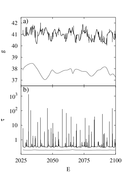
Figure 2 shows the dimensionless conductance and the Wigner-Smith time delay [in units of ] for parameters corresponding to a mixed phase space (, ) and a chaotic phase space with no apparent stability island (, ) for transmitting modes. The differences are quite dramatic. For the fully chaotic case, both quantities are smooth functions of energy and in good agreement with semiclassical theory (see below). While the average values are comparable, many sharp isolated resonances on top of a smooth background are visible in the mixed case [16], also in contrast to the semiclassically predicted fractional Brownian motion. The simple explanation that these narrow resonances are related to quantum tunneling into the islands of regular motion [17] does not apply here, as the phase space volume of stable islands is about 5%, while the narrow resonances (below the mean level spacing) make up about 18% of all states associated with the billiard. This roughly corresponds to the phase space volume around the stable islands where trapping of chaotic trajectories occurs.
In order to analyze the narrow resonances in the mixed case, it is convenient to examine the Wigner-Smith time delay. Each resonance in the time delay has the Breit-Wigner shape, characterized by a width and a height situated at an energy on top of a smooth background. We find our data well described by
| (2) |
with . Since the phase shift through a resonance is , width and height are related by . The energy was initially sampled on an equidistant grid and subsequently refined in order to resolve the sharp resonances. Only resonances with a , i.e. much smaller than the initial grid are lost. As a result we can numerically construct the cumulative distribution of resonance widths, corresponding to the probability of finding a resonance smaller than (Fig. 3). The distribution is very broad, spanning 5 orders of magnitude, and is approximately a power law , with , over a wide range below the mean level spacing .

The consequences of this broad distribution of resonance widths for the variances of conductance and time delay increments are studied now. For correlations between different isolated resonances () do not contribute to the variance , which then is governed by the distribution of resonance widths. Each resonance is reflected in the conductance,
| (3) |
where is a function of the width and the typical height . is the number of resonances with in the energy interval over which we take the average. The variance of the increments of a single resonance is given by
which defines and where is a numerical factor of order unity. Since the distribution of widths is very broad, the strong inequalities are almost always fulfilled in the sum over resonances. Splitting this sum into resonances smaller and larger than , we get
| (7) |
Replacing the sums by integrals over the density of widths and neglecting the weak fluctuations of and as compared to , we can estimate for small ,
| (8) |
where stands for the average over isolated resonances. A power law distribution of resonances thus leads to a power law increase of the variance of conductance increments with the exponent given by .
Fig. 4 a) shows the variances of the conductance increments. On scales smaller than the minimum resonance width the variance increases quadratically, as expected. On larger scales we find the power law Eq. (8). This result coincides with the semiclassically derived Eq. (1) with , however, only on scales below the mean level spacing. At present, there is no explanation why the classical exponent appears on such small energy scales. Remarkably, on scales above the mean level spacing the correlation energy for the conductance fluctuations is given by the Weisskopf width , as in the fully chaotic case (see below).
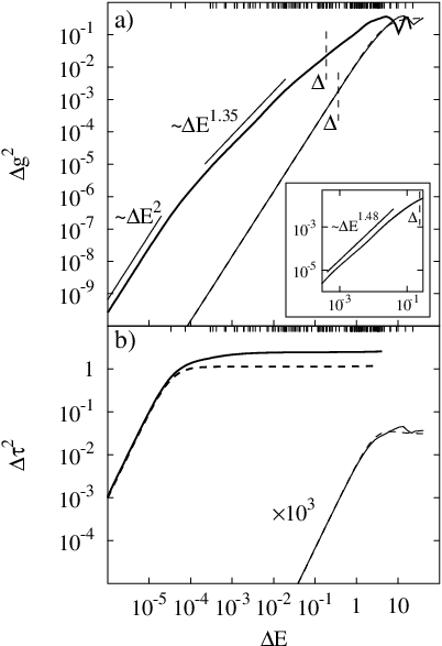
The variance of increments of the time delay are shown in Fig. 4 b). Since the variance measures the square of the resonance peak height in the time delay, in the mixed case, they are completely dominated by the sharpest resonance, once the energy exceeds the minimum resonance width. Thus, in contrast to fully chaotic systems, in mixed systems the scale of the correlations of the time delay is the smallest resonance width and not the Weisskopf width .
For comparison in Fig. 4 we also show the results for and for the fully chaotic case. They are characterized by single scales and and are in good agreement with semiclassical results [4, 19]. The chaotic case can also be described by the random matrix theory (RMT) [20], whose results coincide with the cited semiclassical ones for [21]. In the absence of direct processes, random matrix theory predicts a single correlation scale, known as Weisskopf correlation width, , where the sum runs over all channels with transmission probability [22]. Approximating by twice the average dimensionless conductance we obtain , in agreement with the numerical values within the statistical accuracy. Before concluding, it is worthwhile to stress that depending on and the coupling to the leads, quantum chaotic scattering can also exhibit isolated resonances. Their width distribution, however, follows a -distribution with degrees of freedom [20], rather than power law.
In conclusion, we have shown that generic Hamiltonian systems, which have regular as well as chaotic phase space regions, differ drastically in the Landauer conductance and Wigner time delay from fully chaotic systems. We find many isolated narrow resonances with a power law distribution of their widths accompanied by a power law increase of the variance of conductance increments. Both power laws appear to be connected to the classical power law trapping, surprisingly they only appear on scales below the mean level spacing. Similar unexplained power laws are found in recent studies using quantum graphs [23] modeling a mixed phase space (see inset of Fig. 4 a) [18]. Further research on the quantum signatures of classically mixed systems is urgently needed.
R.K. thanks I. Guarneri for many stimulating discussions. We thank L. Hufnagel, F. Steinbach, and M. Weiss for the inset of Fig. 4 a). This work was supported by the DFG and the ITP at UCSB (B.H.), CNPq and PRONEX (C.H.L.), and the ICTP in Trieste (B.H and C.H.L.).
Note added.—The authors of Ref. [18] have informed us that there are quantum graphs where the classical and quantum exponents do not agree.
References
- [1] Present address: Institut für theoretische Physik III, Ruhr-Universität Bochum, D-44780 Bochum, Germany
- [2] L. P. Kouwenhoven et al., in Mesoscopic Electronic Transport edited by L. P. Kouwenhoven, G. Schön, and L. L. Sohn (Kluwer, Dordrecht, 1997)
- [3] C. M. Marcus, R. M. Westervelt, P. F. Hopkins, and A. C. Gossard, Chaos 3, 643 (1993); A. Chang, H. U. Baranger, L. N. Pfeifer, and K. W. West, Phys. Rev. Lett. 73, 2111 (1994).
- [4] H. U. Baranger, R. A. Jalabert, and A. D. Stone, Chaos 3, 665 (1993).
- [5] L. Markus and K. Meyer, Generic Hamiltonian Dynamical Systems are neither Integrable nor Chaotic, No. 114 in Mem. Amer. Math. Soc. (American Mathematical Society, Providence, Rhode Island, 1974).
- [6] A.J. Lichtenberg and M.A. Liebermann, Regular and Chaotic Dynamics (Springer-Verlag, New York, 1992).
- [7] B.V. Chirikov and D.L. Shepelyansky, Phys. Rev. Lett. 82, 528 (1999); and references therein.
- [8] R. Ketzmerick, Phys. Rev. B 54, 10841 (1996).
- [9] This is equivalent to a decaying correlation , as derived (with an error of 1 in the exponent) by Y.-C. Lai, R. Blümel, E. Ott, and C. Grebogi, Phys. Rev. Lett. 68, 3491 (1992).
- [10] In fact, it deviates somewhat earlier, as analyzed by G. Casati, G. Maspero, and D.L. Shepelyansky, Phys. Rev. Lett. 82, 524 (1999).
- [11] H. Hegger et al., Phys. Rev. Lett. 77, 3855 (1996).
- [12] A. S. Sachrajda et al., Phys. Rev. Lett. 80, 1948 (1998).
- [13] G. Casati, I. Guarneri, and G. Maspero, Phys. Rev. Lett. 84, 63 (2000).
- [14] G. A. Luna-Acosta et al., Phys. Rev. B 54, 11410 (1996); A. Bäcker, R. Schubert, and P. Stifter, J. Phys. A: Math. Gen. 30, 6783 (1997); and references therein.
- [15] F. A. Maaø, I. Zozulenko, and E. Hauge, Phys. Rev. B 50, 17320 (1994).
- [16] Such isolated sharp resonances were also found in kicked systems with a mixed phase space coupled to perfect leads by I. Guarneri et al., private communication.
- [17] P. Šeba, Phys. Rev. E 47, 3870 (1993).
- [18] R. Ketzmerick, L. Hufnagel, F. Steinbach, and M. Weiss, to be published.
- [19] B. Eckhardt, Chaos 3, 613 (1993).
- [20] T. Guhr, A. Müller-Groeling, and H. A. Weidenmüller, Phys. Rep. 299, 189 (1998).
- [21] N. Lehmann et al., Physica 86D, 572 (1995).
- [22] C. H. Lewenkopf and H. A. Weidenmüller, Ann. Phys. 212, 53 (1991).
- [23] T. Kottos and U. Smilansky, Phys. Rev. Lett. 79, 4794 (1997).