[
Conductances, Conductance Fluctuations, and Level Statistics on the Surface of Multilayer Quantum Hall States
Abstract
The transport properties on the two-dimensional surface of coupled multilayer heterostructures are studied in the integer quantum Hall states. We emphasize the criticality of the surface state and the phase coherent transport properties in the thermodynamic limit. A new, stable numerical algorithm for large scale conductance calculations in the transfer matrix approach is discussed in detail. It is then applied to a directed network model describing the quantum mechanical tunneling and impurity scattering of the multilayer edge states. We calculate the two-probe conductance in the direction parallel to the external magnetic field, its fluctuations and statistical distributions as a function of the interlayer tunneling strength. Using finite size scaling, the asymptotic scaling functions of the ensemble averaged conductance and the conductance fluctuations are calculated for a fixed aspect ratio and found to be in remarkable agreement with the analytical results obtained using the supersymmetric nonlinear -model approach. The conductance distribution is determined in the quasi-one-dimensional metallic, insulating, as well as the crossover regime where comparisons are made to that at the single-layer quantum Hall transition. We present, for the first time, a detailed study of the level statistics in the eigenvalue spectrum of the transfer matrix. Coexistence of metallic and insulating statistics is observed in the crossover regime, which is attributed to the emergence of a finite range level repulsion in the crossover regime, separating the metallic (Wigner-surmise) behavior at small level spacings from the insulating (uncorrelated or Poisson) behavior at large level spacings.
pacs
PACS numbers: 73.20.Dx, 73.40.Hm, 73.33.-b, 72.15.Rn, 05.30.-d.]
I Introduction
When a two-dimensional electron gas (2DEG) is placed under a strong perpendicular magnetic field, it exhibits a remarkable set of low-temperature magnetotransport behaviors known as the quantum Hall effect (QHE) [1, 2, 3]. The main part of the phenomenology can be summarized by the existence of (1) new stable phases of matter, i.e. the quantum Hall states, with vanishing dissipation and quantized Hall conductances; (2) continuous, zero temperature phase transitions between the quantum Hall states; and (3) extended, current-carrying, edge states in the quantum Hall liquids. These edge states are intrinsically chiral due to the complete breaking of time reversal symmetry by the external magnetic field.
Two-dimensionality has been regarded as a necessary condition for observing the QHE. Recently, the question concerning what happens to the physics, e.g. the three aspects mentioned above, associated with the QHE in materials having engineering dimensions between two and three has received substantial theoretical and experimental interests. Integer quantized Hall plateaus have been observed experimentally in weakly coupled 30 [4] and 200 [5] multilayer GaAs/AlGaAs graded structures. In the presence of finite interlayer tunnelings, the latter are the natural generalizations of the QHE above 2D. There are several important issues [6, 7, 8]: (1) the quantization condition for the Hall resistance; (2) the stable phases of matter and the nature of the phase transitions; (3) the new physics associated with the edge states phenomena in the quantum Hall states.

In this paper, we shall focus on (3), under the condition that the multilayer graded heterostructure is in the bulk quantum Hall state. In this case, the bulk localization length is finite and very short. The edge state in each layer thus decouples from the bulk. New physics arises because the finite interlayer tunnelings on the sample boundaries couple the edge states supported by individual layers together to form an interesting 2D system on the surface of the multilayer [6, 7]. This is shown schematically in Fig. 1. At this stage, one assumes that the electron-electron interactions can be ignored and the edge states can be treated as independent electrons undergoing impurity scattering and interlayer tunneling as described in Fig. 1.
The three most noteworthy novelties of the surface state under such settings are as follows. (i) It is a 2D chiral system because of the unidirectional edge states. (ii) As such, the backscattering mechanism of 2D weak localization is effectively suppressed. The surface electrons are in a critical state, in the sense that the localization length is linearly proportional to the linear dimension of the surface [6]. (iii) The transport is intrinsically anisotropic. Let us consider such a sample surface as shown in Fig. 1, with dimensions in the interlayer direction and a layer circumference . In the presence of disorder, the chiral nature of the edge states keeps the in-plane transport ballistic with a velocity . The typical time required for an electron to circumnavigate the sample is thus given by a ballistic time . The transport along the direction parallel to the magnetic field (-direction) becomes, on the other hand, diffusive characterized by a diffusion constant which is controlled by the strength of the interlayer tunneling . This leads to a diffusion time across the sample in the -direction.

The transport property in the magnetic field direction () has been a recent subject of considerable theoretical [6, 7, 9, 10, 11, 12, 13, 14] and experimental interests [15]. The most striking feature is the emergence of several regimes of phase coherent transport in samples where the phase coherent length . These regions are most clearly exhibited in the plane spanned by and the surface aspect ratio,
| (1) |
as shown schematically in Fig. 2. (1) The localization length of the critical state, , separates the metallic regime for from the quasi-1D insulating regime for . This crossover is shown by the horizontal line at in Fig. 2, where . (2) Next, equating the ballistic time and the diffusion time leads to a new length scale . Associated with the latter is another crossover between a chiral 2D and the quasi-1D metallic regime, as shown in Fig. 2 by the curved line with on which . In the 2D metal regime, the electrons typically diffuse across before ballisticly traverse across the circumference . (3) Finally, the regime of small and large is expected to be dominated by ballistic transport.
For fixed dimensions and , and thus fixed aspect ratio , the conductance in the -direction is expected to show smooth crossovers between the three regimes as a function of the interlayer tunneling . Alternatively, for a fixed , the crossovers take place with varying sample geometry. The dashed line in Fig. 2 shows an example of the latter, along which is kept fixed. As increases and sweeps through and , transport properties cross over from those of a 2D chiral metal to those of the quasi-1D metal and finally to those of a quasi-1D insulator.
In this work, we are interested in the transport properties along the field direction in the thermodynamic limit, i.e. when and . A large scale numerical transfer matrix algorithm will be discussed and applied to calculate the two-terminal conductance and its mesoscopic fluctuations in phase coherent samples. The behaviors in the thermodynamic limit will be obtained via finite size scaling. Note that the transport behaviors of the surface state in the thermodynamic limit depend crucially on how the latter is taken. In particular, since , the thermodynamic state reached along a path with a finite but fixed aspect ratio corresponds, for any interlayer tunnelings, to the 1D metallic or insulating regimes, where , as shown in Fig. 2. The 2D chiral metallic regime, on the other hand, can only be reached in the thermodynamic limit with a vanishing aspect ratio (see Fig. 2) and . The scaling forms for the ensemble averaged conductance and its variance have been written down by Gruzberg, Read, and Sachdev (GRS) [13, 14],
| (2) |
and similarly, the -th central moment follows,
| (3) |
Here, the crossover lengths and depend on and the strength of the interlayer tunneling . Note that the scaling variable , with being the localization length in a finite system, contains the aspect ratio () dependence in the scaling limit where [16].
In the quasi-1D regime, it was pointed out by GRS that the scaling functions and should follow those in a quasi-1D wire [13, 14]. The asymptotic forms of the latter have been obtained exactly by Mirlin et al. using the supersymmetric nonlinear -model [17]. The exact scaling functions in the chiral 2D regime are not known. Recently, they have been studied perturbatively, and the leading order corrections to the scaling function have been obtained [14]. The first comparison of numerical calculations with these analytical results was made by Cho, Balents, and Fisher [28]. In addition to study the behaviors of the mean conductance and its variance, we will also analyze the behaviors of the conductance distribution function and the level statistics in different regimes and near the crossover.
The rest of the paper is organized as follows. In section II, we will describe a directed network model for transport on the surface. We will discuss the properties of the transfer matrix for chiral transport and compare it to the one used in the 2D quantum Hall transport. In section III, we will discuss a new numerical algorithm for large scale conductance calculations. The method for studying the level statistics is also explained. We will then present our numerical results in section IV and conclude in section V together with a discussion of the open issues.
II Directed Network Model
To facilitate a calculation of the transport properties in the presence of a smooth-varying impurity potential, we model the motion of the electrons on the surface (see Fig. 1) by the directed network (DN) model shown in Fig. 3 introduced by Chalker and Dohmen [6, 18]. The propagation of the chiral edge states is represented by the directed links in the DN. The impurity scattering is accounted for by letting the wavefunctions accumulate random Aharonov-Bohm phases along the links [19]. The interlayer tunneling between the edge states take place at the nodes of the DN.

We define the dimensions of the DN in Fig. 3 as follows: along the horizontal () direction, corresponding to columns of nodes where tunneling between adjacent layers takes place among the coupled layers; in the transverse () direction, which amounts to a layer circumference of rows of nodes. For simplicity, the lattice constants of the DN will be set to unity such that and are dimensionless numbers. Periodic boundary conditions are applied in the transverse direction, whereas two semi-infinite ideal leads will be attached to the ends for the calculation of the two-terminal conductance in the -direction.
The difference of the DN from the Chalker-Coddington network model for the integer quantum Hall transport [19] is that the probability current on all the links is unidirectional. As a result, the structure of the transfer matrix describing a quantum tunneling event at a node is different. As shown in Fig. 3, at each node, there are two incoming and two outgoing modes. Let us denote the associated probability amplitudes by , , , and . The transfer matrix must be defined in a way such that the transfer process is multiplicative throughout the DN,
| (4) |
where is a transfer matrix. The current conservation at each node implies that must leave invariant, i.e.,
Thus, has noncompact unitary symmetry, . With a choice of gauge, one has,
| (5) |
controlled by a real tunneling parameter . Notice that , i.e. for the chiral surface transport, belongs to the noncompact unitary group with determinant negative unity. In general, is determined by the Fermi energy and the local potential. We will take to be the same on all the nodes, corresponding to uniform interlayer tunnelings. We found that a randomly distributed about a finite mean value across the DN is irrelevant for the asymptotic transport properties of the critical surface states. This situation is reminiscent of the one encountered in the ordinary network model description of the integer quantum Hall transition [19]. In the latter case, the randomness in the tunneling amplitude at the saddle [ points of the random potential was found to be irrelevant [20, 21].
The scattering -matrix, on the other hand, transforms the incoming amplitudes to the outgoing ones at a node,
| (6) |
where and are the transmission and the reflection coefficients respectively. From Eqs (4) and (5), one finds,
| (7) |
In the rest of the paper, we will study the transport properties as a function of the single-node interlayer tunneling strength .
It is instructive to compare the transfer matrix in Eq. (5) to the one describing the quantum Hall transport within the layer [19],
| (8) |
The transfer matrix in this case belongs to the noncompact unitary group with determinant . Thus, the two problems are very different and belong to different ensembles of random matrices, except in the pathological limit of , i.e. and , where .
Using Eq. (5) as the building block, one can construct the transfer matrix for the -th column of the DN in Fig. 3,
| (9) |
Here are the random U(1) phases on the links of the DN. The transfer matrix for the -th column has a slightly different structure,
| (10) |
for periodic boundary conditions. Here
are again the random U(1) phases.
]
The total transfer matrix for the entire DN is given by the matrix product,
| (11) |
Correspondingly, the scattering -matrix has the form
| (12) |
where and are the transmission and reflection matrices respectively.
Now we discuss the symmetry properties of the transfer matrix product in Eq. (11). The current conservation across the entire DN implies that must leave
Thus forms a noncompact unitary group that has the following metric preserving properties:
| (13) | |||||
| (14) |
where the matrix can be written as a direct product (),
of the Pauli matrix and the identity matrix . Notice the minus sign in Eqs (13) and (14). This is a consequence of defining the transfer matrix that is multiplicative across the DN, as in the single-node case in Eq. (4). As a result, , i.e. the noncompact unitary group is not volume-preserving.
What we will show next is that the relevant hermitian matrix entering the conductance formula (see section III) has the desired properties. Substituting Eq. (14) to the left hand side of Eq. (13) for leads to,
| (15) |
Thus, forms the volume-preserving U(C,C) group. Denoting the eigenvalues of the latter by , , in descending order, , we next show that the eigenvalues form reciprocal pairs,
| (16) |
Under a unitary transformation,
the matrix has the same set of eigenvalues . Following Ref.[22], Eq. (15) implies that
| (17) |
With the following choice of ,
the metric preserved by in Eq. (17) becomes
Thus the matrices belong to the symplectic group Sp(C). As a consequence, the eigenvalues of , and thus those of , form reciprocal pairs as in Eq. (16). This property will be used in the conductance calculations in the following section.
III Numerical Algorithm
To determine the two-terminal conductance in the magnetic field direction (), two semi-infinite ideal leads are attached at the left and right ends of the disordered DN in Fig. 3. The conductance is then given by the Landauer formula [23, 24],
| (18) |
where is the transmission matrix defined in Eq. (12). Using the unitarity of and the symplectic property of , it is straightforward to show that Eq. (18) can be written in terms of the transfer matrices [25],
| (19) |
Further simplication can be made by writing the ordered eigenvalues () of as,
| (20) |
Evaluating the trace in Eq. (19) leads to,
| (21) |
In the remainder of the paper, we will set the conductance unit .
The two-terminal conductance can be calculated from Eq. (21) or Eq. (18) for a given sample with a disorder realization. The conductance distribution is then obtained by repeating the calculation for a large ensemble of samples with microscopically different disorder realizations. The ensemble averaged conductance, conductance fluctuations, and in fact all statistical properties of the conductance can be obtained from the conductance distribution. Nevertheless, this conceptually straightforward procedure has been hindered by the numerical difficulties involved in evaluating the product of a large number of random transfer matrices (see e.g. Eq. (11)). Unlike the localization length, which can be obtained in the quasi-1D limit of a long stripe or a cylinder using Oseledec’s theorem [26], the conductance of a sample requires the knowledge of the product matrix of random transfer matrices of dimension (Eq. (19)), or equivalently, that of all its eigenvalues (Eq. (21)). For large and , direct calculation of the product is impossible as one quickly looses numerical stability in multiplying the transfer matrices due to the inevitable dynamical range problem. The latter refers to the inability of today’s computers to keep within accuracy of exponentially growing and exponentially decreasing matrix elements. As a result, the applicability of this method has been limited to small system sizes.
Now we discuss a stable numerical algorithm that removes the above difficulty. We shall first prove a theorem, which is then applied to the evaluation of the eigenvalues in Eq. (21).
Consider a general hermitian matrix with non-degenerate eigenvalues.
Theorem 1 The -th power of , i.e. the matrix can be written in the form:
| (22) |
where, in the limit of large , (i) is a unitary matrix of which the columns converge to the eigenvectors of ; (ii) is a diagonal matrix and the eigenvalues of is given by in descending order; (iii) is a right triangular matrix with unity on the diagonals that converges to a limiting matrix of that structure.
Proof: Let us begin with the fact that the hermitian matrix can be factorized according to,
| (23) |
This UDR-decomposition is identical to the well-known Gram-Schmidt procedure for orthonormalizing the column vectors in . Apply to Eq. (23), one has,
| (24) |
Here we have done another UDR-decomposition to the product . Thus is right triangular with unit diagonal elements. Now we interchange and ,
| (25) |
where is right-triangular with non-vanishing elements,
| (26) |
Thus Eq. (24) becomes,
| (27) |
where
| (28) |
are diagonal and right-triangular matrices respectively. Repeating the steps from Eq. (23) to Eq. (27) leads to
| (29) |
and the following recursion relations,
| (30) | |||||
| (31) |
Eq. (29) is a matrix-factorized form of the product matrix . The unitary matrix is necessarily well conditioned. We will show below that the right-triangular matrix is well defined and converges to a limiting matrix of that structure exponentially fast with increasing . The large variations in the size of the matrix elements, which limit the dynamical range of the matrix multiplications, are contained solely in the elements of the diagonal matrix . In fact the Gram-Schmidt orthonormalization procedure ensures that, in the limit of large , the columns of the unitary matrix project onto the eigenvectors of .
Next, we demonstrate the convergence of and obtain the eigenvalues of . The important point is that, in each step, the UDR-decomposition is done by orthonormalizing the -th column with respect to all columns of index . As a result, the diagonal elements of are accumulated in descending order, i.e. for . Carrying out one more multiplication,
| (32) |
Interchanging with ,
| (33) |
where
| (34) |
Since is nonzero for , Eq. (34) shows that the off diagonal elements () are suppressed exponentially with increasing by the ratio of , while the diagonal elements remain to be unity. Thus, when is large, approaches the identity matrix provided that there is no degenerate elements in . The convergence of the matrix follows since for large . Going back to Eq. (32), we have
| (35) |
Using the fact that , Eq. (35) implies,
| (36) |
Thus we have proven that for large , the eigenvalues of is given in descending order by the diagonal matrix , and the columns of the unitary matrices and converge to the corresponding eigenvectors. In the absence of nearly degenerate eigenvalues, the procedure converges exponentially fast, such that in practice need not be too large to obtain the desired accuracy.
It is straightforward to construct an algorithm for evaluating the eigenvalues of the transfer matrix product in the conductance Eq. (21) following the steps of the proof described above. Specifically, we consider as defined by
| (37) |
The eigenvalues of is obtained by the above UDR-decomposition of
| (38) |
In practice, the UDR-decomposition need not be performed after every
multiplication, as this is the most time-consuming part of the
computation. It scales at best with , .
The number of possible direct multiplications without losing accuracy,
, depends on the size of the matrix elements in , thus the
tunneling parameter , and weakly on the size of the matrices.
Algorithm:
- 1.
Carry out steps of direct matrix multiplications in Eq. (38).
- 2.
Perform a UDR-decomposition as described above.
- 3.
Repeat the above procedure for a total of multiplications for the convergence of the factorized matrices.
- 4.
For the last multiplications, store and accumulate the logarithm of the elements in the diagonal matrix for each of the UDR-decompositions as
(39) For large enough , gives the set of eigenvalues for in descending order.
- 5.
To check convergence, apply again to the unitary matrix at the end of the last UDR-decomposition. Repeating step 4, one has
(40) The difference between and can be compared to the convergence criterion, and thus determine the appropriate power .
- 6.
The conductance can be readily calculated from Eq. (21).
We emphasize that the applicability of this stable algorithm for conductance calculations is very general. It is particularly useful for studying phase-coherent transport properties in disordered macroscopic and mesoscopic systems in the thermodynamic limit. The only limitation in this case is the CPU time. It has been successfully applied to study the conductance and conductance fluctuations in the 2D integer QHE [21, 27]. The specific choice of the two parameters, and , depends on the system under investigation (see section IV). In general, it is more convenient to choose such that is an integer. Otherwise, an additional UDR decomposition must be performed at the end of each set of the multiplications. As evidenced in the procedure leading to the proof of the above algorithm, essentially, only and need to be kept, and can be discarded in each of the UDR decomposition. Thus, even the standard Gram-Schmidt procedure works for the present purposes. In the next section, we will apply this technique to study the statistical properties of the transport on the surface of a layered quantum Hall state.
IV The Quasi-1D Regime
To study the quantum interference effects in the conductance, it is convenient to introduce the Ohmic conductance in the classical limit, . The latter can be obtained analytically for the DN in Fig.3 by summing over all possible non-crossing Feynman paths contributing to the -axis transport, while ignoring the nontrivial interference effects associated with the intersecting ones winding at least once around the circumference of the DN [6, 28]. This leads to the averaged conductance,
| (41) |
where is the interlayer tunneling amplitude defined in Eq. (7). The -dependence in the denominator in Eq. (41) is indicative of the ballistic contribution that dominates in samples with . Thus, the crossover from ballistic to diffusive transport is rather slow if is close to one.
In the limit , one recovers the Ohmic behavior in the -direction from Eq. (41),
| (42) |
As a result, the dependence of measurable quantities on the microscopic parameter can be favorably replaced by the dependence on the Ohmic conductance or the conductivity . For example, as discussed in Refs [9, 13, 14], the 1D to 2D crossover length in the scaling equations (2) and (3) can be expressed as
| (43) |
and the localization length as
| (44) |
We consider square DNs with aspect ratio , unless otherwise specified. The asymptotic behavior of the transport properties in the thermodynamic limit taken with will be determined using the finite size scaling (FSS) analysis. In this case,
| (45) |
such that the system is always in the quasi-1D regime in the thermodynamic limit (see Fig. 2). In fact, this is true so long as the latter is taken with a fixed finite aspect ratio, . Nevertheless,
| (46) |
which allows one to study the crossover between the quasi-1D metallic () and insulating () regimes as a function of the interlayer tunneling in the thermodynamic limit.
A Conductances and Conductance Fluctuations
For a given disorder realization, we calculate the conductance from the Landauer-formula in the form of Eq. (21) using the algorithm described in the last section. Next the conductances of a large ensemble containing to microscopically different samples are calculated. This is done for a sequence of sample sizes of to to facilitate the FSS analysis. The typical parameters used are the following. The direct number of multiplications ranges from for large (approaching one from below) to for small (approaching zero). The power is typically less than which is more than enough to suppress the systematic errors in the obtained eigenvalues below the statistical errors associated with ensemble averaging. The latter is typically less than for our data.
We first present the results for the ensemble averaged conductance. In the quasi-1D regime, the scaling function in Eq. (2) becomes, in the asymptotic limit,
| (47) |
For fixed aspect ratio, Eq. (46) shows that is only a function of .
As an example, the calculated is shown in Fig. 4 as a function of at or , which is in the metallic regime. The apparent size dependence is due to the corrections to scaling. To extract the asymptotic value, we perform a FSS analysis according to,
| (48) |
where is the dimension of the leading irrelevant operator that controls the corrections to scaling and is a non-universal constant introduced by the conjugate finite length scale.

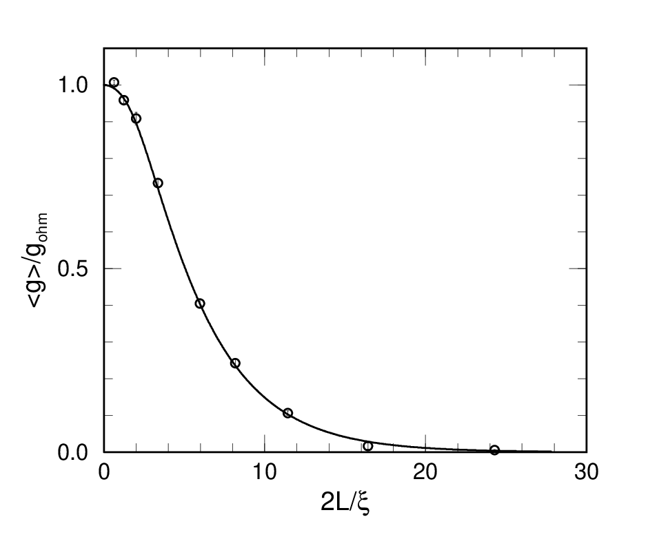
Following this procedure, the asymptotic values of the conductance are obtained for different values of . In Fig. 5, the conductance normalized by the Ohmic value, , is plotted as a function of in accordance with Eq. (47). The solid line is the analytical scaling function obtained by Mirlin et al. for a quasi-1D wire using the supersymmetric non-linear -model [17]. The agreement throughout the entire regime is remarkable, which is in accordance with the analytical work of GSR [13]. It is important to note that such an excellent agreement can only be obtained for the conductances in the thermodynamic limit by the FSS analysis of large sample sizes. In fact, the nature of the finite size corrections is quite different on the metallic and the insulating side of the crossover. Let us define
| (49) |
One finds that as consistent with the fact that the system is critical for all [6]. However, we find that there exists a well defined tunneling amplitude, , such that for , whereas for . It is thus natural to associate the existence of with a sharp crossover from the metallic to the insulating regime. The corresponding crossover conductivity is and . These observations provide an explanation of the systematic deviations from the analytical curve observed numerically in relatively small systems [28].
Next we present the results for conductance fluctuations about the ensemble-averaged values. Once again, we observe significant size dependence in the variance of the conductances. The latter is indicative of the fact that the universality of these conductance fluctuations is a property of the quantum transport at criticality [21, 27, 14], and is outside the context of the conventional universal conductance fluctuations in diffusive metals [29]. Eq. (3) has now the asymptotic form,
| (50) |
The asymptotic values of the variance are plotted in Fig. 6 as a function of to display the scaling function in Eq. (50). The solid line is the analytical result of obtained by Mirlin et al. [17]. As in the case of the ensemble-averaged conductance, the agreement for the asymptotic variance of the conductance is excellent for the entire quasi-1D regime.
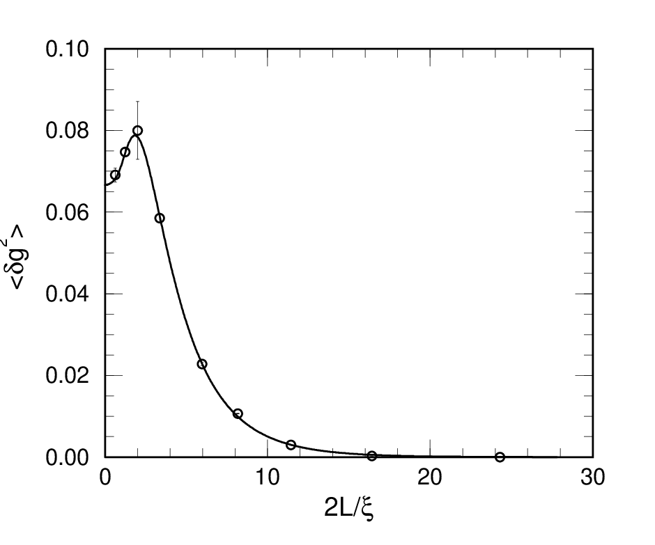
In the limit of small , the asymptotic variance approaches the universal value , despite the vanishingly small fluctuations at small where the transport is ballistic. In the opposite limit of large , the system is in the 1D insulating regime where the absolute fluctuations decay exponentially. Nevertheless, it is important to note that in the insulating regime,the averaged conductance itself decays exponentially [17],
| (51) |
and it is therefore not meaningful to focus on the absolute values of the variance. In fact, a well known result is that the relative fluctuations are exponentially large,
| (52) |
deep in the quasi-1D insulating regime.
We emphasize that this is the first time that conductances and conductance fluctuations are numerically evaluated in the thermodynamic limit in this quasi-1D regime. The agreement between the numerical data obtained from the DN model and the analytical results from the supersymmetric nonlinear -model is, as far as we know, unprecedented.
B Higher Moments and Conductance Distributions
Next, we present the results for the conductance distributions in different regimes and provide a statistical description of the distribution functions, . This will be done by focusing on (1) the largest square samples we have studied, i.e. DNs, (2) three values of , , and that are typical representations of the metallic, crossover, and insulating regimes.
(i) In the metallic regime, the distribution of the conductance for samples is shown in Fig. 7. The solid line is a fit to the Gaussian distribution
| (53) |
The central-moments, , are computed for up to from the data and compared to those determined by the Gaussian fit in Eq. (53). The good agreement shows that the conductances are close to being normal distributed in the metallic regime. The deviation at large values of from the Gaussian moments observable in Fig. (8) is indicative of the log-normal tails in the conductance distribution function [31].


(ii) In the insulating regime, we plot the distribution of the logarithm of the conductance in Fig. 9 obtained from samples. Here the solid line is a fit to the log-normal distribution,
| (54) |
The higher central-moments obtained from our data and the fitted log-normal distribution are compared in Fig. 10.

The excellent agreement confirms that the conductance follows a log-normal distribution in the quasi-1D insulating regime. Thus, instead of the conductance, it is the logarithm of the conductance that is a self-averaging quantity.

(iii) It is important to ask how the statistical distribution changes in the crossover regime from the metallic and insulating behaviors. In this case, we focus on and . The conductances of a large ensemble of samples were calculated to achieve better statistics. The conductance distribution, , is plotted in Fig. 11. Remarkably, the conductance is broadly distributed between and , analogous to the behavior of found in the Chalker-Coddington network model at the critical point of the integer quantum Hall transition [21, 27, 30]. The -th order central-moments are shown in Fig. 12 up to , which can be very well fitted by
| (55) |
with .


Since Eq. (55) is indicative of a distribution with log-normal tails [31], in Fig. 13, we plot the distribution of the logarithm of the conductance, . The latter turns out to show a skewed log-normal distribution as a result of the sharp fall off of close to . The conductance can be described surprisingly well by a log-normal distribution as shown by the solid line in Fig. 13.

We point out the interesting similarity between the above features in the crossover regime (iii) and those found at the 2D integer quantum Hall transitions [21, 27]. A possible scenario to explain this is the following. The critical properties of the quantum Hall transition are described by those of the Chalker-Coddington (CC) network model at criticality [19, 20, 32]. As pointed out in Refs [32, 21], there exists a critical manifold, corresponding to a line of fixed points, for the CC network model that has the same tunneling parameter at each node (see Eq. (8)). One can show that, as the tunneling parameter is varied along this line, the critical conductance exhibits a crossover from 2D metallic to quasi-1D insulating behaviors [33]. The conventionally studied quantum Hall transition corresponds to a particular point on the critical line selected by requiring an additional degrees rotational invariance of the network. The latter happens to be in the crossover regime with [20] and . It is possible that the distribution of the conductance at the critical point in the regime of crossover between metallic and insulating behaviors possesses the universal features that have been observed in both of the systems discussed above.
C Level Statistics
It is well known that the difference in the statistical properties of the conductance in disordered metals and insulators originates from that of the statistical distribution of the eigenstates. A natural quantity to study is the distribution of the normalized (by the averaged value) energy level spacings, often called the level statistics. Traditionally, one applies the random matrix theory developed by Wigner to study the level spacing distribution of an ensemble of random Hamiltonian matrices [34]. More recently, it has become clear, by the Coulomb gas analogy and the maximum entropy hypothesis [22, 35], that the same theory describes the level statistics of the eigenvalues of the transfer matrix. The latter, in contrast to those of the Hamiltonian matrix, correspond to the scattering eigenstates and are directly related to the Landauer formulation of the conductance by Eq. (21).
Here we present our analysis of the transfer matrix level statistic in the quasi-1D metallic, insulating, and the crossover regimes of the multilayer quantum Hall surface states. Following Eq. (20), let us introduce the normalized eigenvalues for a given sample,
| (56) |
The normalized level spacing between adjacent eigenvalues is given by,
| (57) |
where is the averaged level spacing,
| (58) |
According to the random matrix theory, the behavior of the level distribution, , is determined by the level correlations. In the metallic phase with extended eigenstates, the level repulsion is strong and long-ranged, follows the Wigner hypothesis,
| (59) |
with . In the unitary universality class, , and and from normalization. On the other hand, in the insulating regime with exponentially localized states, the levels are uncorrelated, the asymptotic behavior of for large follows the Poisson distribution,
| (60) |
where is a positive constant. However, the behavior of at the critical point of metal-insulator transitions, or in the crossover regime between metals and insulators is an unresolved issue under active current debate [36, 37, 38, 39, 40].
From the set of the calculated eigenvalues , we now study the properties of the distribution . Notice that in general, the eigenvalue distribution is not uniform. In order to obtain a meaningful , one has to, as is normally done [41, 39, 40], unfold the spectrum of according to
| (61) |
such that the distribution is uniform. The level spacings are then obtained by replacing with in Eq. (56).
In Fig. 14, the typical in the quasi-1D metallic region is shown for . The solid line is a fit to the Wigner-surmise in Eq. (59) with , , in very good agreement with the values expected for the unitary universality class. The small discrepancy of from may be attributed to insufficient statistics at small and finite size effects.

The level statistics becomes more intricate in the crossover regime. In Fig. 15, we show at . The most interesting feature is the coexistence of metallic-like and insulating-like statistics. The Wigner-surmise in Eq. (59), with and , remains a rather good description (solid-line) of the data so long as is not too large. On the other hand, the tail at large is clearly described by Poisson statistics as shown by the dotted line. The two different statistics merge together around . This kind of hybrid of metallic and insulating behaviors was first pointed out by Shklovskii, et. al. to describe the level statistics at the 3D Anderson metal-insulator transition [36, 37]. These results suggest that, in the crossover between the metallic and insulating regimes, the level correlation becomes finite-ranged, which manifests itself in the crossover of from the correlated Wigner-surmise statistics to the uncorrelated Poisson statistics at large . Interestingly, such behaviors are also observed at the integer quantum Hall transitions [27], suggesting that the results of Shklovskii, et. al. may be valid for all delocalization transitions. Analogous to the conductance distribution discussed above, this is likely to be a general property of the critical eigenstates.

The distribution of the level spacings in the insulating regime is shown in Fig. 16 for . As expected, the region of the uncorrelated Poisson tail at large expands as a result of the reduction of the correlation range of the levels. This can be seen by comparing Fig. 15 with Fig. 16 at large . One expects to eventually follow the Poisson distribution deep in the insulating regime, i.e. for . It is interesting to point out that the coexistence of metallic and insulating-like statistics is very robust and extends over a wide range of values.

V Summary and Discussions
In conclusion, we have studied the transport properties of the chiral edge states on the surface of a multilayer integer quantum Hall state in the field direction. We emphasized the criticality of the surface state, and that different behaviors of coherent transport can be reached depending on the path along which the thermodynamic limit is taken. The sample aspect ratio is an important quantity that enters the scaling function of the conductance and conductance fluctuations. We presented in detail a new and stable algorithm for large scale conductance calculations in the transfer matrix approach to the Landauer formulation. This algorithm allowed, for the first time, a FFS analysis of the conductance and conductance fluctuations in the thermodynamic limit of the DN model of the chiral surface state. The transport properties, in the thermodynamic limit approached with a fixed aspect ratio, resemble that of a quasi-1D conductor, showing a smooth crossover between metallic and insulating behaviors as a function of the interlayer tunneling. The asymptotic scaling function of conductance and its variance are found to be in remarkable agreement with the analytical functions obtained using the supersymmetric nonlinear -model [17]. The statistics of the two-terminal conductance is found to follow the normal distribution in the metallic and log-normal distribution in the insulating regime. In the crossover regime, the conductance is broadly distributed between zero and , which is well described by a highly skewed log-normal distribution, similar to that found at the 2D quantum Hall transitions [21]. We also presented, for the first time, a detailed study of the level statistics in the eigenvalue spectrum of the transfer matrix. While the latter in the metallic regime follows the Wigner-surmise in the unitary universality class, coexistence of correlated metallic and uncorrelated Poisson statistics characteristic of an insulating state is found to describe the data in the crossover regime. We interpret the latter as a manifestation of the finite range nature of the level correlations, which emerges in the crossover to the insulating regime.
Finally, we briefly discuss the transport behaviors in the 2D metallic regime (see Fig. 2). As discussed below Eq. (3), in the thermodynamic limit, the 2D chiral metal survives only in systems with a vanishing aspect ratio. The behavior of the conductance and conductance fluctuations can be obtained through FSS of a sequence of samples with aspect ratio and . For example, one can approach the asymptotic limit with , where is a constant. Eqs (43) and (44) would then lead to and . The scaling equations for the conductance and conductance fluctuations in Eqs (2) and (3) become, in the asymptotic limit,
| (62) | |||||
| (63) |
It would be interesting to compare results obtained this way with the perturbative spin-wave expansion results derived by mapping the problem to a 1D Su(n,n) quantum ferromagnetic spin chain in the limit [14]. However, in the DN model, because the ballistic contribution dominates at large (), in order to probe the asymptotic 2D regime of vanishing aspect ratio, one has to go to much larger system sizes [28]. The stable algorithm present here makes it feasible to carry out such numerical calculations. These results will be discussed in a future publication [33].
VI Acknowledgments
The authors would like to thank Božidar Jovanović for many useful discussions. They acknowledge useful conversations with Jan Engelbrecht, Ilya Gruzberg, Dung-Hai Lee, Nick Read, and Subir Sachdev, and helpful correspondence with Boris Shklovskii. This work is supported in part by an award from Research Corporation and the IHRP (500/5011) at the National High Magnetic Field Laboratory.
References
- [1] K. von Klitzing, G. Dorda and M. Pepper, Phys. Rev. Lett. 45 494 (1980).
- [2] D. C. Tsui, H. L. Störmer, and A. C. Gossard, Phys. Rev. Lett. 48, 1559 (1982).
- [3] The Quantum Hall Effect, R. E. Prange and S. M. Girvin eds. 2nd Editions, (Springer-Verlag, 1990); Perspectives in Quantum Hall Effects: Novel Quantum Liquids in Low-Dimensional Semiconductor Structures, S. Das Sarma and A. Pinczuk, eds. (Wiley, 1996).
- [4] H. L. Störmer et al, Phys. Rev. Lett. 56, 85 (1986).
- [5] J. S. Brooks, et al., to be published.
- [6] J. T. Chalker and A. Dohmen, Phys. Rev. Lett. 75, 4496 (1995).
- [7] L. Balents and M. P. A. Fisher, Phys. Rev. Lett. 76, 2782 (1996).
- [8] Z. Wang, Phys. Rev. Lett. 79, 4002 (1997).
- [9] L. Balents, M. P. A. Fisher, and M. R. Zirnbauer, Nucl. Phys. B 483, 601 (1996).
- [10] Y. B. Kim, Phys. Rev. B53, 16420 (1996).
- [11] H. Mathur, Phys. Rev. Lett. 78, 2429 (1997).
- [12] Y.-K. Yu, Report No. cond-mat/9611137, (1996).
- [13] I. A. Gruzberg, N. Read, and S. Sachdev, Phys. Rev. B55, 10593 (1997).
- [14] Ilya A. Gruzberg, N. Read, and S. Sachdev, Report No. cond-mat/9704032, (1997).
- [15] D. P. Druist, P. J. Turley, K. D. Maranowski, E. G. Gwinn, and A. C. Gossard, Phys. Rev. Lett. 80, 365 (1998).
- [16] We thank I. A. Gruzberg, N. Read, and S. Sachdev for clarifying this point to us.
- [17] A. D. Mirlin, A. Muller-Groeling, and M. R. Zirnbauer, Ann. Phys. 236, 325 (1994).
- [18] L. Saul, M. Karda, and N. Read, Phys. Rev. A 45, 8859 (1992).
- [19] J. T. Chalker and P. D. Coddington, J. Phys. C 21, 2665 (1988).
- [20] D-H Lee, Z. Wang, and S. A. Kivelson, Phys. Rev. Lett. 70, 4130 (1993).
- [21] Z. Wang, B. Jovanović, and D-H Lee, Phys. Rev. Lett. 77, 4426 (1996).
- [22] K. A. Muttalib, J.-L. Pichard, and A. D. Stone, Phys. Rev. Lett. 59, 2475 (1987).
- [23] D. S. Fisher and P. A. Lee, Phys. Rev. B23, 6851, (1981).
- [24] H. U. Baranger and A. D. Stone, Phys. Rev. B40, 8169 (1989).
- [25] J.-L. Pichard and G. André, Europhys. Lett. 2, 477 (1986); Y. Imry, Europhys. Lett. 1, 249 (1986).
- [26] V. I. Oseledec, Trans. Mosc. Math. Soc. 19, 197 (1968).
- [27] B. Jovanović and Z. Wang, to be published.
- [28] S. Cho, L. Balents, and M. P. A. Fisher, Report No. cond-mat/9708038 (1997).
- [29] P. A. Lee and A. D. Stone, Phys. Rev. Lett. 55, 1622 (1985); P. A. Lee, A. D. Stone, and H. Fukuyama, Phys. Rev. B35, 1039 (1987).
- [30] S. Cho and M. P. A. Fisher, Phys. Rev. B55, 1637 (1997).
- [31] B. L. Al’tshuler, V. E. Kravtsov, and I. V. Lerner, Phys. Lett. A134, 488 (1989); JETP Lett. 43, 441 (1986); Sov. Phys. JETP 64, 1352 (1986).
- [32] D-H Lee and Z. Wang, Phil. Mag. Lett. 73, 145 (1996); and to be published.
- [33] V. Plerou and Z. Wang, to be published.
- [34] M. L. Mehta, Random Matrices, 2nd edition, (Academic Press, Boston, 1991).
- [35] J.-L. Pichard, N. Zanon, Y. Imry, and A. D. Stone, J. Phys (Paris) 51, 587 (1990).
- [36] B. I. Shklovskii, B. Shapiro, B. R. Sears, P. Lambrianides, and H. B. Shore, Phys. Rev. B47, 11487 (1993).
- [37] I. K. Zharekeshev and B. Kramer, Phys. Rev. Lett. 79, 717 (1997).
- [38] A. G. Aronov, V. E. Kravtsov, and I. V. Lerner, JETP Lett. 59, 39 (1994).
- [39] Y. Ono, H. Kuwano, K. Slevin, T. Ohtsuki, and B. Kramer, J. Phys. Soc. Jpn. 62, 2762 (1993); T. Ohtsuki and Y. Ono, J. Phys. Soc. Jpn. 64, 4088 (1995).
- [40] T. Kawarabayashi, T. Ohtsuki, K. Slevin, and Y. Ono, Phys. Rev. Lett. 77, 3593 (1996).
- [41] J.-L. Pichard, in Quantum Coherence in Mesoscopic Systems, edited by B. Kramer, pp. 369-400, (Plenum Press, New York, 1991).