Correlation functions of one-dimensional anyonic fluids
Abstract
A universal description of correlation functions of one-dimensional anyonic gapless systems in the low-momentum regime is presented. We point out a number of interesting features, including universal oscillating terms with frequency proportional to the statistical parameter and beating effects close to the fermion points. The results are applied to the one-dimensional anyonic Lieb-Liniger model and checked against the exact results in the impenetrable limit.
One of the most striking results of modern physics is that in three spatial dimensions particles are either bosons or fermions, i.e. the wave-function of identical objects is either symmetrical or antisymmetrical under the permutations of space coordinates. Conversely, in lower dimensions generalized anyonic statistics, with intermediate properties between bosons and fermions are possible anyons. Fractional braiding statistics in two dimensions are considered a key ingredient to describe fractional quantum Hall effect, motivating the large scientific effort to understand two dimensional generalized statistics. In one dimension (1D) collision is the only way to exchange particles and consequently statistics and interaction are inextricably related. This is the main reason why in 1D we can use bosonization and fermionization (Jordan-Wigner) to attack complicated problems that in higher dimensions are intractable. Excitations in 1D fluids can then experience generalized statistics (not necessarily anyonic ges). However only recently a systematic study of interacting 1D anyonic systems started for different physical motivations. First transport in quantum Hall fluids is localized on the edges and it is due to 1D (chiral) anyons (see e.g. Fradkin). Second recent experiments in ultra-cold atoms succeeded in confining essentially 1D interacting systems 1datoms and there is a proposal in this field to observe fractional statistics paredes. However a general treatment of correlation functions of interacting anyonic systems was still missing. In this letter we fill this gap giving a universal description of low-energy correlation functions in 1D anyonic fluids.
Anyonic statistics are described in terms of fields that at different points () satisfy
| (1) | |||||
where for and . is called statistical parameter and equals for bosons and for fermions. Other values of give rise to general anyonic statistics “interpolating” between the two familiar ones.
In 1D there is a natural way of defining an anyonic field in terms of a bosonic one Kundu: , where , i.e. anyonic and bosonic density are the same (there is also a construction in terms of fermionic field Girardeau that will not be exploited in this letter). It is straightforward to show that if satisfies usual bosonic commutation relations, then follows Eqs. (1). In this letter we establish the behavior of correlation functions of anyonic gapless systems (quantum fluids) in the low energy regime following the original idea of Haldane Haldane for standard statistics (here we closely follow the notations of the review Cazalilla). The starting point is to split , where refers to the slow parts (i.e. it consists of the fluctuations over distances ) and stands for the remaining “fast” modes. On a physical basis it is natural to replace in the definition of the anyonic field with , since fast fluctuations cancel in the integral. Then one can define the operator via and the previously introduced anyonic field becomes
| (2) |
while the density is Haldane; Cazalilla. In the bosonization (or equivalently conformal filed theory) language it is useful to introduce the operators and via and which satisfy the commutation relation . An alternative (constructive) approach would have been to start from these definitions of and and show that the field in Eq. (2) satisfy anyonic statistics Eqs. (1), however we think that this way of introducing the anyonic field is more pedagogical.
All correlation functions in the low momentum regime can be obtained in terms of the so called vertex operators
| (3) |
For example, in terms of these operators it is straightforward to show that when the one-body density matrix (i.e. the Fourier transform of the momentum distribution function) admits the expansion
| (4) |
that holds for all cyclic boundary conditions (the multiplicative factor is determined only in terms of the high energy structure and it is not universal). However to proceed we need to fix the boundary conditions (BC). For simplicity, we now fix the bosonic field to satisfy periodic BC, obtaining (for a proof see e.g. Haldane; Cazalilla)
| (5) |
that lead to the main result of this letter
| (6) |
Here , are unknown non-universal amplitudes that can be eventually fixed only through the exact/numerical computation of correlation functions in the specific model (as e.g. done for the XXZ spin chain lt and for the Bose gas ccs using completely different approaches). The exponent is instead universal and can be written as . and are phenomenological parameters (with the dimensions of velocity) introduced by Haldane to fully characterize the low-energy behavior of a quantum fluid Haldane. They correspond to density and phase stiffness respectively. In practice they must be extracted from the solution of the model (when available), from numerics or, ultimately, from experimental data. In terms of these parameters, the velocity of the sound (i.e. the real speed of excitations in the interacting system) is . For systems with Galilean invariance it holds , where is the Fermi velocity of a gas of spinless fermions with density , and consequently .
Let us briefly discuss the role played by the BC. Fixing periodic ones for the field (and also for ) implies that satisfy twisted BC . Requiring periodic BC for leads to properly chosen twisted BC for . Lack of space prevents us to show all these possibilities, but we note that when equals an even integer the two conditions are equivalent. The appropriate BC for a given physical situation can be quite specific and depend on electrical and magnetic properties of anyons (see e.g. the example in Ref. AB). It is also easy to generalize the bosonic results of Ref. Cazalilla with open BC and at finite temperature to the present case. Asymptotic different times correlations can be obtained as well. Note that, being the anyonic density equal to the bosonic one, the density-density correlation function coincides with Eq. (61) in Ref. Cazalilla (obviously with fixed by the anyonic dynamic). All these applications of the present method will appear elsewhere prep.
Let us now discuss our finding in the thermodynamic limit . The sum Eq. (6) is dominated by the smallest power law in the denominator. For this is always at , and for large enough systems we can neglect all the terms with . This results in a universal oscillating term whose frequency is a direct measure of the statistical parameter. Conversely for fermions with the terms at and display the same power law (and also, by symmetry, ). Consequently, for close to we expect beating effects due to two oscillations with very close frequency and practically the same amplitude. The relevance of this effect will be explicitely showed later on.
Before considering specific applications, we make a last comment. The definitions of anyonic fields (1) have a periodicity in of period . However this is reflected in a periodicity of the system only if the dynamics (dictated by some Hamiltonian) has the same period. In our approach this is encoded in the exponent giving the real -periodicity (e.g. in the Lieb-Liniger model discussed below the periodicity is Batchelor1).
The previous derivation is completely general and holds for any interacting 1D anyonic fluid. To show the predictive power of this analysis we now consider two specific examples: the free gas and the Lieb-Liniger model.
The free anyonic gas. The momentum distribution function of a (more general) gas of free anyons has been studied in the grand-canonical ensamble in Ref. Liguori. Considering only the case defined by Eqs. (1), fixing the chemical potential in terms of the mean-density, and performing a Wick rotation we have
| (7) |
which is consistent with Eq. (6) with and as known from the dispersion relation Liguori.
The Lieb-Liniger anyonic gas. An exactly solvable interacting model is the anyonic Lieb-Liniger gas, defined by the Hamiltonian:
| (8) |
which describe anyons of mass on a ring of length interacting through a local pairwise interaction of strength (in what follow, we fix ). The mean density is . For the model reduces to the bosonic Lieb-Liniger LL, while for just consists of free fermions. For it is equivalent to a gas of impenetrable anyons called Tonks-Girardeau gas Girardeau. As in the bosonic case, the physics just depends on the dimensionless parameter and not on the two parameters separately.
The model is solvable by means of Bethe Ansatz Kundu; Batchelor1; Batchelor2. The Fock space is spanned by a set of Bethe wave functions, each fully determined by a set of rapidities , solutions of the logarithmic Bethe equations (assuming anyonic periodic BC) Batchelor1
| (9) |
in which are a set of integers (half-integers) quantum numbers for odd (even), and is an effective 1D coupling of a bosonic equivalent model Kundu; foot1. If periodic BC are assumed for a corresponding bosonic field, the Bethe equations do not present the term Kundu. Thus, a part from an eventual shift in the momentum, the Bethe equations are the same as the bosonic Lieb-Liniger at coupling : 1D anyons with periodic BC are equivalent to bosons with twisted BC and viceversa, consistently with the previous general analysis.
For periodic BC, following Batchelor1, we observe that any integer value of can be absorbed in the quantum number and only changes the correspondence between states and quantum numbers: , where stands for the integer part. For this reason it is worthy to define , where stands for the non-integer part . It is then trivial to calculate the speed of the sound Batchelor1 , where for periodic (twisted) BC. Consequently . In particular in the Tonks-Girardeau limit we always have . For arbitrary , is not known analytically, but it is very easy to extract it numerically from the solution of the Bethe equations, see e.g. Ref. Cazalilla.
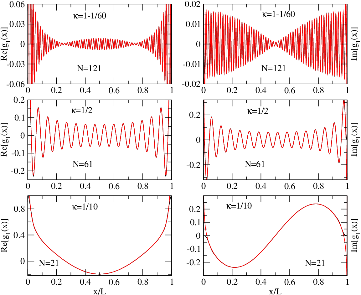
Exploiting the anyon-fermion mapping Santachiara et al. Santachiara gave an exact representation of the one-particle density matrix in the Tonks-Girardeau regime () in terms of the determinant of a Toeplitz matrix for cases when periodic BC are equivalent to twisted BC (i.e. is an integer multiple of ). These exact results must be reproduced by our findings Eq. (6) with . In Fig. 1 we compare the results of Ref. Santachiara with Eq. (6) for the same values of plotted in Ref. Santachiara. For () and () we set and we fix as an overall normalization by imposing the correct value at . The value () is peculiar because very close to the free-fermionic point , where two power-laws () have the same exponents, and all the other . For and the two power laws are still indistinguishable, thus to compare the exact results with Eq. (6) we fix and all the other . The beating effect resulting from two oscillations with almost the same amplitudes is evident as overall nodes (in the amplitude of the fast oscillations) in the real part of at and , in contrast with the monotonic behavior for smaller (see Fig. 1). In the three cases the agreement between exact and asymptotic results is perfect.
Moreover in Ref. Santachiara the asymptotic behavior for large of was estimated using Fisher-Hartwig conjecture. The results obtained in this way are equivalent to the zero mode () in Eq. (6) foot2. On the one hand our results give further evidence that the Fisher-Hartwig conjecture should be valid and is able to fix properly the constant that in our approach remains unknown. On the other hand, Eq. (6) shows that, even for very large , close to the Fermi point the resonance effects cannot be caught by other asymptotic approaches (compare the accuracy of the plot in Fig. 1 for with the analogous one in Ref. Santachiara). However, hard-core anyons are only a specific case to which apply Eq. (6), on the same foot as the Lenard formula Lenard for impenetrable bosons is only the simplest case described by the hydrodynamic treatment of Haldane Haldane for standard statistics.
Discussions. We provided a universal description of correlation functions of 1D anyonic fluids in the low-momentum regime. Our main result is the zero-temperature one-particle density matrix given by Eq. (6). This formula unambiguously shows how to connect smoothly correlations of interacting bosons and fermions through the continuous parameter .
We specifically applied our method to the Lieb-Liniger anyonic gas, but it would be interesting to understand the consequences of our findings in more complicated fluids, as for example a generalized Tomanaga-Luttinger liquid prep, fractional generalization of Heisenberg spin chains as, e.g., the golden chain Feiguin, fluids with internal degrees of freedom (e.g. anyonic extensions of the model in Yang) etc..
We find that the main universal signature of anyonic statistics in the correlation functions is the oscillating complex term that can lead to clear signals in transport experiments Fradkin. The remaining part in Eq. (6) is very similar to the bosonic counterpart Haldane with the generalized statistics leading to a predictable “renormalization” of the power-law behavior for large . This is a manifestation of the 1D interplay between interaction and statistics in the low momentum regime. It would be extremely interesting to understand to which extent some analogous correspondence can be valid for all momenta and in gapped systems.
Acknowledgments. We thank J.-S. Caux, N. Magnoli and R. Santachiara for very fruitful discussions. In particular we are indebted with R. Santachiara and F. Stauffer for providing us numerical data in Ref. Santachiara.
References
- (1) J. Leinaas, J. Myrheim, Nuovo Cimento B 37, 1(1977); F. Wilczek, Phys. Rev. Lett. 48, 1144 (1982).
- (2) F. D. M. Haldane, Phys. Rev. Lett. 67, 937 (1991).
- (3) E.-A. Kim, M. J. Lawler, S. Vishveshwara, E. Fradkin, Phys. Rev. Lett. 95, 176402 (2005); Phys. Rev. B 74, 155324 (2006).
- (4) B. Paredes et al., Nature 429, 277 (2004); T. Kinoshita et al., Science 305, 1125 (2004); T. Kinoshita et al., Nature 440, 900 (2006).
- (5) B. Paredes et al., Phys. Rev. Lett. 87, 10402 (2001).
- (6) A. Kundu, Phys. Rev. Lett. 83, 1275 (1999).
- (7) M. D. Girardeau, Phys. Rev. Lett. 97, 100402 (2006).
- (8) F. D. M. Haldane, Phys. Rev. Lett. 47, 1840 (1981); J. Phys. C 15, 2585 (1981).
- (9) M. A. Cazalilla, J. Phys. B 37, S1 (2004).
- (10) S. Lukyanov, V. Terras, Nucl. Phys. B 654, 323 (2003).
- (11) J.-S. Caux, P. Calabrese, N. A. Slavnov J. Stat. Mech. 0701, P008 (2007) [cond-mat/0611321].
- (12) J.-X Zhu, Z. D. Wang, Phys. Rev. A 53, 600 (1996).
- (13) P. Calabrese, M. Mintchev, in preparation.
- (14) M. T. Batchelor, X. W. Guan, N. Oelkers Phys. Rev. Lett. 96, 210402 (2006); M. T. Batchelor, X. W. Guan, J.-S. He, cond-mat/0611450.
- (15) A. Liguori, M. Mintchev, L. Pilo, Nucl. Phys. B 569, 577 (2000).
- (16) E. H. Lieb and W. Liniger, Phys. Rev. 130, 1605 (1963); E. H. Lieb, Phys. Rev. 130, 1616 (1963).
- (17) M. T. Batchelor, X. W. Guan Phys. Rev. B 74 195121 (2006).
- (18) Note that the low-energy effective treatment of this paper holds only in the region where the effective coupling is positive. In fact, for negative the model possesses bound-states [J. B. McGuire, J. Math. Phys. 5, 622 (1964)] that make the theory gapped and the correlation functions resemble those of a massive field theory [P. Calabrese, J.-S. Caux, cond-mat/0612192].
- (19) R. Santachiara, F. Stauffer, and D. Cabra, cond-mat/0610402.
- (20) An error in the computation of the exponent of was corrected thanks to the comparison with our findings, see v3 of Ref. Santachiara.
- (21) A. Lenard, J. Math. Phys. 5, 930 (1964).
- (22) A. Feiguin et al., cond-mat/0612341.
- (23) C. N. Yang, Phys. Rev. Lett. 19, 1312 (1967).