The critical exponents of the superfluid transition in ⁴He

We simulated the $\phi^{4}$ and ddXY models on simple cubic lattices of size $L^{3}$ with periodic boundary conditions, at several values of the Hamiltonian parameters $\lambda$ and $D$, close to the optimal values $\lambda^{*}$ and $D^{*}$, at which leading scaling corrections vanish. Most of the simulations correspond to $\lambda=2.07$ and $D=1.02$, that represent the best estimates of $\lambda^{*}$ and $D^{*}$ of Ref. CHPRV-01.

The basic algorithm is the same as in our previous numerical study reported in Ref. CHPRV-01. We use a combination of local and clusterWolff-89 updates. We perform wall-cluster updates:HPV-99 we flip all clusters that intersect a plane of the lattice. A cluster update changes only the angle of the variables. An ergodic algorithm is achieved by adding local updates,BT-89 which can also change the length of the spin variables. We use Metropolis and overrelaxation algorithms as local updates, which we alternate with the cluster updates.

The main difference with respect to our previous numerical work CHPRV-01 concerns the random number generator. Since we planned to increase the statistics by approximately one order of magnititude, we decided to use a higher-quality random number generator, such as those proposed in Ref. ranlxd. In our MC simulations we used the ranlux random number generator with luxury level 2. Its main drawback is that it requires much more CPU time than the G05CAF generator of the NAG-library G05CAFgen which we used in Ref. CHPRV-01. In order to get a good performance, despite the use of the expensive random number generator, we used demonized versions Creutz-83; Creutz-92 of the update algorithms, which allowed us to save many random numbers.

Most simulations of the $\phi^{4}$ and ddXY models were performed at the estimates of $\lambda^{*}$ and $D^{*}$ obtained in Ref. CHPRV-01, i.e., $\lambda=2.07$ and $D=1.02$. In addition, we perfomed simulations at $\lambda=1.9,2.1,2.2,2.3$ for the $\phi^{4}$ model, and at $D=0.9,1.2$ for the ddXY model. We shall also present some MC simulations of the standard XY model. In total, the MC simulations took approximately 20 years of CPU-time on a single 2.0 GHz Opteron processor.

The energy density is defined as

The magnetic susceptibility $\chi$ and the correlation length $\xi$ are defined as

and

where

is the Fourier transform of the correlation function at the lowest non-zero momentum.

We also consider several so-called phenomenological couplings, i.e., quantities that, in the critical limit, are invariant under RG transformations. We consider the Binder parameter $U_{4}$ and its sixth-order generalization $U_{6}$, defined as

where $\vec{m}=\frac{1}{V}\,\sum_{x}\vec{\phi}_{x}$ is the magnetization of the system. We also consider the ratio $R_{Z}\equiv Z_{a}/Z_{p}$ of the partition function $Z_{a}$ of a system with antiperiodic boundary conditions in one of the three directions and the partition function $Z_{p}$ of a system with periodic boundary conditions in all directions. Antiperiodic boundary conditions in the first direction are obtained by changing the sign of the term $\vec{\phi}_{x}\cdot\vec{\phi}_{y}$ of the Hamiltonian for links $\left<xy\right>$ that connect the boundaries, i.e., for $x=(L,x_{2},x_{3})$ and $y=(1,x_{2},x_{3})$. Finally, we define the helicity modulus $\Upsilon$. For this purpose we introduce a twisted term in the Hamiltonian. More precisely, we consider the nearest-neighbor sites $(x,y)$ with $x_{1}=L$, $y_{1}=1$, $x_{2}=y_{2}$ and $x_{3}=y_{3}$, and replace the term $\vec{\phi}_{x}\cdot\vec{\phi}_{y}$ in the Hamiltonian with

where $R_{\varphi}$ is a rotation by an angle $\varphi$. The helicity modulus is defined by

The quantities $U_{2j}$, $R_{Z}\equiv Z_{a}/Z_{p}$, $R_{\xi}\equiv\xi/L$, and $R_{\Upsilon}\equiv\Upsilon L$ are invariant under RG transformations in the critical limit. Thus, they can be considered as phenomenological couplings. In the following we will generally refer to them by using the symbol $R$. Finally, we also consider the derivative of the phenomenological couplings with respect to the inverse temperature, i.e.,

which allows us to determine the critical exponent $\nu$ through Eq. (18).

As a first step of the analysis we determine the inverse transition temperature $\beta_{c}$ for various values of $\lambda$ in the $\phi^{4}$ model and of $D$ in the ddXY model. For this purpose we employ the standard Binder-crossing method, i.e., $\beta_{c}$ is determined by requiring

independently of $L$. Here $R$ is a phenomenological coupling, $R^{*}$ is its fixed-point value, and corrections to scaling are ignored. In practice we compute $R(\beta,L)$ as Taylor series up to third order around the simulation value $\beta_{\rm run}$. We choose as $\beta_{\rm run}$ our previous best estimate of $\beta_{c}$, see Ref. CHPRV-01. In the analysis we consider four different phenomenological couplings: $R_{Z}\equiv Z_{a}/Z_{p}$, $R_{\xi}\equiv\xi/L$, $U_{4}$, and $U_{6}$. We do not use the helicity modulus because it has a poor statistical accuracy for large lattices, which are important to determine $\beta_{c}$.

We first analyze the data at $\lambda=2.07$ for the $\phi^{4}$ model and $D=1.02$ for the ddXY model, for which we have data with higher statistics especially for the largest lattices. We perform fits with ansatz (27) for the two models separately. The two models provide consistent results for $R^{*}$, as required by universality. In order to improve the statistical accuracy, we also perform joint fits of the results for both models, imposing the same value of $R^{*}$. We perform fits with various $L_{\rm min}$ and $L_{\rm max}$ (respectively the smallest and largest lattice size taken into account), to check stability. In Table 1 we report our final results, which are taken from joint fits of the results for the two models ($\lambda=2.07$ and $D=1.02$) with $48\leq L\leq 128$. Systematic errors are estimated by comparison with fits with $24\leq L\leq 48$, i.e., by evaluating (difference of the two fits)$/(2^{x}-1)$ with $x=1/\nu+\omega\approx 2.3$ for $\beta_{c}$ and $x=\omega\approx 0.8$ for $R^{*}$ (here we pessimistically assume that leading corrections dominate). The estimates of $\beta_{c}$ obtained by using different quantities are all consistent among each other. As our final result we take the one obtained from the data of $R_{Z}$: $\beta_{c}=0.5093835(2)[3]$ for the $\phi^{4}$ model at $\lambda=2.07$ and $\beta_{c}=0.5637963(2)[2]$ for the ddXY model at $D=1.02$, where the number in parentheses is the statistical error, while the number in brackets is the systematic error due to scaling corrections. In Table 1 we also report the estimates of the fixed-point values $R^{*}$ of the phenomenological couplings, which improve the results of Ref. CHPRV-01. For the other values of $\lambda$ and $D$ considered, we estimate $\beta_{c}$ by requiring that $R(\beta_{c},L=128)=R^{*}$; for $R^{*}$ we use the estimate of $R^{*}$ reported in Table 1. Again, the best estimate is obtained from $R_{Z}$; for this quantity scaling corrections are quite small. The results are reported in Table 2, where the number in parentheses is the statistical error, while the number in brackets is the error due to the uncertainty on $R^{*}$.

Instead of performing the FSS analysis at fixed Hamiltonian parameters, one may analyze the data at a fixed value of a given phenomenological coupling $R$, as discussed in Sec. III. For this purpose we need to compute $R(\beta)$ in a neighborhood of $\beta_{c}$. This could be done by reweighting the MC data obtained in a simulation at $\beta=\beta_{\rm run}\approx\beta_{c}$. However, due to our enormous statistics, we could not store all results needed to reweight the data. Instead, we computed the first derivatives of $R(\beta)$ with respect to $\beta$ and determined $R(\beta)$ by using its third-order Taylor expansion around $\beta_{\rm run}$. We checked that this is by far enough for our purpose. If we do not use the reweighting technique, it is enough to store bin-averages of the different quantities, significantly reducing the amount of needed disk space. Given $R(\beta)$, one determines the value $\beta_{f}$ such that $R(\beta=\beta_{f})=R_{f}$. All interesting observables are then measured at $\beta_{f}$; their errors at fixed $R=R_{f}$ are determined by a standard jackknife analysis. For compatibility with our previous study,CHPRV-01 we choose $R_{Z,f}=0.3202$ and $R_{\xi,f}=0.5925$.

This method has the advantage that it does not require a precise knowledge of the critical value $\beta_{c}$. But there is another nice side effect: for some observables the statistical errors at fixed $R_{f}$ are smaller than those at fixed $\beta$ (close to $\beta_{c}$). This is due to cross-correlations and to a reduction of the effective autocorrelation times. For example, we find

for the ddXY model, with a very small $L$ dependence (within the last figure of the above-reported numbers). In the case of the $\phi^{4}$ model we find slightly smaller improvements for the same quantities. We also mention that the gain is marginal for the derivatives of $R$ considered in this paper. A reduction of the statistical errors when some quantities are measured at a fixed $R$ has also been observed in other models.HPV-05

In order to study corrections to scaling we analyze the value of a phenomenological coupling $R_{1}$ at a fixed value of a second coupling $R_{2}$. If $\beta_{f}$ is determined by $R_{2}(\beta_{f})=R_{2,f}$, we consider

(the dependence on $L$ is understood hereafter). Note that the large-$L$ limit of $\bar{R}_{1}$ is universal but depends on $R_{2,f}$. It differs from the critical value $R_{1}^{*}$, unless $R_{2,f}=R_{2}^{*}$. The phenomenological couplings that we consider are $U_{4}$, $U_{6}$, $R_{Z}\equiv Z_{a}/Z_{p}$, $R_{\xi}\equiv\xi/L$, and $R_{\Upsilon}\equiv\Upsilon L$.

In the $\phi^{4}$ model we define

and analogously for the ddXY model, replacing $\lambda$ with $D$. Since

we perform fits with the most simple ansatz

and analogously for the ddXY model. A selection of such fits is given in Table 3, where we report only results for $\bar{U}_{4}$ and $\bar{R}_{\Upsilon}$ at either a fixed value of $R_{Z}$ or $R_{\xi}$. Using $\bar{U}_{6}$ instead of $\bar{U}_{4}$ leads to very similar results. $\bar{R}_{\xi}$ at a fixed value of $R_{Z}$ is little useful, because the corrections to scaling and the statistical errors are relatively large. In order to get an idea of the corrections to scaling, we give results for the fit intervals $5\leq L\leq 12$ and $10\leq L\leq 24$. The difference of the two results should be a rough estimate of the error due to next-to-leading corrections to scaling. As our final result we quote

which includes (almost) all results for the interval $10\leq L\leq 24$.

To begin with, in Fig. 2 we show results for $\bar{U}_{4}$ and $\bar{R}_{\Upsilon}$ at fixed $R_{Z}=0.3202$, for various values of $\lambda$ in the $\phi^{4}$ model, of $D$ in the ddXY model, and in the standard XY model, vs. $L^{-\omega}$ with $\omega=0.785$. They show a clear evidence of the leading scaling corrections, and of the existence of optimal values $\lambda^{*}$, $D^{*}$ of $\lambda$ and $D$ for which they are suppressed. We also note that $\bar{R}_{\Upsilon}$ is subject to larger next-to-leading scaling corrections; we shall return to this point later.

In order to determine $\lambda^{*}$ and $D^{*}$, we mainly use our data generated for $\lambda=2.07$ and $D=1.02$. We fit them using various ansätze. The most simple one is

where $\bar{R}$ is defined in Eq. (29). Eq. (34) includes only leading corrections to scaling; we fix $\omega=0.785$ as previously obtained. We may also include subleading corrections to scaling and consider

These fits are a bit problematic, since there are several scaling corrections that have similar exponents with $1.8\lesssim\omega_{n}\lesssim 2.0$, see Sec. III. In our fits we use both $\omega_{2}=1.8$ or $\omega_{2}=2$.

We first perform fits of types (34) and (35) for the two models $\phi^{4}$ and ddXY separately. As $\bar{R}$ we consider $\bar{U}_{4}$ at fixed $R_{Z}$, $\bar{U}_{4}$ at fixed $R_{\xi}$, $\bar{U}_{6}$ at fixed $R_{Z}$, $\bar{U}_{6}$ at fixed $R_{\xi}$, and $\bar{R}_{\Upsilon}$ at fixed $R_{Z}$. The results for $\bar{R}^{*}$ are, as required by universality, consistent for the two models. Hence we take our final results from joint fits of the results for both models. For instance, in a joint fit with ansatz (34) there are three free parameters: $\bar{R}^{*}$ and a correction-to-scaling amplitude for each of the $\phi^{4}$ and ddXY models.

In order to determine $\lambda^{*}$ (and analogously $D^{*}$) we assume $c(\lambda)$ to be linear in a neighborhood of $\lambda^{*}$ and write

so that

We use $\lambda=2.07$, the value for which we have most of the simulations, and determine $\mathfrak{c}_{1}$ by using

In the ddXY model we use the same formulas with $D=1.02$ and

In order to determine the needed values of $c(\lambda)$ and $c(D)$, we fix $\omega=0.785$ (and, to estimate errors, $\omega=0.765$, $\omega=0.805$). The results of the fits with ansatz (32) for $\omega=0.785$ are summarized in Table 4. The final estimate is taken from the fits with $12\leq L\leq 24$. The comparison with the fits with $6\leq L\leq 12$ gives us an idea of the error due to subleading corrections. It is small enough to be ignored in the following.

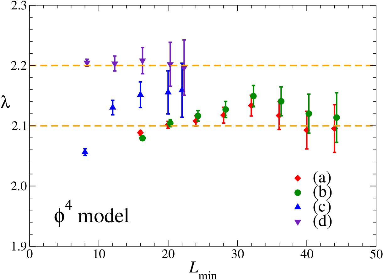
We also checked whether the linear approximation is sufficiently accurate by determining the derivatives (38) and (39) from other pairs of values of $\lambda$ and $D$. The error due to the linear extrapolation is approximately $10\%$, which is negligible for the purpose of determining $\lambda^{*}$ and $D^{*}$. In Fig. 3 we plot the results for $\lambda^{*}$ and $D^{*}$ as functions of the $L_{\rm min}$ used in the fits to (34) and (35). The results of the fits to Eq. (34) show a systematic drift and become stable only for $L_{\rm min}=30$. This systematic variation is mostly due to the next-to-leading corrections and indeed, fits to Eq. (35) are less dependent on $L_{\rm min}$ and give fully consistent results. As our final result we quote

which correspond to

Consistent results for $\lambda^{*}$ and $D^{*}$ are obtained by analyzing $\bar{U}_{6}$ at $R_{Z}=0.3202$ and $\bar{R}_{\xi}=0.5925$. Note that the estimates of $\lambda^{*}$ and $D^{*}$ are slightly larger than those obtained in our previous work,CHPRV-01 where we reported $\lambda^{*}=2.07(5)$ and $D^{*}=1.02(2)$. Since the larger statistics and larger lattice sizes allow us to achieve a better control of all sources of systematic errors, and in particular of the next-to-leading scaling corrections, we are confident that the new estimates (40) are now correct with the quoted errors (that are as large as those reported in our previous work).

We also performed some MC simulations of the standard XY model up to lattice size $L=96$. Using the estimates for $\omega$ and $\bar{U}_{4}^{*}$ obtained above, one-parameter fits of the MC data give (taking data for $24\leq L\leq 96$).

and

We can use these results to obtain a conservative upper bound on the ratios $|c(\lambda=2.15)/c({\rm XY})|$ and $|c(D=1.06)/c({\rm XY})|$ that are independent on the quantity one is considering. Using the estimate of $\partial c/\partial\lambda|_{\lambda=\lambda^{*}}$ and taking into account that the error on $\lambda^{*}$ is $\pm 0.05$, we infer that the leading scaling-correction amplitude of $U_{4}$ at $R_{Z}=0.3202$ for $\lambda=2.15$ satisfies $|c(\lambda=2.15)|<0.0024$. The same bound is obtained in the ddXY model for $c(D=1.06)$. This implies $|c(\lambda=2.15)/c({\rm XY})|<0.0024/0.1014\approx 1/42$ and an analogous bound for $|c(D=1.06)/c({\rm XY})|$. A similar calculation also shows that $|c(\lambda=2.07)|$ and $|c(D=1.02)|$ are at least 20 times smaller than $|c({\rm XY})|$.

In this subsection we present evidence of next-to-leading scaling corrections characterized by an exponent $\omega_{\rm nlo}\approx 2$, as expected due to the presence of several irrelevant perturbations with $y\approx-2$, as discussed in Sec. III. In particular, this provides a robust evidence of the absence of $1/L$ analytic corrections, see discussion at the end of Sec. III.

We first construct improved variables $\bar{U}_{4}|_{R_{Z}=0.3202}$, $\bar{U}_{4}|_{R_{\xi}=0.5925}$, and $\bar{R}_{\Upsilon}|_{R_{Z}=0.3202}$, which do not have leading scaling corrections. In the ddXY model (analogous formulas hold in the $\phi^{4}$ model by replacing $D$ with $\lambda$) we consider

Expanding $\bar{R}$ as in Eq. (34) and using a linear approximation for $c(D)$, $c(D)\approx\mathfrak{c}_{1}(D-D^{*})$, as in the previous section, we obtain for $L\to\infty$

Thus, if we take $x=x^{*}=(D^{*}-D_{2})/(D_{1}-D_{2})$, the leading scaling correction cancels. In the ddXY model we use the data at $D_{1}=1.02$ and $D_{2}=1.2$, while in the $\phi^{4}$ model we combine our data for $\lambda_{1}=1.9$ and $\lambda_{2}=2.3$.

In Fig. 4 we show the improved combination (44) in the case of the Binder cumulant $\bar{U}_{4}$ as a function of $L^{-2}$. For $\bar{U}_{4}|_{R_{\xi}=0.5925}$ we observe straight lines to a good approximation. On the other hand, for $\bar{U}_{4}|_{R_{Z}=0.3202}$ there is a clear bending of the curves, indicating that, in the given range of lattice sizes, corrections with exponent $\omega^{\prime}>2$ are contributing significantly. We should note that these results do not provide a completely independent information, since we have already used $\omega_{2}\approx 2$ as input in the determination of $D^{*}$ and $\lambda^{*}$ in the previous section. Therefore, they only provide a consistency check. This is not the case for $R_{\Upsilon}\equiv\Upsilon L$, since it was not used for the determination of $D^{*}$ and $\lambda^{*}$. In Fig. 4, $\bar{R}_{\Upsilon}|_{R_{Z}=0.3202}$ is plotted as a function of $L^{-2}$. We clearly observe a straight line. Hence corrections with $\omega_{2}\approx 2$ clearly dominate in the whole range of lattice sizes that are shown. There are no leading corrections to scaling and, as expected from general RG arguments, also no corrections proportional to $L^{-1}$. If there were a correction proportional to $L^{-1}$, the ratio of its amplitude with the amplitude of the correction proportional to $L^{-\omega}$ (i.e., the leading one) would not be the same in different quantities. In other words, if corrections proportional to $L^{-1}$ and $L^{-\omega}$ effectively cancel for $U_{4}$ at our estimates of $D^{*},\lambda^{*}$ and for the range of values of $L$ considered, there is no reason why this should also happen for $R_{\Upsilon}$. Hence we conclude that our numerical results confirm the theoretical argument that no $L^{-1}$ corrections are present in FSS for periodic boundary conditions.

References

- (1) J.A. Lipa, D.R. Swanson, J.A. Nissen, T.C.P. Chui, and U.E. Israelsson, Phys. Rev. Lett. 76, 944 (1996).
- (2) J.A. Lipa, D.R. Swanson, J.A. Nissen, Z.K. Geng, P.R. Williamson, D.A. Stricker, T.C.P. Chui, U.E. Israelsson, and M. Larson, Phys. Rev. Lett. 84, 4894 (2000).
- (3) J.A. Lipa, J.A. Nissen, D.A. Stricker, D.R. Swanson, and T.C.P. Chui, Phys. Rev. B 68, 174518 (2003).
- (4) A. Pelissetto and E. Vicari, Phys. Rep. 368, 549 (2002).
- (5) M. Campostrini, M. Hasenbusch, A. Pelissetto, P. Rossi, and E. Vicari, Phys. Rev. B 63, 214503 (2001).
- (6) R. Guida and J. Zinn-Justin, J. Phys. A 31, 8103 (1998).
- (7) J. Zinn-Justin, Quantum Field Theory and Critical Phenomena, fourth edition (Oxford University Press, Oxford, 2002).
- (8) H. Kleinert and V. Schulte-Frohlinde, Critical Properties of Theories (World Scientific, Singapore, 2001).
- (9) M. Hasenbusch and T. Török, J. Phys. A 32, 6361 (1999).
- (10) P. Butera and M. Comi, Phys. Rev. B 60, 6749 (1999).
- (11) M. Campostrini, A. Pelissetto, P. Rossi, and E. Vicari, Phys. Rev. B 61 5905 (2000).
- (12) E. Burovski, J. Machta, N. Prokof’ev, and B. Svistunov, cond-mat/0507352.
- (13) J.A. Lipa, S Wang, J.A. Nissen, and D. Avaloff, Space Advances in Space Research 36, 119 (2005).
- (14) A. Aharony and M.E. Fisher, Phys. Rev. B 27, 4394 (1983).
- (15) J. Salas and A.D. Sokal, J. Stat. Phys. 98, 551 (2000); cond-mat/9904038v1.
- (16) M. Caselle, M. Hasenbusch, A. Pelissetto, and E. Vicari, J. Phys. A 35, 4861 (2002).
- (17) K.E. Newman and E.K. Riedel, Phys. Rev. B 30, 6615 (1984).
- (18) H.G. Ballesteros, L.A. Fernández, V. Martín-Mayor, and A. Muñoz-Sudupe, Phys. Lett. B 441, 330 (1998).
- (19) M. Hasenbusch, K. Pinn and S. Vinti, Phys. Rev. B 59, 11471 (1999).
- (20) M. Hasenbusch, J. Phys. A 32, 4851 (1999).
- (21) M. Campostrini, A. Pelissetto, P. Rossi, and E. Vicari, Phys. Rev. E 65, 066127 (2002); E 60, 3526 (1999).
- (22) M. Hasenbusch, J. Phys. A 34, 8221 (2001).
- (23) M. Campostrini, M. Hasenbusch, A. Pelissetto, P. Rossi, and E. Vicari, Phys. Rev. B 65, 144520 (2002).
- (24) V. Privman, in Finite scaling and Numerical Simulations of Statistical Systems, edited by V. Privman, World Scientific, Singapore, 1990.
- (25) M. Campostrini, A. Pelissetto, P. Rossi, and E. Vicari, Phys. Rev. E 57, 184 (1998).
- (26) S. Caracciolo and A. Pelissetto, Phys. Rev. D 58, 105007 (1998).
- (27) J. Salas, J. Phys. A 35, 1833 (2002).
- (28) N.Sh. Izmailian and C.-H. Hu, Phys. Rev. E 65, 036103 (2002).
- (29) U. Wolff, Phys. Rev. Lett. 62, 361 (1989).
- (30) R.C. Brower and P. Tamayo, Phys. Rev. Lett. 62, 1087 (1989).
- (31) M. Lüscher, Comput. Phys. Commun. 79, 100 (1994).
- (32) The G05CAF generator is a linear congruential generator: with , and .
- (33) M. Creutz, Phys. Rev. Lett. 50, 1411 (1983).
- (34) M. Creutz, Phys. Rev. Lett. 69, 1002 (1992).
- (35) Y.J. Deng, H.W.J. Blöte, M.P. Nightingale, Phys. Rev. E 72, 016128 (2005).
- (36) M. Hasenbusch, A. Pelissetto, and E. Vicari, J. Stat. Mech. P12002 (2005).
- (37) M. Campostrini, J. Stat. Phys. 103, 369 (2001).
- (38) A.J. Guttmann, in Phase Transitions and Critical Phenomena, Vol. 13, edited by C. Domb and J. Lebowitz (Academic Press, New York, 1989).
- (39) D. MacDonald, S. Joseph, D.L. Hunter, L.L. Moseley, N. Jan, and A.J. Guttmann, J. Phys. A 33, 5973 (2000).
- (40) In FT calculations, such as those reported in Ref. GZ-98, one usually introduces the rescaled coupling . Our new estimate of corresponds to , to be compared with the FT result (Ref. GZ-98).
- (41) M. Campostrini, A. Pelissetto, P. Rossi, and E. Vicari, Phys. Rev. B 62, 5843 (2000).
- (42) M. Strösser and V. Dohm, Phys. Rev. E 67, 056115 (2003).
- (43) A. Cucchieri, J. Engels, S. Holtmann, T. Mendes, and T. Schulze, J. Phys. A 35, 6517 (2002).
- (44) Preliminary result, M. Hasenbusch, in preparation.