Mapping Monte Carlo to Langevin dynamics: A Fokker-Planck approachPreprint: APS/123-QED
Abstract
We propose a general method of using the Fokker-Planck equation (FPE) to link the Monte-Carlo (MC) and the Langevin micromagnetic schemes. We derive the drift and diffusion FPE terms corresponding to the MC method and show that it is analytically equivalent to the stochastic Landau-Lifshitz-Gilbert (LLG) equation of Langevin-based micromagnetics. Subsequent results such as the time quantification factor for the Metropolis MC method can be rigorously derived from this mapping equivalence. The validity of the mapping is shown by the close numerical convergence between the MC method and the LLG equation for the case of a single magnetic particle as well as interacting arrays of particles. We also found that our Metropolis MC is accurate for a large range of damping factors , unlike previous time-quantified MC methods which break down at low , where precessional motion dominates.
pacs
75.40.Gb, 75.40.Mg, 75.50.TtWith the rapid advance of computing resources, Monte Carlo (MC) methods have become a powerful tool in many fields ranging from the physical sciences to finance and sociology Landau and Binder 2000; Jaeckel 2002; Stauffer 2003. The flexibility of Monte Carlo is due to its abstract formalism which can be realized in an almost infinite number of ways. Increasingly, MC methods are being implemented in the stochastic micromagnetic modeling of magnetic nanostructures Fidler and Schrefl 2000. Stochastic micromagnetic modeling has important practical implications, e.g. in predicting the storage lifetime of hard-disk magnetic media Néel 1949; Brown 1959. Traditionally, the dynamics of magnetic moments are also modeled in the Langevin scheme, using the stochastic Landau-Lifshitz-Gilbert (LLG) equation Brown 1963. Langevin-based micromagnetics constitutes a formidable computational method, because of its ease of use and close correspondence to actual experimental data in previous literatures Coffey et al. 1998. However, it has certain limitations which may be overcome by MC methods. For instance, MC methods can accommodate the long-time magnetization relaxation dynamics of large-scale arrays of magnetic grains Novotny 1995; Kolesik et al. 1998; Lee et al. 2005, which is practically unfeasible to be modeled using the stochastic LLG equation. On the other hand, MC schemes have the drawback of having its time calibrated in MC steps, instead of physical time units. Thus, both MC and the Langevin approach are useful computational methods in micromagnetics, with complementary strengths and drawbacks. Hence, it is very important to devise a general way of mapping one method to the other, and vice versa.
Early efforts to link MC to LLG were done by Nowak et al. Nowak et al. 2000. They focused on deriving a time quantification factor to relate one MC step (MCS) to real physical time unit used in the LLG equation. Recently, we also proposed another time-quantifiable MC (TQMC) method which involves the determination of macroscopic density of states, and the use of the Master equation for time evolution. This method is applicable in simulating extremely long time magnetization reversal process Cheng et al. 2005. The effect of precession on Nowak’s time-quantification was investigated by Chubykalo et al. Chubykalo et al. 2003. They concluded that Nowak’s time quantification of MC breaks down in the low damping case, in presence of an oblique external field, due to the influence of (athermal) precessional motion.
In this paper, our approach is more thorough and fundamentally different from all previous works. We propose a systematic way of using the Fokker-Planck equation (FPE) to map MC to LLG dynamical equation. The physical background of using FPE to describe stochastic dynamics has been well established Reif 1967, e.g. in the case of a particle under the influence of a one-dimensional potential Kikuchi et al. 1991. The outline of our scheme is as follows. We consider a single isolated particle and then generalize to an interacting array of particles. First, we develop a MC method that has the stochastic dynamics of the LLG equation. This method is a hybrid Metropolis MC scheme which combines the random displacement of spins about a cone and a suitably-sized precessional step. The random displacement models the thermal fluctuation and the precessional step accounts for the precessional term in the LLG equation. From the drift-diffusion picture of the general Fokker-Planck equation, we can then obtain the FP coefficients of this hybrid Metropolis MC method, and compare them with previously obtained FP coefficients of the stochastic LLG equation. The comparison shows an exact equivalence of the two FPEs in the limit of small MC step size. From this comparison, we obtain the time quantification factor to relate one MC step to real time unit and the required step size for the precession, which allows us to map the MC results to that of the LLG equation. Generalization to an array of interacting particles will be shown numerically in the latter part of this paper.
We consider an isolated single domain magnetic particle whose moment can be represented by a Heisenberg spin with an easy axis anisotropy Brown 1963. To describe the dynamics of a Heisenberg spin, it is convenient to use the spherical coordinate system. The FPE in spherical coordinates and can be written in form as:
| (1) | |||||
is the probability density of the moment orientation. and are the so-called drift and diffusion coefficients respectively, defined as the ensemble mean of an infinitesimal change of and with respect to time Risken 1967.
The reduced stochastic LLG dynamical equation can be written as:
| (2) |
where is the magnetic moment unit vector, and are the damping and gyromagnetic constant respectively, is the effective field normalized by the anisotropy field , where is the anisotropy constant, is the magnetic permeability and is the saturation magnetization. The thermal field is introduced by Brown Brown 1963 as a white noise term. The FPE corresponding to the LLG equation has been derived by Brown Brown 1963, and its factors are as follows:
| (3) | |||||
where in above equations, , , , is the total energy Brown 1963; Nowak et al. 2000, is the volume of the particle and , is the Boltzmann constant and is the temperature in Kelvin.
We will now derive the FPE corresponding to our Monte Carlo method. For the MC method, we choose with probability , to displace the magnetic moment within a small cone centered at the original magnetization direction, and with probability to perform a rejection-free precession about an effective field. For the displacement about a cone, we pick a random vector lying within a sphere of radius to the original magnetic moment and then normalize the resulting vector. The precessional step vector, i.e. the displacement of magnetic moment due to precession, is , where is a precesional step size to be determined. The probability is chosen to be , which yields a near-optimal balance of efficiency and accuracy of our simulation.

To calculate the FP coefficient for the MC method, we obtain the ensemble mean of a small change of in one Monte Carlo step. Contributions from random walk and precessional step are , where the angle brackets denote the ensemble average.
We first calculate the , where the angular displacement is defined by two random variables and angle , as shown in Fig. 1. After some geometrical analysis, we obtain:
| (4) | |||||
| (5) |
Next, we require the probability for the displacement vector to be of size and angle with respect to . This probability is given by Nowak et al. Nowak et al. 2000 as . Based on the heat-bath Metropolis MC scheme, the acceptance rate is
| (6) | |||||
where is the energy change in the random walk step. Thus, integrating over the projected surface of Fig. 1, one obtains :
| (7) | |||||
Next we calculate the other contribution from the precessional step :
| (8) | |||||
In the above derivation, we have used the vector identity and . Using Eqs. (7) and (8), becomes,
| (9) |
The other FPE factors can be obtained with the same procedure.
| (10) |
We can now compare the FPE factors corresponding to the Langevin (LLG) equation in Eq. (3), with those of the Metropolis MC method in Eqs. (9) and (10). Performing a term-wise comparison and omitting and higher order terms, we found that there is a one-to-one mapping between all FP terms of MC and LLG if:
| (11) | |||||
| (12) |

Note that is in order of , thus we are justified in neglecting terms in the above comparison between Eq. (3), and Eqs. (9) and (10). From Eq. (11), we obtain the time quantification factor of our hybrid Metropolis MC method, while Eq. (12) determines the precessional step size . After taking into consideration the probability factor , Eqs. (11) and (12) can be reduced to Nowak’s results Nowak et al. 2000 in the high damping case.
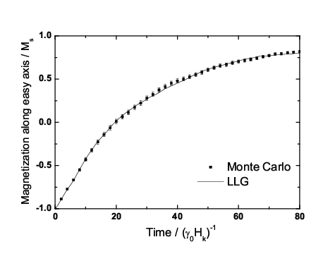
To test the validity of Eqs. (11) and (12), we perform numerical calculations of the switching process for a magnetic particle in which the easy axis is oriented at to the applied field direction. All results are averaged from a few thousand simulations. We consider the time evolution behavior of the mean magnetization component along the easy axis, and found a close convergence between our time-quantified MC method and the LLG equation (Fig. 2). In these calculations, we use for MC, and for the LLG integration. We also apply our analytic results to , and interacting spin array systems. For these simulations, is used. We remark that a smaller step size reduces statistical errors. We obtain a very good convergence between the MC and LLG results for all three arrays (Fig. 3), especially so for the larger arrays. We believe this is due to the effects of self averaging.
Note that our derivation of the FPE factors is applicable in a very general case. For instance, we do not require assumption of the system being in the vicinity of an energy minimum Nowak et al. 2000. The derivation also provides additional information, e.g., it explains mathematically why the Metropolis MC random walk method of Ref. Nowak et al. 2000 fails to include the energy conservative precessional motion. The FPE expression for the pure Metropolis MC does not contain terms corresponding to the -factor related terms of the LLG method [Eq. (3)], which are precisely the terms which reflect the precessional part of the magnetization dynamics Coffey et al. 1996. Thus, as shown in Fig. 4, we have successfully implemented the representation of precessional motion in our MC method. We investigate the influence of damping constant on switching time, where the switching time is defined as the time required for the magnetic moment to reach zero from the initial state. The precessional step size guarantees a precise description of switching process even in the case of very low damping constant , in which precessional motion dominates the reversal process Cheng et al.. By contrast, the results obtained from the pure Metropolis MC method of Nowak et al. diverges significantly from that of the LLG equation at low .

To summarize, we have proposed a general method using FPE to map MC to LLG and vice versa. We derived the drift and diffusion FP terms, corresponding to the MC method and compare them to the FP terms obtained from the LLG dynamical equation. By matching the terms in the drift and diffusion coefficients, we obtain a time quantification factor and the required precessional step size. The idea of using the FPE to link two stochastic methods (MC and Langevin methods) is general, and may be applied to other areas such as molecular dynamics in our future work.
This work was supported by the National University of Singapore Grant No.(R-263-000-329-112). Two of the authors H. K. Lee and Y. Okabe are partly supported by a Grant-in-Aid for Scientific Research from the Japan Society for the Promotion of Science.
References
- Landau and Binder (2000) D. P. Landau and K. Binder, A Guide to Monte Carlo Simulations in Statistical Physics (Cambridge, 2000).
- Jaeckel (2002) P. Jaeckel, Monte Carlo Methods in Finance (John Wiley & Sons, 2002).
- Stauffer (2003) D. Stauffer, Computing in Science and Engineering 5, 71 (2003).
- Fidler and Schrefl (2000) J. Fidler and T. Schrefl, J. Phys. D 33, R135 (2000).
- Néel (1949) L. Néel, Ann Géophys 5, 99 (1949).
- Brown (1959) W. F. Brown, J. Appl. Phys. 30, 130S (1959).
- Brown (1963) W. F. Brown, Phys. Rev. 130, 1677 (1963).
- Coffey et al. (1998) W. T. Coffey, D. S. F. Crothers, J. L. Dormann, Y. P. Kalmykov, E. C. Kennedy, and W. Wernsdorfer, Phys. Rev. Lett. 80, 5655 (1998).
- Novotny (1995) M. A. Novotny, Phys. Rev. Lett. 75, 1424 (1995).
- Kolesik et al. (1998) M. Kolesik, M. A. Novotny, and P. A. Rikvold, Phys. Rev. Lett. 80, 3384 (1998).
- Lee et al. (2005) H. K. Lee, Y. Okabe, X. Z. Cheng, and M. B. A. Jalil, Comp. Phys. Comms. 168, 159 (2005).
- Nowak et al. (2000) U. Nowak, R. W. Chantrell, and E. C. Kennedy, Phys. Rev. Lett. 84, 163 (2000).
- Cheng et al. (2005) X. Z. Cheng, M. B. A. Jalil, H. K. Lee, and Y. Okabe, Phys. Rev. B 72, 094420 (2005).
- Chubykalo et al. (2003) O. Chubykalo, U. Nowak, R. Smirnov-Rueda, M. A. Wongsam, R. W. Chantrell, and J. M. Gonzalez, Phys. Rev. B 67, 064422 (2003).
- Reif (1967) F. Reif, Fundamentals of Statistical and Thermal Physics (McGraw-Hill, New York, 1967).
- Kikuchi et al. (1991) K. Kikuchi, M. Yoshida, T. Maekawa, and H. Watanabe, Chem. Phys. Lett. 185, 335 (1991).
- Risken (1967) H. Risken, The Fokker-Planck Equation (Sprinter-Verlag, Berlin, 1967), 2nd ed.
- Hinzke and Nowak (2000) D. Hinzke and U. Nowak, Phys. Rev. B 61, 6734 (2000).
- Coffey et al. (1996) W. T. Coffey, Y. P. Kalmykov, and J. T. Waldron, The Langevin equation with Applications in Physics, Chemistry and Electrical Engineering (World Scientific, 1996).
- (20) X. Z. Cheng, M. B. A. Jali, H. K. Lee, and Y. Okabe, accepted for publication in J. Appl. Phys.