On the dynamics of the glass transition on Bethe latticesUMR 8549, Unité Mixte de Recherche du Centre National de la Recherche Scientifique et de l’ Ecole Normale Supérieure.
Abstract
The Glauber dynamics of disordered spin models with multi-spin interactions on sparse random graphs (Bethe lattices) is investigated. Such models undergo a dynamical glass transition upon decreasing the temperature or increasing the degree of constrainedness. Our analysis is based upon a detailed study of large scale rearrangements which control the slow dynamics of the system close to the dynamical transition. Particular attention is devoted to the neighborhood of a zero temperature tricritical point.
Both the approach and several key results are conjectured to be valid in a considerably more general context.
pacs
75.50.Lk (Spin glasses), 64.70.Pf (Glass transitions), 89.20.Ff (Computer science)I Introduction
I.1 Motivation
Bethe lattices11 1 We denote by this term random graphs with arbitrary degree distribution (but bounded average degree). A more precise definition is given in Section II for the particular case studied here. can be used to define a large variety of analytically tractable statistical mechanics models. A sophisticated (and still improving) theory has been developed for computing the thermodynamic properties of such systems in great generality (cf. for instance MezardParisiBethe and references therein). Among the recurring predictions of this theory is the occurrence (in models with frustration or self-induced frustration) of a dynamical phase transition (DPT) FranzFerro. While the system free energy remains analytic at the DPT, this is revealed by more refined thermodynamic potentials FranzPotential (such as the configurational entropy) which indicate the appearence of a broken-ergodicity phase.
Despite its eminently dynamical character, the dynamics itself at the DPT is poorly understood. For fully-connected (FC) mean field models, in which each degree of freedom (spin, particle, etc) interacts with all the others, one can usually solve the dynamics in terms of a closed set of equations for the two points correlation and response functions. This is no longer true for models on Bethe lattices, which have finite connectivity (each degree of freedom interacts with a finite number of neighbors). Correlation and response functions involving an arbitrary number of times are relevant in this case SeCuMo. This is somehow healthy: there is no hope to obtain a finite set of closed equations describing the dynamics of realistic (finite-dimensional) systems. Alternative approaches developed for Bethe lattice models may, on the other hand, prove more general.
Consider the relaxation of a particular degree of freedom, for instance a spin. As the DPT is approached, dynamics slows down because, in order for the spin to decorrelate, a larger and larger number of degrees of freedom have to be rearranged coherently. Our approach consists in computing some detailed properties (e.g. their minimal size or the minimal energy barrier to be overcome in order to realize them) of such rearrangements and then using these properties to estimate relaxation times. While we shall develop these ideas on a specific Bethe-lattice model, they are susceptible of generalization to a variety of other examples. The cases of -core percolation and kinetically constrained models RitortReview are, for instance, quite straightforward, and will be treated in a related publication NostroKCM (the model treated in the present paper is in fact strictly related to -core percolation on random hypergraphs).
Due to the lack of a simple order parameter and the extensive configurational entropy, the broken ergodicity phase is often referred to as a “glassy” phase. In the 80’s, Kirkpatrick, Wolynes and Thirumalai KiTh; KiWo stressed the analogy between the DPT (in the context of fully-connected models) and the mode coupling transition MCT; MCA; DynamicsReview, thus motivating a considerable effort aimed at a theoretical understanding of structural glasses. One recent advance has been the definition a “dynamical length scale” associated to the dynamical slowing down Donati; Bennemann. Within mean-field models and mode coupling theory (MCT) this length scale diverges at the DPT FranzChi4A; FranzChi4B; BiroliBouchaud. However, the relation between this phenomenon and the diverging relaxation time is poorly understood. Also, the basic physical mechanism underlying this divergence in glasses is presumably different from the one occurring in simpler system, and is still misterious JPB. Finally, it would be useful to establish a quantitative relation between the dynamical slowing down and some purely static observable.
In order to clarify these points, let us contrast our understanding of the DPT with the one we have of the paramagnetic–to–ferromagnetic transition in the Ising model. In this case a typical configuration close to the transition looks like a patchwork of positively and negatively magnetized regions. The typical linear size of each region is the correlation length , and total magnetization is ( being the susceptibility). Assuming that the magnetization performs a random walk, we can estimate the relaxation time as . Since standard scaling theory predicts , we get . In fact the dynamical scaling hypothesis states that with exponent Halperin.
A further source of motivation is to understand the role of activation at the DPT. Much of our understanding of this phase transition comes from the study of a particular model: the -spin spherical spin glass CrisantiSommers_Statics; CrisantiSommers_Dynamics; Leticia_Houches. MCT has been shown to be exact for this model MCA. Moreover, the energy landscape and its relation to dynamics are relatively simple KurchanTAP. Above the transition temperature, the system never visits minima and moves among saddles. As temperature is lowered the number of energy-decreasing directions decreases, slowing down the dynamics Cavagna. Below the critical point, the system is typically found near a local minimum and is separated by diverging (in the thermodynamic limit) energy barriers from other minima. Activation is therefore irrelevant both above and below the DPT. It is not necessary in the first case, and it cannot take place within physical time-scales in the second. This has lead to question whether activated processes could spoil the predictions of MCT for more realistic (finite-dimensional) models. In this case a standard nucleation argument suggests that ergodicity is restored within a finite (in the thermodynamic limit) time Kob.
Like other mean-field systems, models on Bethe lattices are characterized by diverging energy barriers within the broken ergodicity phase. Therefore, they cannot help understanding the role of activation in this regime. On the other hand, finite energy barriers are present in the ergodic phase and one may ask whether they modify the MCT critical behavior upon approaching the DPT. Notice that such a question is in general not well-defined because the distinction between activated and non-activated processes becomes sharp only in the zero-temperature limit. In the following we shall study in detail a zero-temperature multi-critical point where the distinction makes sense.
I.2 Overview of the paper
The model and some basic notations are introduced in Section II. The phase diagram is described in terms of two basic parameters: the temperature , and which quantify the degree of constrainedness of the system. We then discuss the critical properties of the DPT in Sections III and IV. Let be the phase transition temperature. We will show that -points susceptibilities stay finite at for any given . On the other hand, we introduce a correlation length using point-to-set correlations and show that . This correlation length is connected to relaxation times using a disagreement percolation argument which implies a bound of the form .
We then consider the , finite limit (still within the ergodic phase). In this regime, the dynamics is dominated by activated processes and the relaxation time can be derived from a standard Arrhenius argument. The relevant large scale rearrangements minimize the energy barrier to be overcome in order to realize them, cf. Sec. VI. The barriers height diverges as increases and approach the DPT point (at which ). In Sec. VII, we compute several properties of these rearrangements, such as their size, depth and cooperativity. We also consider minimal size rearrangements (cf. Sec. V), which share several properties with minimal barrier ones, and are somewhat easier to analyze. We compare the critical behavior as with standard MCT predictions. We find that several of these predictions are violated. More surprisingly some universal properties of MCT (such as the divergence of the four point susceptibility) hold even in this extremely activated regime.
The point is a tricritical point, analogous to the percolation point in diluted ferromagnets. In Sec. VIII, we use standard scaling theory in order to connect the , and , regimes. The scaling hypothesis is verified through numerical simulations. Under this hypothesis, temperature is a relevant variable and a crossover from an activation-dominated to a thermal regime takes place. We argue that the thermal regime is controlled by usual MCT critical behavior at any finite temperature.
Some conclusive remarks are put forward in Sec. IX, while most of technical calculations are collected in the Appendices.
A synthetic account of our results was published in Ref. NostroLettera.
II Definitions and notations
II.1 Model
In this paper we focus on Ising models with -spin () interactions:
| (1) |
Here are Ising spins, is a set of -uples of indices, and are quenched couplings taking values with equal probability. The above Hamiltonian is twice the number of violated constraints . Since this condition can be written as the exclusive OR of boolean variables, the problem is known in computer science as XORSAT XOR_CS. Any configuration satisfying all these constraints has zero energy (is unfrustrated).
In order to complete our definition, we need to specify the (hyper)graph of interactions . In this paper we consider to be a random graph constructed by taking the interacting -uples of sites to be quenched random variables uniformly distributed in the set of possible -uples XOR. In the thermodynamic limit , the number of interactions a given spin belongs to (its degree) is a Poisson random variable with parameter . Moreover, the shortest loop through such a spin is (typically) of order with Bollobas.
This property allows (at least in principle) for an exact treatment of the thermodynamics. The phase diagram is sketched in Fig. 1. For and above the critical line the system is ergodic and the free energy density is given by the usual paramagnetic expression . The free energy density remains analytic across the line , but ergodicity is broken in the whole region . Finally, a true thermodynamic transition of the random-first order type KiTh; KiWo takes place at .
Two regimes have attracted particular attention. In the “fully-connected” limit , , both statics and dynamics can be treated analytically, showing a typical MCT transition Gardner; KiTh. The relaxation time diverges as .

In the zero-temperature, finite limit, probabilistic methods can be used to show that zero-energy ground states with finite entropy density exist for . However the set of ground states gets splitted in an exponential number of clusters with extensive Hamming distance (number of spins with different value) separating them for XOR_1; XOR_2. A finite fraction of the spins does not vary among the ground states of a particular cluster, while they change when passing from a cluster to the other. At the fraction of frozen spins jumps from to a finite value . For instance , , and when . This phase transition can be characterized in a purely geometrical way. It corresponds to the appearence of a -core, i.e. a subgraph of such that any of its vertices has degree at least in the subgraph. The largest -core in , denoted as , includes vertices above . The subgraph of frozen spins will be referred to as “backbone”, and can be constructed recursively as follows. Start from , add to it any hyperedge of having at most one vertex not yet in , and repeat until such an hyperedge exist. In view of these remarks, it is not surprising that several results of this paper can be generalized to kinetically constrained models (in this case the relevant geometrical transition is the -core percolation Pittel; RitortReview).
No exact result exists for the dynamics at any finite value of . Standard generating function methods allow to formally derive a hierarchy of dynamical equations for multi-time correlation and response functions SeCuMo. Several approximation schemes have been proposed SemerjianWeigt; CoolenEtAl for this hierarchy. Such approximations have been developed mostly within models with a continuous transition (typically, the model (1) with ). However, their generalization to models undergoing a discontinuous transition is straightforward. Unfortunately such approximations break down in the critical regime .
In the following we shall use repeatedly two useful properties of this model. First: as long as there exist at least one zero-energy ground-state, all such ground-states are equivalent. Suppose that is such a ground state, and that is an equilibrium configuration for the Hamiltonian (1) at temperature . Define (this is often called a “gauge” transformation). Then is distributed according to the Boltzmann measure with an Hamiltonian of the form (1), with the same graph and temperature as the original model, but with for all the interactions (ferromagnetic model). Therefore any property of which is invariant under this change of variable can be computed for the ground state of the ferromagnetic model. In particular, for this implies that the ground states of the model as observed from , “look like” the ground states of the ferromagnetic model as observed from .
The second property will be used uniquely in numerical simulations and can be stated in two parts: As long as does not contain hyperloops (i.e. subgraphs such that each site has even degree) the partition function of the model is exactly given by the annealed computation, i.e. . Under the same hypothesis, sampling the sign of the couplings (for a given graph ) and then the configuration according to the Boltzmann distribution is equivalent to sampling from the uniform distribution and then the couplings as independent random variables with distribution
| (2) |
The proof of this statement is deferred to Appendix A. It is a consequence of the results of Refs. XOR_1; XOR_2 that, for a random graph constructed as above does not contain any hyperloop with high probability.
Sampling first and then is much simpler than the opposite. We shall adopt this procedure in order to generate thermalized configurations for simulating the equilibrium dynamics. It is an open (and interesting) problem whether the same procedure can be useful in the region , (at least for large enough systems).
II.2 Averages, factor graphs and messages
In this paper we shall denote by expectation with respect to the Boltzmann measure at inverse temperature , and by expectation with respect to the quenched disorder (i.e. the graph and the couplings ). Connected correlation functions (see, for instance, ZinnJustin for a definition) are denoted by .
Factor graphs Factor provide an useful representation of models like the one studied in this paper. These graphs have two types of nodes, one for interactions (“function nodes”, squares of Fig. 2) and one for spins (“variable nodes”, circles). Edges connect each interaction with the spins involved in it. The graph is obviously bipartite.
We shall use indices to denote function nodes, and for variables. Directed edges in the graph will support messages of two types, , and , with various meanings depending on the context. We denote by the set of variables in the interaction , and by the set of interactions the variable belongs to. In this context will denote the substraction of an element from a set.

Let be the factor graph associated to the model (1). The degree of function nodes in is fixed to , whereas the one of a generic variable node converges to Poisson random variable of parameter . A path in is a sequence of nodes, such that any two successive nodes are joined by an edge. The distance between two variable nodes and is the length (number of function nodes in it) of the shortest path graph joining them. Two variables are said to be “adjacent” if their distance is equal to one, and connected if there is a path joining them. A set of variables is connected if its elements are pairwise connected. An important property of random graphs, on which we shall come back later, is that, in the limit, any finite neighborhood of a generic site is, with high probability, a tree.
Finally, for asymptotic behaviors (here as ) we write: if is bounded away from and for large enough; if . Further if is numerically close to .
II.3 Glauber dynamics
Most of our results can be applied to general single-spin flip Markov dynamics satisfying the detailed balance condition. Furthermore, the generalization to block (multi-spin flip) dynamics is in several cases straightforward as far as the block size is kept finite as .
For the sake of definiteness, the reader may refer to Glauber dynamics in continuous time. At each spin , a flip is proposed in a time interval with probability (i.e. according to a Poisson process of rate ). Whenever a spin flip is proposed at site , the new value of is drawn from the conditional distribution, given the neighboring spins
| (3) |
(the constant hidden in the symbol is here independent of ). Whenever precise non-asymptotic estimates on correlation times will be given, they will refer to these transition rates.
The basic observables we shall use in order to probe this stochastic dynamics are single spin correlation functions
| (4) |
Here expectation is taken with respect to the equilibrium dynamics, i.e. is an equilibrated configuration, and is the configuration obtained by applying the above dynamics for a time interval . One can also consider the global correlation function , defined by averaging uniformly over the spin position.
III Origin of the dynamical transition
Since purportedly, the dynamics gets slower and slower upon approaching , it is quite natural to think that spatial correlations in the equilibrium measure must become stronger in the same regime. In this Section we first show that -point correlations remain short ranged at the dynamical transition. On the contrary, point-to-set correlations diverge at . We show that this indeed implies a divergence in properly defined relaxation times.
III.1 -points correlation functions
A simple way for characterizing correlations in the system consists in considering -points spin-glass susceptibilities
| (5) |
We are eventually interested in the thermodynamic limit. The rationale for considering the spin-glass susceptibility is that unless and is even 22 2 Whenever contain an index repeated an odd number of times, a simple gauge transformation implies that .. We claim that for any fixed , the susceptibilities (5) remain finite across the dynamic transition . More precisely, for all , with high probability
| (6) |
for some bounded functions . In other words, -points correlation functions give no hint33 3 One may wonder whether derivatives of with respect to (or ) may give some useful information. It is not hard to generalize our arguments to show that this is not the case. about the dynamic transition as far as is finite. Here we will sketch a proof of this claim in the zero-temperature limit (the approach is essentially rigorous in this case) for . Technical calculations, together with a cavity argument for or are presented in Appendix B.
Consider : the system will typically contain an unfrustrated ground state , so we apply a gauge transformation and reduce ourselves to the ferromagnetic model . Since , the definition (5) remains unchanged in the new variables (which we still denote as ). In the ferromagnetic system or for any and . In fact or (for the not-connected correlation function). If in all the ground states then trivially. If on the other hand there exist a ground state such that , this is the case for exactly one half of the ground states (for each ground state with we can construct one of the other type multiplying it by ) and therefore . As for the connected correlation , being sum of products of ordinary correlations, it is an integer. Furthermore, it is non-negative because of Griffiths inequality for , and by simple enumeration of the possible values of , , and so on, for . Using the definition of it is finally easy to show that it cannot be larger than one. We therefore proved the simplified expression
| (7) |
Let with a list of (not necessarily distinct) spin positions denote by the number of unfrustrated ground states such that for any . We take to have Poisson distribution with mean (with ) and i.i.d. uniformly distributed in . Let
| (8) |
denote the ground state entropy of the system in which we forced for any . Simple calculus reveals that
| (9) |
Therefore, proving the thesis for is equivalent to proving that the first two derivatives of are bounded.
By computing derivatives at , one can show that is non-increasing and convex in . Furthermore, since each constraint (either for edge of or for ) at most halves the number of zero-energy ground states, we have the bound . Moreover, it is simple to derive an upper bound through an annealed computation (we refer to Appendix B for the details). Define
| (10) |
where is the binary entropy function. Then one can prove that, given , for any with high probability. It turns out that there exist , with , such that, if ,
| (11) |
For instance we obtain , , for, respectively, . These bounds imply in turn
| (12) |
Thus proving that , , remains bounded for and . In Appendix B, we argue that in fact the result remains true up to .
III.2 Point-to-set correlations
A much stronger criterion for correlations decay is obtained by considering observables depending on arbitrary number of spins (i.e. not necessarily bounded by a constant independent of and as in the previous Section). Here we describe a concrete way for verifying such a criterion and show that it allows to define a correlation length diverging at .
Fix a configuration drawn from the equilibrium Boltzmann distribution at temperature . Let be a site in the system and a positive integer. Consider a configuration distributed according to the Boltzmann measure, conditioned to for all sites whose distance from is at least . In other words, if denotes the subgraph including all the sites at distance smaller than from the distribution of is
If is small, will be highly correlated with . However, we expect this correlation to decay as if the temperature is high enough. We are therefore led to define a correlation length as follows (a similar length scale has been discussed in BiroliBouchaudMosaic)
| (16) |
Here denotes expectation with respect to the reference configuration and is the expectation with respect to the measure . Our definition depends upon the parameter . However this dependency is irrelevant 44 4 The single-site Edwards Anderson order parameter Ricci; Ricci2; ParisiLocal must however be larger than to get a non-trivial result. and we can think of it as a fixed small number e.g. .
The main result of this Section is that diverges as the dynamical transition line is approached. More precisely, with non-vanishing probability –with respect to the choice of the site –, we have (the thermodynamic limit being taken at the outset)
| (17) |
Equivalently, if the dynamical transition is approached by increasing the number of constraints in the system: .
Let us consider, for the sake of simplicity the case and . The finite temperature case will be discussed in App. B (we also refer to Reconstr for a more detailed discussion of this issue). The reference configuration is, for , chosen uniformly at random among the exponentially numerous unfrustrated ground states. Without loss of generality we can assume that the model is ferromagnetic and is the ‘all-plus’ cofiguration. Repeating the type of arguments already used in the previous Section, one can show that, at zero temperature, is either (if is completely determined by the boundary condition together with the requirement of satisfying all the interactions) or (in the opposite case). As a consequence does not depend upon : we have for and for .
Let be the probability that . Obviously . Furthermore, for any , the following recursion relation holds
| (18) |
This formula is proved by summing over the degree of site the probability that the degree is (factor ) times the probability that at least one of the interactions has all the remaining spins determined by their -th neighbors.
The dynamical transition point is given by
| (19) |
Numerical values of are given in Table 1. A simple asymptotic study of the recursion (18) shows that for , while for , being the largest solution of . Hereafter we shall use the notation . For any , and for . As already mentioned, is the critical value for the appearence of a backbone (and a -core) in the graph and is easy to realize that its typical size is about for . In the present picture, the spins in the backbone are frozen because they are determined by spins arbitrarily far away.
 |
 |
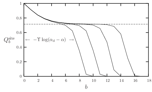
As is approached from below, the convergence of to becomes slower and slower. As can be seen in Fig. 3, first develops a plateau near , whose length scales as and then decreases to right after this plateau (i.e. it decreases below any given constant in a fixed number of iterations). The behavior around the plateau is described by the scaling form
| (20) |
where
| (21) |
and
| (22) |
Therefore, for any given sample, a fraction of the sites is such that
| (23) |
independently of .
 |
 |
To conclude this Section, in Fig. 4 we show the results of a recursive finite- calculation of as a function of , averaged over the graph realization. This allows to extract the typical point-to-set correlation length defined as (here denotes expectation over the graph realization)
| (24) |
Since decreases rapidly to above , it is not hard to argue that with high probability and for a finite fraction of sites/graphs (, being two positive constants). We also plot as a function of the temperature for . As anticipated, the scaling is remarkably well verified allowing for a precise determination of . The approach followed for this computation is described in Appendix B.3.
III.3 Implications for dynamics
As we have seen, at the dynamic transition line , the point-to-set correlation length diverges. It is intuitively clear that this should induce a diverging relaxation time, associated to the (dynamical) glass transition. Imagine for instance to perturb the spin . In order for a new equilibrated configuration (under the perturbed Hamiltonian) to be produced, the effect of the perturbation must propagate over a distance at least of the order of , taking a time at least of order . Therefore yields (up to a finite proportionality constant) a lower bound on the relaxation time for .
Remarkably, this handwaving argument can be turned into a mathematical derivation. For doing this, we need a precise definition for the relaxation time of . We consider the spin autocorrelation function , and define
| (25) |
Notice that is a continuous and non increasing function of (the last property follows from the spectral representation of the Markov dynamics AldousFill). Therefore for any . The precise value of is irrelevant, and it should be thought as a small fixed number. Close to , we expect to develop a plateau. The definition (25) correctly gives the slow time scale for the relaxation of as soon as is smaller than the plateau height, which is in turn equal to the local Edwards Anderson order parameter Ricci; Ricci2.
We also need to introduce a cutoff radius : this is the largest integer such that the subgraph is a tree.
Proposition 1
Assume that , , and that the number of sites at distance from is at most for any and some . Then
| (26) |
Proof: The proof is an application of some probabilistic arguments developed in HayesSinclair; DyerEtAl; BergerEtAl. For greater convenience of the reader, we shall provide a self contained presentation of most of these ideas.
Let be an equilibrium configuration for the system under consideration, an integer and recall the definition of . Consider two Markov trajectories and defined as follows. The initial condition is the same for both processes and is given by the reference configuration : . At times , spin flips are proposed simultaneously in both systems according to the usual Glauber dynamics rule (each spin attempts a flip according to a Poisson process of rate 1). If the spin whose flip is proposed lies outside , the flip is never accepted for , and is accepted according to the usual transition probability for . If, on the other hand, the spin which attempts a flip, let us say , is within , the update is done in the two systems as follows. Let be the probabilities for to take values, respectively, or after the flip. In the case of Glauber dynamics, these are computed according to Eq. (3). Denote by the same transition probabilities for system , and assume, for instance, that . Then, with probability , we set ; with probability , we set and ; finally, with probability , .
Recall that the transition probabilities only depend on the values of the spins on the neighbors of . Therefore, the new values of , will coincide whenever for all the sites at distance one from . Furthermore, it is easy to see that when considered separately, the Markov processes , have a very simple description. The latter is the usual Glauber dynamics with equilibrated initial condition . The former is Glauber dynamics for the subsystem formed by spins in , with initial condition , and boundary condition (outside ) also given by . The joint process is in fact a “Markovian coupling” of these two dynamics.
At , by definition. Since the two dynamics are different outside and will rapidly disagree there. However, inside , disagreement can only propagate at a finite velocity, starting from sites at distance from and moving inward. It is intuitively clear that, in order for the disagreement to reach , a time of order is needed. This intuition can be precised mathematically. Assume and denote by the number of sites at distance from . Then
| (27) |
This inequality is essentially adapted from HayesSinclair, and we refer to this paper for a proof.
We now turn to the main steps of the proof. Using the definition of and the fact that is a non increasing function of , we have
| (28) |
Denote by the indicator function for the event that disagreement did not percolate to up to time . More explicitly
Continuing from the above inequality we get, for ,
| (32) |
Taking , we obtain
| (33) |
Now set 55 5 Here and in the following, denotes the smallest integer greater than or equal to , and the greatest integer smaller than or equal to .. Under the hypothesis of the proposition, and . Therefore
| (34) |
By the definition of , the above equation implies thus proving our claim (using the hypothesis ).
Let us comment on the hypotheses of this Proposition. For a random graph , is, with high probability, close to Bollobas. The hypothesis is therefore satisfied with high probability (although in any given sample there is a vanishing fraction of sites for which this is not the case).
Furthermore, within any fixed distance from , converges to a (Galton-Watson) tree. The number of offspring is a Poisson variable of mean for variable nodes, while it is deterministic and equal to for function nodes. Let the number of -th generation descendants in such a tree. It is easy to show that, for any , with probability approaching one as . On the random graph , the number of neighbors is in fact smaller than on the tree. As a consequence, is finite for most of the sites in the graph and, roughly speaking, of order for a finite fraction of them. On the other hand, can be much larger (diverging as ) for a vanishing fraction of sites. In particular, must be at least as large as the degree of , and the maximal degree in such a random graph scales as .
Finally, the inequality (26) is only interesting in strong correlation regimes, such that . Therefore, the hypothesis does not imply any loss of generality.
In the previous Section we argued that the typical point to set correlation length diverges as upon approaching the glass transition temperature. Therefore we obtained the following lower bound on the typical relaxation time:
| (35) |
As explained below, the usual MCT predictions agree with such a bound.
IV From dynamics to rearrangements
IV.1 On the relaxation time divergence
The inequality (35) –along with its derivation– explicitly shows how a divergent length scale induces a divergent time scale at the (dynamical) glass transition. However, several reasons suggest that this lower bound is not tight. A first indication is provided by the usual predictions of MCT. These imply
| (36) |
with , determined by the equations
| (37) |
and a positive, model-dependent constant between 0 and 1. It is easy to show, using these equations (see also Sec. V), that , and therefore . Although MCT is not exact for the model studied here, we will argue below that several of its predictions are correct (in particular, this can be shown in the fully connected limit KiTh). If this is accepted, it follows that Eq. (35) does not predict the correct critical exponent.
A more fundamental reason for (35) not to be tight is the following. This estimate was derived by showing that a region of linear size requires a time at least of order to relax. This is true because a perturbation propagates at finite speed under Glauber dynamics. However, the time required for equilibration on such a length scale can easily be much larger. Information can for instance propagate by diffusion (leading to ) or equilibration time may be related to the volume rather than to the linear size of highly correlated regions.
In order to understand this point, we shall hereafter focus on the low temperature limit at . In this regime, the system spends most of its time in quasi-ground states, and the leading relaxation mechanisms will be “jumps” from one such low-energy configuration to a different one. Since the properties of these jumps are likely to be continuous with respect to the energy of the starting and arrival points, we shall hereafter assume them to be exact ground states.
The time scale for relaxation of spin can be estimated in this limit through a standard Arrhenius argument. We have , where is the smallest energy to be overcome during a rearrangement of the system which flips (a jump). Due to the definition of our Hamiltonian (1), is an even number. For future convenience we shall write , and refer to the Arrhenius law in the form
| (38) |
We will sometimes call the “barrier” for spin (although, strictly speaking, the energy barrier is ).
A formal definition of rearrangements is given below. While it is clear that energy barriers are the relevant quantities determining time scales in the Arrhenius regime, it is rather involved to evaluate them. For pedagogical reasons we shall at first neglect barriers and look for minimal size rearrangements.
IV.2 Rearrangements
A rearrangement for the site is a set of sites such that belongs to , and for every interaction , an even number of the variables in belongs to . If one starts from a ground state and flips all the spins in , a new ground state is obtained with flipped (viceversa, any two ground states which differ at site , differ in a whole rearrangement ). A rearrangement is “simple” if it is connected and each interaction contains either zero or two sites of . In the following we shall only consider simple rearrangements, and let this restriction understood. It will be clear that, for our purposes (and in particular within the regime) there is no loss of generality in this restriction. denotes the set of all simple rearrangements .
We shall consider observables defined on the set , the simplest one being the number of sites in the rearrangement. Let us discuss the general strategy on this example. The optimal value of the observable , and the set of optimal rearrangements with respect to their size are, respectively,
| (39) |
Unless it diverges with the system size (which can be checked a posteriori), , as well as the rearrangements in can be constructed “as if” the graph were a tree. A formal justification for this procedure is obtained as follows. Consider the neighborhood of radius around . Let be the set of rearrangements for the model whose factor graph is . Denote by () the corresponding minimum rearrangement size (set of optimal rearrangements). It is clear that, if , the rearrangements in are also rearrangements for the whole graph and therefore . Furthermore, any rearrangement belonging to but not to has size at least . Therefore and . Consider now a sequence of random graphs of increasing size: if remains finite in the thermodynamic limit, can be chosen large enough that and is a tree with high probability.
A minimum-size rearrangement on a tree (and, by the argument above, on a random graph as long as the its size is finite) can be constructed through the following recursive procedure. The root is by definition included in . In each of the interactions of its neighboorhood, exactly one variable, call it , among the distinct from , has to be included in . Let be an optimal rearrangement for site in the subtree containing but not . Then is obtained by chosing, for each , the which minimizes . For instance, each time the interaction contains a node of degree , an optimal choice is : this branch of the rearrangement contains just one node.
If is a random graph, any finite neighborhood of site converges to a Galton-Watson random tree 66 6 More precisely, a bipartite tree with two offspring distributions for the two types of nodes: for variable nodes, this is Poisson of mean , while function nodes have a fixed number of offsprings. rooted at , call it . The distribution of is therefore asymptotically the same as the one of minimal rearrangements for the root of such a tree. Although, for , is infinite with non vanishing probability (corresponding to the percolation of ), the optimal rearrangement size turns out to be finite with probability one up to (), confirming the validity of the procedure described above.
V Rearrangements of minimal size
We consider here rearrangements of minimal size, already defined in the previous Section. In computer science language, given a solution of the XORSAT problem, we look for the solution which minimizes the Hamming distance from , under the condition .
The minimal rearrangement for any given site is necessarily connected. The recursive construction of optimal rearrangements described above implies that, as long as is finite, optimal rearrangements are simple.
V.1 Recursion relations
As shown in the previous Section, we can describe the computation of assuming that the underlying factor graph is a tree (we can picture it as a large tree-like neighborhood of ). We introduce two type of messages (‘cavity fields’) and associated to directed edges in the factor graph . We define to be the minimum rearrangement size for site , relative to the subtree rooted at but not including (in other words . Analogously, is the size of the optimal rearrangement for site , relative to the subtree rooted at and including only among its neighbors (the is introduced to simplify the equations below). The recursive construction described above implies the following relations
| (40) |
Finally, the optimal rearrangement for in the original graph is obtained by combining optimal rearrangements for the subtrees rooted at :
| (41) |
Given the factor graph , the recursions (40), (41) can be solved by iteration (message-passing) starting from the initial condition . We found that this iteration converges rapidly for typical random graphs at , leading to an algorithm of linear time complexity.
V.2 Probabilistic analysis
As already explained, the (asymptotic) probability distribution of can be computed by considering the random tree rooted at . In this case, the messages and become random variables. Because of the construction of , they are identically distributed. We shall denote by the common distribution of the ’s and by the distribution of the ’s. The distribution of is also because of the memoryless property of Poisson random variables. Finally, as long as the corresponding subtrees are disjoint, these random variables are independent.
The relations (40) can be interpreted as recursive distributional equations. Explicit expressions are easily written by using the cumulative distributions
| (42) |
The recursive relations (40) imply:
| (43) | |||||
| (44) |
Here , is the (Poisson) offsprings distribution at variable nodes.
Equations (43) and (44) uniquely determine , and can be easily solved numerically: knowing the and for one can determine , . The starting point is given by , .
We present in Fig. 5 the results of this computation. When the average degree is raised towards its critical value , a plateau appears in the integrated probability law (for ), at . This means that a fraction of the spins have diverging minimum rearrangement size, consistently with the picture of freezing of some spins at the clustering transition . These are of course the same spins for which diverges upon approaching the transition, cf. Sec. III.2. They will belong to the backbone after the addition of a small fraction of constraints.

V.3 Asymptotic behaviour of the distribution
The curves of Fig. 5 are strongly reminiscent of the time correlation functions obtained in the mode coupling theory of supercooled liquids. Indeed, the equations (43) and (44) have a structure similar to the one of schematic MCT equations, cf. also App. C.1. The analogy becomes even stronger if we consider the asymptotic behavior as : we present here a summary of results, while calculations are deferred to App. C.1.
For , the decay of towards its plateau value is algebraic, as (here and below cst denotes a generic positive constant). The exponent is the positive solution of the transcendental equation
| (45) |
where is a non-universal parameter. A graphical representation of this equation is provided in Fig. 6.
In the critical region , one can identify two distinct scaling regimes. The first one is , and corresponds to the behaviour of around its plateau. We get
| (46) |
where is a scaling function. One can show that as (thus matching the behavior at and fixed) and as . The positive exponent is fixed through
| (47) |
see Fig. 6.
The second regime corresponds to the decay of from the plateau at to and is defined by , where
| (48) |
We get the scaling form
| (49) |
with a second scaling function. One finds that as , while vanishes faster than exponentially as . Numerical values of the various exponents for some values of are collected in Table 1.
| 3 | 0.818469 | 0.715332 | 0.397953 | 0.422096 | 1.221834 | 1.593787 |
|---|---|---|---|---|---|---|
| 4 | 0.772280 | 0.851001 | 0.350174 | 0.433412 | 1.341647 | 1.526313 |
| 5 | 0.701780 | 0.903350 | 0.320971 | 0.439997 | 1.421808 | 1.488035 |
| 6 | 0.637081 | 0.930080 | 0.300707 | 0.444431 | 1.481191 | 1.462601 |
| 7 | 0.581775 | 0.945975 | 0.285554 | 0.447677 | 1.527913 | 1.444121 |
| 8 | 0.534997 | 0.956381 | 0.273649 | 0.450187 | 1.566174 | 1.429899 |
| 9 | 0.495255 | 0.963661 | 0.263961 | 0.452205 | 1.598411 | 1.418505 |
| 10 | 0.461197 | 0.969008 | 0.255868 | 0.453873 | 1.626162 | 1.409102 |

Notice that the scale has a very concrete interpretation. For any , one may ask what is the smallest size , such that all but a fraction of the sites have a minimal rearrangement whose size is at most . If , one has .
VI Rearrangements of minimal barrier
In the low temperature limit, the time scale for the occurrence (flip) of a rearrangement , is given in terms of the corresponding energy barrier by the Arrhenius law, cf. Eq. (38). In the previous Section we explained how to optimize with respect to a simple observable: its size . We want now to apply the same strategy to a more involved quantity, the barrier , and use the result to estimate the relaxation time .
Before dwelling into the actual computation, it is worth stressing that energy barriers (and their distribution) are directly related to auto-correlation functions. Consider a spin of barrier . If is a real number, fixed in the limit, then
| (50) |
Let (cf. also Sec. VI.4) be the fraction of sites such that . By averaging the above equation over the site, we obtain
| (51) |
VI.1 General considerations
Let us first expose the basic idea in an informal way. Given a rearrangement , consider the paths in configuration space77 7 These are sequences of configurations such that any two successive configurations differ by one spin flip. which lead from a groundstate to the one obtained by flipping all the spins in . The barrier associated to this rearrangement will be the minimum among all paths of the maximal energy along the path. If we let , the asymptotic relaxation time for spin can be determined through Eq. (38).
Paths in configuration space are definitely complex objects. Let us make the simplifying assumption that on the optimal ones, each variable of the system is flipped at most once. In the worst case, under this assumption we will get an upper bound on . We think that this upper bound is in fact tight: in Sec. VI.7 we shall provide a lower bound supporting this claim. Numerical experiments, cf. Sec. VIII also confirm this hypothesis.
Paths are thus defined by the set of variables which are flipped, ; the order in which they are flipped, i.e. a permutation of the site indices in . Arguing as in Sec. IV.2, one can show that, as long as optimal rearrangements remain finite in the thermodynamic limit, we can assume that is simple. Their typical size will be computed in Sec. VII.1 validating this assumption for any .
Let us first consider the task of optimizing over , i.e. the ordering of spins, for a given choice of the rearrangement . Take the spins of the rearrangement to be the vertices of a graph, and put an edge between any two vertices corresponding to interacting spins. The resulting graph will be a tree with high probability as long as is finite.
Imagine to put a ferromagnetic Ising model on this tree, with all spins initially up, and to flip them in the order defining our paths in configuration space. The energy of the original system along the path which flips is equal to the one of this fictitious ferromagnetic Ising model. Therefore, is just the energy barrier to be crossed for reversing the spins of a ferromagnetic Ising model defined on a tree associated to (by flipping each spin exactly once). In the following Section we shall study this problem and define one way to solve it. Then we turn back to the optimal choice of the rearrangement , cf. point .
VI.2 The minimal cutwidth problem and the disjoint strategy
As a first step, we must compute the energy barrier for reversing the spins of a ferromagnetic Ising model defined on a tree. For the sake of simplicity, we shall define the energy of this fictitious model as the number of links between spins with different values (plus and minus). The energy in the original model can be recovered by multiplying by a factor .
This problem was considered in Ref. HenleyTree which gave an heuristic prediction of the behavior of for large trees, and in Angles which considered the case of regular tree.
It is instructive to study two very simple instances of the problem. The first one is the case of an unidimensional graph of sites. The optimal flipping order consists obviously in starting from one end of the chain and then proceed along it by flipping succesively neighboring variables. The minimal energy barrier in this example is then 1. Consider as a second simple case a star-like graph with one central site connected to neighbors. After an instant of thought, one realizes that the minimal barrier is obtained by flipping first half of the external spins, then the central one, and finally the remaining half of the external sites. The energy barrier, achieved just before or just after the flip of the central site, is .
An useful graphical representation of the problem is the following. If one draws the graph with its vertices aligned on an horizontal axis, ordered according to the temporal sequences in which the spins are flipped, the energy at a given instant of time is simply the number of edges which are drawn above this point of the temporal axis. The energy barrier is crossed at the point where this number of edges is maximal. In fact the problem of finding the ordering which minimizes the energy barrier is known in graph theory as the minimal cutwidth problem, see review_graph for a review. On general graphs minimal cutwidth is NP-complete. However, it becomes polynomial when restricted to particular families of graphs, such as trees Yanna; Lengauer. We shall present now a simple strategy, known as disjoint combination Yanna, which allows to construct “quasi optimal” orderings. The errors induced by this simple approach, together with the optimal strategy, are discussed in Sec. VI.6.
As often, a tree-structured problem is efficiently tackled by a recursive approach: if one knows a solution on a sub-tree, it is enough to combine the solution of the different branches to obtain a solution on the original tree. More precisely, let us consider a rooted tree composed of the root and sub-trees , rooted at vertices . We shall denote by (respectively ) a permutation of the vertices of (resp. ). Our aim is to find the optimal , as defined above. Within the disjoint strategy, one restricts to trajectories which forbid having two partially flipped sub-trees at the same time. In other words, one chooses a permutation of , an integer , and flips first all variables of the sub-tree , then those of , and so on until , then one flips the root , and proceed with the sub-trees . The permutation thus takes the form . An example is provided in Fig. 7, where the rooted sub-trees are represented as bubbles. The optimization with respects to is now an optimization with respects to and the sub-trajectories . The crucial simplification of the disjoint strategy is that the trajectories of the different sub-trees are non-overlapping in time (this is clear on Fig. 7), and can thus be performed independently of each other. Indeed, let us define as the maximal energy encountered during the flips of a rooted tree following the ordering , and (resp. ) the maximal energy encountered before (resp. after) the root of has been flipped. From the graphical representation of Fig. 7, and considering the maximal energy reached in each period of time corresponding to a different sub-tree, it is easy to convince oneself that
| (52) |
The minimal barrier within the disjoint strategy is then obtained by minimizing over and the ’s. From the above expression it follows that the last optimization can be done independently, leading to an expression of the form , where
| (53) |
and is defined for an arbitrary rooted tree by
| (54) |
The last quantity is the minimal energy barrier for the tree supplemented by a link (‘anchor’) between its root and a fictitious spin which is never flipped, hence the shift on the energy after the flip of the root. Note that does not change if we intervert the role of and in the definition, a property which has been used in deriving Eq. (53). In other words, the relevant information on the sub-trees needed to choose the ordering is not their optimal barrier but the anchored barrier . This happens because one has to take into account the energy of the links between the root and the roots of the sub-trees.
The expression (53) for can be simplified by noticing that for an optimal permutation , the minimum with respect to is reached for . We get therefore
| (55) |
A slightly different recursive equation holds (within the disjoint strategy) for the anchored barriers. We have in fact , where
| (56) |
Again the optimal choice of is , and the above expression simplifies to
| (57) |
For a tree containing only the root and no edge, one defines , . Using this initial condition the above recursions can be efficiently applied to any tree. In particular one can reproduce the results of the two simple examples quoted before (linear and star-like trees).

VI.3 Application to the -spin model
Let us now come back to the original problem of determining the minimal energy barrier to flip one variable, say , in the -spin model (1), ending up in a ground state. With respect to the computation presented in the previous Section, we have one more degree of freedom to optimize on: the choice of the rearrangement . This step can also be performed recursively. For each of the function nodes adjacent to , we must choose a variable node in , which belongs to . The choice is of course dictated by the minimization of the anchored energy barrier in the corresponding cavity graph. Using again the message notation, we have
| (58) |
where by convention . Given the graph , these equations can be efficiently solved through an iterative (message-passing) procedure starting with the initial condition . The minimal energy barrier to flip the variable is then computed using:
| (59) |
with : an isolated spin can be flipped without modifiying the energy of the system.
VI.4 Probabilistic analysis
If we now consider a random graph , the messages on the edges of the factor graph are random variables, with laws for the messages , and for the ’s. We use the same notation as in Sec. V, there should not be confusion between the two computations. Capital letters denote again cumulative distributions .
Arguing as in Sec. V.2, one can show that the recursions (58) imply the following distributional equations
| (60) |
where is the Poisson distribution of parameter , and we set by convention . The distribution for the barriers 88 8 The cumulative distribution of was simply denoted as in Ref. NostroLettera. is then obtained using Eq. (59):
| (61) |
Here, by convention, .
The equations (60) to (61) can be solved numerically, even if this task is a bit more involved than for the distributions of minimal size rearrangements. Some details can be found in App. C.2.2. The results are plotted in Fig. 8, for several values of approaching .
VI.5 Asymptotic behaviour of the distribution
The critical behavior of 99 9 For notational simplicity we refer to rather than to : the two distributions have indeed the same behavior. , cf. Fig. 8, presents some similarities with the distribution of minimal size rearrangements. As is approached, a plateau develops at . Eventually decreases to at a scale diverging as . The precise critical behaviour can be derived analytically revealing both analogies and differences, cf. App. C.2.3 for technical details. Here is an overview of the results.
At the critical point , the plateau is approached exponentially, as . The parameter is the unique positive root of the equation
| (62) |
where is defined as for minimal size rearrangements, cf. Eq. (45). A graphical representation of this equation is provided in Fig. 9, and numerical values of the solution can be found in Table 2.
The scaling regime describing the plateau is defined by with fixed, where . The form of the cumulative distribution in this limit is
| (63) |
Here is a scaling function defined on the integers. One can show that as and as , where
| (64) |
This implies that decreases from the plateau to on a scale , where
| (65) |
More precisely, for any , the smallest such that , say , behaves as .
Finally, as , the cumulative distribution vanishes faster than exponentially: . Barriers significantly larger than are therefore very rare and related to sites of exceptionally large degree (leading, as in the simple example of star-like graphs, to ).
| 3 | 0.574317 | 1.495740 | 1.204882 | 0.816504 | 3.903496 | 2.015719 |
|---|---|---|---|---|---|---|
| 4 | 0.591180 | 1.640504 | 1.150551 | 0.798466 | 4.164498 | 1.944590 |
| 5 | 0.601050 | 1.737456 | 1.119655 | 0.787987 | 4.341305 | 1.904838 |
| 6 | 0.607719 | 1.809338 | 1.099093 | 0.780941 | 4.473350 | 1.878702 |
| 7 | 0.612614 | 1.865937 | 1.084136 | 0.775785 | 4.577858 | 1.859868 |
| 8 | 0.616408 | 1.912315 | 1.072615 | 0.771801 | 4.663830 | 1.845467 |
| 9 | 0.619461 | 1.951413 | 1.063378 | 0.768599 | 4.736535 | 1.833994 |
| 10 | 0.621990 | 1.985085 | 1.055750 | 0.765953 | 4.799310 | 1.824570 |

VI.6 Yannakakis algorithm and single sample analysis
The computation of energy barriers in the previous Sections relied on two assumptions. First, we assumed that along an optimal trajectory in phase space, each spin of the system is flipped at most once. We showed that the problem is then reduced to the computation of the minimal cutwidth of a tree (once the rearrangement is given). The second hypothesis was the use of the disjoint combination strategy to determine the minimal cutwidth. Here we begin by revisiting this second assumption, further analytical arguments will be presented in the next Section.
In general the disjoint combination strategy is not able to find the minimal cutwidth of a tree, and provides only an upper bound on it. The simplest example is provided by a binary tree (in which each vertex has two “sons”) of height (number of generations) 5. As shown on the upper part of Fig. 10, the disjoint strategy predicts in this case a minimal cutwidth equal to 4. However, the ordering in the lower part of Fig. 10 achieves a cutwidth equal to 3. This ordering is not disjoint: there are points in the horizontal time axis such that two height–3 subtrees are partially flipped.

Yannakakis has presented in Yanna an algorithm which solves exactly the minimal cutwidth problem for any tree in polynomial time. This procedure is quite involved. We shall recall here a few selected features which are relevant for the application to our case 1010 10 A C implementation of the algorithm is available upon request to the authors.. The computation relies on the definition for any rooted tree of a cost function , which is a sequence of integers. The length of can, in principle, be as large as the number of vertices in . The cost function contains, along with the minimal cutwidth of , additional informations which were discarded in the disjoint strategy. Furthermore, it has two crucial properties:
-
It can be computed recursively. If the root of has sons, which are roots of the sub-trees , there is a function such that .
-
The cost of two trees can be compared. More precisely, there exists an order relation among costs, and the application is monotonously increasing with respects to this relation.
We want to compute the minimal barrier for a spin in a given -spin sample, by optimizing over the rearrangement and the flipping order of the spins in . Thanks to the two properties above, this task can be accomplished through an iterative message–passing procedure which uses Yannakakis strategy. Messages and are now cost functions, obeying Eqs. (58), where the minimum is taken in the sense of the order relation on cost functions, and is replaced by . When the fixed point of these equations has been reached, the optimal cost function for any spin is given by . The minimal energy barrier is then one piece of the information contained in .
As explained before, one expects that the local correlation time of spin is given, in the low temperature limit, by the Arrhenius law (38). We checked this fact by Monte Carlo simulations. Some results are presented in Fig. 11. On a given sample of size , and constraints density , we measured the correlation functions for randomly chosen spins, at various temperatures. We generated the equilibrium initial configurations efficiently using the property proved in App. A. In order to avoid the slowing down of usual Metropolis-type algorithms in the low-temperature limit, we implemented an -fold Monte Carlo algorithm nfold. A few examples of correlation functions are shown in the left panel of Fig. 11. We estimated the auto-correlation time from . The behaviour of as a function of the temperature is plotted in the right panel of the same figure for different sites. As expected, grows linearly with (with integer slope) at small enough temperature. The barriers , computed with the algorithm of this Section, are in perfect agreement with the slopes. An interesting open problem would be the computation of the prefactor in the Arrhenius law, which might be related to the degeneracy of minimal barrier rearrangements.
 |
 |
The example of Fig. 10 shows that the disjoint combination algorithm does not predict the correct barrier for a general tree1111 11 On the other hand, it has been proved Lengauer that the disjoint estimate is always within a factor from the correct barrier.. However balanced trees are quite special. The relevant question is whether for the random trees appearing in our model, the disjoint strategy yields in most cases the correct prediction. In particular we are interested in the critical limit . Is the large rearrangements divergence modified when barriers are computed adopting the exact Yannakakis strategy?
Unfortunately, the intricate character of the cost functions in Yannakakis algorithm forbids an analytical study of the corresponding barrier distribution along the lines of Secs. VI.4 and VI.5. We thus resorted to a numerical computation of by running the message passing algorithm described above on large samples.
The distribution obtained in this way has the same qualitative behaviour as (cf. Fig. 8). As , a plateau develops at , whose length diverges at . The main consequence of passing from disjoint to Yannakakis strategy is a finite (as ) shift of the cumulative distributions towards smaller ’s. We plot in Fig. 12 for several values of as a function of , where is the typical size of large barriers within the disjoint strategy, cf Eq. (65). The good collapse of the part of the curve under the plateau supports the claim that the disjoint strategy is asymptotically optimal as and that the true barriers diverge indeed with the same law .

Further numerical evidence of this claim will be discussed in Sec. VIII.
VI.7 Lower bound on the minimal barriers
Starting from Sec. VI.1, we assumed so far that minimum barriers can be computed restricting to trajectories such that each spin is flipped at most once along any of them (‘one-spin-flip’ trajectories). The numerical data presented in the previous Section give some credibility to this hypothesis. If, on the other hand, the hypothesis were not correct, the calculations of the previous pages would only provide an upper bound on the barrier size.
In this Section we will show that, removing this simplifying hypothesis, we can still construct a lower bound on the barrier size. As a consequence, we can control the error introduced by restricting to one-spin-flip trajectories. While the lower bound is not tight, it gives further support to the claim that the behavior for the typical barrier of large scale rearrangements is indeed exact.
We start by recalling that, as argued in Sec. IV.2, we can restrict ourselves to the case of a tree graph (eventually by considering a finite neighborhood of the site ). For simplicity of exposition, we shall first assume that the rearrangement is fixed (later on we will have to optimize over ). As in Sec. VI, we can therefore focus on the problem of computing (a lower bound on) the energy barrier for flipping all the spins of an Ising model on a tree rooted at . Let be a configuration of such a model and the number of edges joining a plus and a minus spin in (one half of the usual energy). The barrier was originally defined as the minimum over all the trajectories joining the two ground states and , of the maximum along the trajectory of .
An equivalent (dual) definition can be obtained as follows. Let be a function of the configuration such that and . Furthermore, let be the set of configurations such that and for some . Here is the configuration obtained from by flipping the -th spin. It is easy to show that
| (66) |
In order to construct a lower bound on , we just need to exhibit a function . Computing the minimum over is of course quite difficult for a generic function . Our plan is to define recursively, exploiting the tree structure of the graph. This will allow for a recursive evaluation of the minimum. More precisely, for each site , we will introduce a function depending on the values of and its descendants. At any non-leaf sites , will be defined as a function of , with running over the sons of . For any leaf site , we have . At the end we set .
We are left with the task of choosing the recursion which determines in terms of the functions at its sons (to be denoted generically as ). A simple (but reasonably good choice) is , where
Here is a non-negative integer and a subset of . The parameters , and the sets can be chosen in order to optimize the bound. They will depend on the tree , but not on the configuration .
The lower bound on the barrier implied by this choice of the function can be computed recursively. Let be the subtree formed by and its descendants. Denote by the lower bound on the barrier for the subsystem under the condition that (in other words, the minimum in Eq. (66) is taken only over the configurations satisfying this condition). A moment of thought shows that
| (70) | |||||
| (71) |
where is the number of descendants of which are involved in the definition of the function .
First notice that, by changing for all the sites , one changes . We can therefore assume, without loss of generality, that . In fact it is not necessary to keep track of all the information used in Eqs. (70), (71). We let , and define if and otherwise.
The optimal choice of the parameters ’s is obtained as follows. Suppose is given and let . If for all the such that (in this case we will say that ), then we set . In the opposite case (which we shall denote as ), the optimal choice is . Using these choices in Eqs. (70) and (71), we get
It is useful to notice that a natural order relation can be defined on the couples . We will say that if or and . It is simple to show that if the minimum is taken with respect to this order relation. Furthermore, given , the mapping (VI.7) is monotonously increasing with respect to the same relation. We can therefore optimize over , at fixed as follows. First order the decendants of by decreasing . Then form by retaining the first items of this list. If the list of ordered couples is denoted as , then the optimized recursion is obtained by replacing to , and to in Eq. (VI.7). We can finally optimize over to get
| (75) |
where is the number of descendants of , and the is taken once more with respect to the order relation .
As a simple application, one may consider the case of a -generations binary tree. We saw at the beginning of Sec. VI.6 that the disjoint combination strategy overestimate the barrier in this case by a multiplicative factor which approaches as . If we call the values of and at the root of such a tree Eq. (75) implies the following recursion: , . This in turns yields which is essentially tight.
In applying the above method to the -spin model (1) we must consider the problem of optimizing over the rearrangement . Once again, we exploit the fact that the mapping (75) is monotonously increasing with respect to the order relation . We can therefore construct recursively also in this case. For each site in and interaction term , at least one more site adjacent to must belong to . In fact, it can be argued that the minimal barrier is achieved by simple rearrangements. We restrict to this case here: exactly one more site (apart from ) belongs to . This site can be chosen by minimizing with respect to this order relation.
The whole procedure can of course be implemented in a message passing style. Messages and are now couples . They satisfy recursion relations of the form (58), with being replaced by the mapping (75). Also the probabilistic analysis can be carried out along the lines of Sec. VI.4. The only difference is that, due to the new degree of freedom , one has to keep track of joint distributions , with . The critical behavior of these distributions for is very close to the one obtained in Sec. VI.5 within the disjoint strategy. The main difference is that the parameters and are replaced by and with . As a consequence the lower bound on the typical barrier for large rearrangements is . Together with the disjoint strategy analysis, this provides a rigorous proof that .
As stressed above, we do not think that the lower bound described in this Section is tight, even in the critical regime. It should be possible to improve it at the price of a more intricate recursive definition of the functions (in the definition used here, depends only on the spins at the leaves of the rearrangement). On the other hand, it provides some support for the conjecture that the behavior is asymptotically exact.
VII Geometrical properties of optimal rearrangements
In the previous Sections we studied two types of optimal rearrangements: minimal size, and minimal barrier ones. Several refined properties can be defined and studied. First of all, what is the trade off between the two criteria of optimality? For instance, how larger are the minimal barrier rearrangements compared to the minimal size ones? Moreover, thanks to the underlying Bethe lattice, some geometrical properties of the rearrangements can be introduced. For instance, one can study the distribution of the distances between the root of a rearrangement and the sites it contains.
Finally, the diverging rearrangement size (and barrier) as implies that dynamics becomes more and more cooperative in this regime. One possible characterization of correlations induced by the increasing cooperativity is the following. Consider a variable and the minimal size of its rearrangements, . Imagine now that a very strong external field is applied on another variable , preventing it from being flipped, and define as the minimal size of the rearrangements for which exclude the frozen variable . If the two variables are sufficiently far apart, this additional constraint will be irrelevant, and one will have . However if gets closer to , it may happen that belonged to all optimal rearrangements for , which will imply . How close the variables have to be for this to happen allows to define a “geometric correlation length”. We shall define a “geometric response function” related to the difference , and a susceptibility by summing it over the positions and . This turns out to be a close analog of the four-point correlation function Donati; Bennemann; FranzChi4A; FranzChi4B, used in studies of the structural glass transition.
The above questions are considered in the rest of this Section. Let us briefly list the main results. The size of minimal barrier rearrangements diverges as with non-universal exponent (recall that is the analogous exponent for minimal size rearrangements). The typical distance between the root and a random node in a large rearrangement diverges as , with universal exponent . Finally, the number of sites which are influential for the optimal rearrangements of site (as measured through the above susceptibility) diverges as with universal exponent .
VII.1 Average size of minimal barrier rearrangements
How large are minimal barrier rearrangements? Consider the simple example of Fig. 13. The minimal barrier rearrangements for the site have barrier 1 and size 5 (one of them is obtained by flipping the variables in this order). On the contrary the minimal size rearrangements (for instance, the one formed by sites ) have barrier 2 and size 4.
This example shows that minimal barrier rearrangements can be strictly larger that minimal size ones. It is however not clear whether the same remains true if we focus on the critical behavior as . To keep the level of difficulty of the computations at an acceptable level, we compute barriers within the disjoint strategy, and assume it to be optimal in the critical regime.
For a given site , there can be several minimal barrier rearrangements of different sizes. We can resolve this ambiguity as follows. Distinct rearrangements with equal barrier occur because the choice of which spin to include at a given function node –i.e., the minimum in Eq. (58)-- can be degenerate. A random minimal barrier rearrangement 1212 12 Notice that this procedure is not equivalent to picking a rearrangement uniformy at random among the ones of minimal size. However, it is more convenient for calculations. We expect the critical behavior not to be affected by this choice. can be sampled by removing such degeneracies, each time they occur, uniformly at random. We call (to stress the difference with the minimal size ) the average size of random minimal barrier rearrangements sampled in this manner.

The computation of can be performed recursively, exploiting the local tree structure of the graph . To this aim we supplement the messages , used to computed the barrier , cf. Eq. (58), with messages , defined as for the corresponding cavity graphs. For instance, is the average size of the rearrangements of minimal barrier rooted at site in the graph deprived of the interaction . The new messages obey the following recursions:
| (76) |
where is the number of sites such that (in other words, the degeneracy of the minimum in Eq. (58)). The sum in the second equation corresponds to an uniform average over the degeneracy at node , as discussed above. Finally, we have
| (77) |
For random hypergraphs, the above recursions acquire a distributional meaning. Note that the messages and (or and ) on the same link are correlated. As messages and can take non-integer values, we will define
| (78) |
Analogously is the joint distribution of and . Marginalizing over , one recovers the distributions studied in Sec. VI: . The explicit distributional equations read:
| (79) | |||||
| (80) |
Consider the partial averages and . Notice that is the average size of minimal barrier rearrangements, conditioned on their barrier1313 13 To be more precise, the conditioning is on having an anchored barrier of . This distinction does not change the critical behavior. . Equations (79), (80) imply
| (81) | |||||
| (82) |
These equations can be solved numerically by iteration, we defer the detailed presentation of the method to App. C.3. In Fig. 14 we plot, for a few values of approaching its critical value, the quantity as a function of .
Two scaling regimes can be distinguished. For barriers of intermediate size , , the average size grows exponentially with . In the large barrier regime , the size saturate at . A careful asymptotic analysis reveals that
| (83) |
where are positive solutions of the equations
| (84) |
with (for ) and (for ). We obtain for instance for (cf. Table 2 for the other values of ), which is strictly larger than the exponent for minimal size rearrangements, .
Let us conclude by noticing that the “inverse” computation, namely computing the energy barrier for minimal size rearrangements, is technically more challenging. However we expect the result to be analogous to the one derived here: the barrier for minimal size rearrangements should diverge as with strictly larger than .

VII.2 Average depth of minimal size rearrangements
We turn now to a study of the shape of optimal rearrangements. We define the depth of a rearrangement as the sum of the distances of the sites from .
For a given graph , consider a site with minimal rearrangement size , and call the average 1414 14 Here the average is taken with the same procedure described in Sec. VII.1. Each time the minimum in Eq. (40) is degenerate, one of the optimal branches is chosen uniformly at random. depth of its optimal rearrangements. With this definition, is the average distance between and sites in the optimal rearrangements for . We shall call this quantity the “radius” of optimal rearrangements.
Let us emphasize that in general rearrangements of same size but different depths can coexist. A simple example of this phenomenon is provided in Fig. 15. Among the eight distinct optimal rearrangements (of size ) for the root, four are of depth 5 (they include the left branch in the first interaction) and four of depth 6 (right branch). All of them are sampled with equal probability according to our procedure, therefore , and the radius is .
As sketched in Fig. 15, the quantity can be computed in a recursive manner: along with the minimal size messages and which verify the recursion equations (40), we introduce supplementary messages on every directed edge of the factor graph, and . They are defined as , but refer to cavity graphs. For instance, is the average depth of the optimal rearrangements rooted in in the graph where the interaction has been removed. They obey the recursions:
| (85) |
where is the number of sites such that (the degeneracy of the minimum in Eq. (40)). In the first equation, the term arises because the distance of a descendant of from the parent of is larger than its distance from by one. Finally the site quantity can be computed in terms of the incoming messages:
| (86) |
The reader is invited to check the correctness of this procedure on the example of Fig. 15.

Until now the computation has been performed for a site in a given sample . As in the previous Section, for a random graph , the distribution of can be determined from the joint law
| (87) |
Analogously, will denote here the joint distribution of and . Because of the memoryless property of Poisson random variables, is also the joint distribution of . The recursion relations on the messages are easily translated into equations for and :
| (88) | |||||
| (89) |
By definition , is the distribution of minimal sizes studied in Sec. V. Hence is the distribution (with respect to the graph , and the site ) of the average depth of optimal rearrangements, conditioned on their size . For large scale rerrangements of diverging size in the critical limit , we expect this law to have a scaling form
| (90) |
For the sake of simplicity (and with the aim of determining the exponent ) we shall concentrate on the partial averages and . Hence is the average radius of optimal rearrangements of size . Equations (88) and (89) imply
| (91) | |||||
| (92) |
To lighten the notation, let us define . We finally obtain:
| (93) |
As was the case for the distribution , the sequence can be efficiently determined numerically by recursion on , the initial value being . We present in Fig. 16 the output of such a numerical computation. For clarity we plotted the average radius as a function of the size .
Its critical behavior can be determined analytically. The details of the computations are presented in App. C.4. As for the distribution of minimal sizes , two scaling regimes can be determined. For intermediate sizes, , the radius grows like a power law of . In the large size rearrangements regime, , the radius saturate at , where is universal. This is consistent (as it should be) with the divergence of the point-to-set correlation length defined in Sec. III.2.
It is not hard to realize that the same scaling must hold for the radius of large minimal barrier rearrangements. This is in fact the radius below which optimal rearrangements on site are insensitive to perturbations on other sites, see also next Section. It is also related to the number of iterations necessary for iterations of the form (60) to converge to their fixed point.
For large rearrangements, eliminating the dependency upon yields the scaling . This can be compared with the case of uniformly random trees, which can be interpreted as a mean field model for ordinary bond percolation. In this case it is well known AthreyaNey that . Since always, large scale rearrangements are ‘denser’ than percolation cluster.

VII.3 Geometrical susceptibility
VII.3.1 Minimal size rearrangements
We turn now to the question of dynamical correlations induced by optimal rearrangements, cf. the discussion at the beginning of this Section. Consider the portion of a graph sketched in Fig. 17, where we isolated the root site and a chain of ( in the figure) sites linked by interactions . We define as the minimal size of rearrangements for which do not include the variable (one can imagine that a pinning external field has been applied on thus preventing it from flipping). This is to be compared with , the unconstrained minimal size of rearrangements for the root . The unconstrained size can be computed through the message passing procedure described in Sec. V, which makes use of messages , . In order to compute , we introduce, for each edge of the chain directed towards , supplementary messages and . The edges of the graph outside the chain bears the usual single message (either or ).
The unconstrained (resp. constrained) size is given as follows in terms of messages:
| (94) |
While the messages , obey the usual relation (40) for minimal size rearrangements, for the new messages we have:
| (95) | |||||
| (96) |
Notice that these equations are formally identical to Eq. (40). The constraint of excluding from rearrangements whose minimal size is , is enforced through the boundary condition . In this way, the variable is never included in the rearrangement. Equivalently
| (97) |

The two quantities and (as well as the messages , or , ) are correlated, as both of them see the same “environment”. We must therefore keep track of the probability distributions
| (98) |
and the analogous one (denoted as ) for messages , . Here probabilities are implicitly conditioned on the existence of a chain of interactions of length between the root and the constrained site . Since the variable node degrees are Poisson random variables, the couple is distributed according to . We also define the cumulative distributions and . The first one is, for instance, the probability that and . With these definitions, the distributional equations read
| (99) | |||||
| (100) |
where , are the distributions of minimal size rearrangements, i.e. the solutions of Eqs. (43), (44).
Let (respectively ) be the marginal distribution of the constrained (unconstrained1515 15 Note that the marginal distribution of unconstrained minimal sizes is distinct from . In fact, in , we condition on the existence of a chain of length from the root.) sizes. Define
| (101) |
The knowledge of allows to compute the expectation of any observable of the form . For the sake of simplicity, we shall hereafter focus on this function, rather than solving Eqs. (99), (100) for the joint distribution of , . Further justification for considering on this type of functions will be provided in the next Section.
Equations for are more easily written by introducing the integrated version,
| (102) |
as well as the corresponding quantities for -messages: and . From Eqs. (99), (100), and using the recursion equations (43), (44), it is easy to obtain
| (103) |
Furthermore, the first of these equations can be rewritten in terms of integrated sequences as , cf. App. C.5.1.
For one has by definition . Equations (103) can be used to compute efficiently by recursion (both on and ). We show the results in Fig. 18, left panel, for and a few increasing values of . As , if , (we are constraining the spin itself not to be flipped: there is no rearrangement of finite size satisfying such a condition), and if . Moreover one can clearly see as at fixed . Indeed the constraint of not flipping gets less and less relevant in this limit, and when is much larger than the typical depth of the rearrangements . From the studies of the depth of the rearrangements, one expects that the values of where the constraint becomes irrelevant scales like in the critical limit.

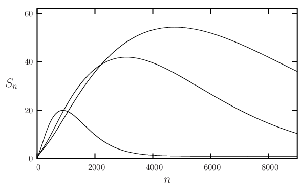
Let us now define a susceptibility by summing the above “response function” over the position of the constrained site. As there are on average sites at distance of the root, we have
| (104) |
We also define . Intuitively, is a measure of the “spine” of optimal rearrangements of size . By spine, we mean the subset of sites which belong to all of the optimal rearrangements for .
From Eq. (103), we get
| (105) |
The numerical solution of these equations is shown in the right panel of Fig. 18, for a few values of approaching . The behavior of these curves is strikingly similar to the one of the four point susceptibility close to the mode coupling transition in structural glasses Donati; Bennemann; FranzChi4A; FranzChi4B. Here plays the role of time in MCT, and that of the temperature. For a given value of , the spine size has a maximum which corresponds to rearrangements of total size . When both and diverge.
An analytical study of the asymptotic behavior, cf. App. C.5.1, confirms this remark. The main result is that scales as the typical size of large scale rearrangements, while , with an universal value . The same critical behavior was recently found for the for the four point susceptibility of the fully-connected -spin model, as well as in MCT BiroliBouchaud.
VII.3.2 Minimal barrier rearrangements
A geometric susceptibility can be similarly defined in terms of minimal barrier rearrangements. In this context, is the minimal barrier of a rearrangement for the variable which excludes , another variable at distance from . To simplify the analysis, we consider barriers obtained from the disjoint strategy. While exact barriers can only be computed through Yannakakis approach, we expect this simplification not to alter the critical behavior.
Following the same steps as in the previous Section, one is lead to define a function . This is the response of the minimum barrier distribution for site , to a perturbation applied on site . Using Arrhenius law, it is easy to establish the relationship between and physical observables. Assume that an external field has been applied to site at distance from . Let the expected (with respect to the graph ) local correlation function for spin , under the (equilibrium) modified Glauber dynamics. The response is given, in the low temperature limit, by
| (106) |
which generalizes to susceptibilities the relation (51) between barriers distributions and correlation functions. Unlike usual response functions (in which the external perturbation is infinitesimal), is the response to an infinite, but localized perturbing field. Since in any case as , this difference should be immaterial for the critical behavior.
Summing over the perturbation site , one can define a barrier susceptibility . Proceeding as in the previous Section, one can derive a set of coupled equations which determine :
| (107) | |||||
| (108) |
These are the counterpart of Eqs. (105) for size susceptibilities.
A numerical solution of these equations, cf. App. C.5.2, leads to the result shown in Fig. 19. As for the size susceptibility , the behavior of its barrier analog is very close to the one of the four point dynamical susceptibility in MCT. The barrier height plays the role of time, and in fact they are related through Arrhenius law in the low temperature limit, cf. Eq. (106). The maximum of corresponds to large scale barriers . Its height diverges at the dynamical transition , with the same universal value . The details of this analytic study can be found in App. C.5.2.
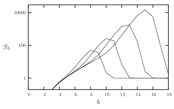
VIII Scaling analysis and numerical experiments
In the last Sections we focused on the zero temperature limit at . Here we shall discuss the implications of these results on the finite temperature behavior.
In order to simplify our discussion, we take a step back and focus on the global relaxation time . This is defined from the global correlation function through the condition 1616 16 As for local relaxaton times, cf. Sec. III.3 the precise value of is irrelevant, as long as it is smaller than the global Edwards Anderson parameter. Note also that the relaxation time introduced here should not be confused with other global time scales, such as the inverse spectral gap, or the mixing time. . Most of the arguments below can be easily transposed to local times.
In the low temperature, regime, Arrhenius law yields , where is the typical minimal barrier for large rearrangements. Substituting the critical behavior of , we get
| (109) |
This relation is valid if after . On the other hand, at any , the relaxation time does not diverge at , but at a somewhat higher value of corresponding to the dynamical line, cf. Fig. 1:
| (110) |
Equivalently, . In Sec. III.3, we derived a lower bound of this form implying .
Let now be some fixed small temperature, and consider the behavior of as is increased towards and above. We expect that (109) remains true as long as is not too close to . Near the divergence is rounded off, and eventually a crossover to the behavior (110) takes place. In other words, the dynamics crosses over from an “activated regime”, i.e. a regime for which Eq. (109) is accurate, to a “thermal” regime in which Eq. (110) holds.
At which values of does the crossover takes place? We will produce two distinct heuristic arguments that provide the same answer. The first one is very simple. The divergence (109) is rounded off only if is significantly different from . Equivalently, . On the other hand a cavity computation, cf. App. D, shows that, as ,
| (111) |
with a finite, -dependent constant. Therefore, the crossover regime corresponds to .
The second heuristic argument is more involved, but more instructive. A finite temperature configuration can be characterized through the locations of energy defects, i.e. frustrated interactions. In a low temperature equilibrium configuration, these defects are very sparse, and their density is about (as long as ). Consider now a spin , and the associated minimal barrier rearrangement of size and barrier . Glauber dynamics will make use of energy defects in order to accelerate the relaxation of , with respect to the purely activated behavior . A rough intuition of this phenomenon is obtained by assuming that interactions containing an energy defect can be removed from the system. A first remark is that, as long as , no energy defect is encountered along the activated path (also allowing for slightly sub-optimal rearrangements). Arrhenius behavior is therefore not modified. Focusing on large rearrangements, this implies that Eq. (109) remains correct as long as (i.e. ).
This simple minded argument can be refined. We expect an energy defect to be as effective in reducing the effective barrier seen by spin , as a pinning field is in augmenting it. In other words, the density of such defects must be compared to the size of the large rearragements spine (i.e. to the peak of the geometric susceptibility), rather than to their overall size. Using the results of Sec. VII.3.2, we conclude once again that the crossover regime corresponds to .
What is the behavior of in the crossover regime? Inspired by the anomalous dynamical scaling for diluted ferromagnets at the percolation transition Henley; Rammal we conjecture the scaling form1717 17 The differences with respect to the form in Ref. NostroLettera are due to a different normalization of the temperature.
| (112) |
In order to match Eqs. (109) and (110), the scaling function must have the following asymptotic behaviors
| (113) | |||||
| (114) |
where .


We carried out extensive numerical simulations in order to check this scaling hypothesis, along the lines exposed in Sec. VI.6. In Fig. 20, left frame, we reproduce the resulting global correlation time for several values of as functions of . In Fig. 20, right frame, we check Eq. (112) by plotting , in rescaled units, for several values of and . Despite the variation of the relaxation time over several orders of magnitude, an acceptable agreement is found. Remarkably, Eq. (112) predicts a super-Arrhenius divergence at this value of : . The prediction is well verified by numerical data, cf. Fig. 21, thus supporting the hypothesis made in computing , cf. Sec. VI.

While the numerical results do not prove unambiguously Eq. (112), they support it as a valid working hypothesis. As in the case of diluted ferromagnets, Eq. (112) is consistent with temperature being a relevant perturbation (in renormalization group sense) at the critical point . This in turns suggests that the line is ruled by a different universality class with respect to this point.
IX Conclusion
In Section II.1 we stressed that the critical dynamics of Bethe lattice models was understood only in the fully connected limit. In the previous pages we derived several results concerning the opposite limit , . We can now leverage on the knowledge concerning these two extremal points, in order to propose a complete scenario for the whole dynamical line .
We found two universality classes1818 18 We use the term “universality” despite its content is not as clear in the present context as it is for ordinary critical phenomena. which correspond to distinct divergences of the slow time scale:
- •
- •
On the other hand, several important elements are common to the two universality classes. Among the others, the linear size of cooperative regions scales as , and the peak of the dynamical susceptibility as , with and (here for the first class, and for the second) BiroliBouchaud.
In Sec. VIII we argued that temperature is a relevant perturbation at the point. It is therefore natural to guess that the whole , is controlled by the ordinary MCT class. Namely, there exist a continuous function , such that the slow time scales behaves as in Eqs. (36), (37). The crossover away from the point is described by Eq. (112). Finally the cooperativity exponents and remain constant on the whole line, as well as in the crossover regime.
At any finite temperature, usual MCT behavior eventually overcomes aMCT when the system is close enough to the dynamical line. On the other hand, activation can be important in a large pre-asymptotic regime, depending on the way the dynamical line is approached. Such a regime can be of experimental interest.
In the model studied in this paper, the crossover is controlled by the scaling variable . This can be interpreted as the ratio between two diverging sizes at the point: the spine of large scale rearrangements, which scales as , and the inverse density of energy defects scaling as . In terms of observable quantities, we could have written , where is the system specific heat, and is the peak value of the dynamical four point susceptibility. In more general (non-mean field) systems, the same role is likely to be played by a ratio of the form . Here is a thermal correlation length, and is a dynamical correlation length extracted from four point dynamical correlations. A similar scaling variable describes the crossover in diluted ferromagnets at the percolation point Stinchcombe.
The methods developed in this paper can certainly be applied in a more general context. In particular, rearrangements can be defined for kinetically constrained models (Kob-Andersen, Frederickson-Andersen for instance) on Bethe lattices, and studied along the same lines NostroKCM. Interestingly, a recent numerical study EPL_MauroCristinaGiulio has investigated the relaxation time divergence in these models and indicates a behavior of the type ( being the particle density).
As we mentioned in the Introduction, the problem studied here is known in computer science as XORSAT, and is a simple example in the wider family of random Constraint Satisfaction Problems CSP. The dynamical glass transition, essentially studied in this context at zero temperature as a “clustering transition” of the groundstates, is a feature shared by other examples of this family, Satisfiability and Coloring in particular SAT; Coloring. It would be of great interest to extend the refined decription of the changes in the landscape properties at the clustering transition we obtained in the XORSAT problem to these other models.
Acknowledgments
This work has been partially supported by the integrated project EVERGROW (n. 1935 in the complex systems initiative of the Future and Emerging Technologies directorate of the IST Priority, EU Sixth Framework), and the Research Training Network STIPCO (HPRN-CT-2002-00319).
Appendix A Properties of the equilibrium distribution
We prove here the statements and made in Section II.1. In order to prove , notice that the partition function admits the usual high temperature expansion
| (115) |
where the (finite) sum over runs over all the hyperloops in . denotes the size of the hyperloop and the product of the signs of the interactions in it. If no hyperloop is present, only the first term survives.
Consider now . Let be the distribution of the sign of the quenched couplings, i.e. the uniform distribution over , and the Boltzmann distribution for the configuration , given the couplings . Sampling from and then from the conditional distribution is equivalent to sampling from the joint distribution
| (116) |
Using the form of the Boltzmann distribution, we have
| (117) |
This is in turn equivalent to sampling form the marginal distribution and then from the conditional distribution . We are left with the task of determining these distributions. Using the definition of marginal distribution, and the fact above, we get
| (118) |
i.e. the marginal distribution of is uniform. We can now apply the definition of Bayes theorem to get
| (119) |
which proves our claim.
Appendix B Correlations
This Appendix contains the technical details of the calculation of equilibrium correlation functions presented in Section III.
B.1 -point correlation functions: zero-temperature potential
We start by computing the annealed potential (10). By taking expectation with respect to the graph , and the constrained spins (but not on their number), it is elementary to obtain
| (120) |
Here the sum runs over . Let us define the annealed potential at size as . By a standard saddle point calculation, we get
| (121) | |||||
| (122) |
Here is the function maximized in Eq. (10) and is the point realizing the maximum. As , we have .
As claimed in Sec. III, given , for any with high probability. Let us stress that this statement is stronger than saying that, given , with high probability. On the other hand, it is required in order to estimate the derivatives of . It can be proved by distinguishing two regimes (here ): and . In the first regime, the term in Eq. (120) can be replaced by . The relative error is of order , yielding . Since is a power of by definition, the probability that is at most (recall that is an integer). The desired result is obtained by taking expectation with respect to .
In the second regime, we apply Markov inequality to the random variable (here we condition on a typical value of ):
| (123) |
The term can be safely estimated by (deviations of from being exponentially rare). The right hand side of the above expression is therefore (neglecting small error terms) . For any finite (as ) , . If (but ) . Therefore the probability that is exponentially small.

In Fig. 22 we plot the function for , and a few values of . For , has a global maximum at with in its neighborhood. This implies the expansion (11). The same is not true for because a second local maximum at overcomes the first.
The value of in the thermodynamic limit can be computed through the cavity method. Alternatively, one can use a leaf-removal argument in the spirit1919 19 We also refer to Luby; Maxwell for an analysis of this algorithm on graph ensembles with general degree distributions. The results of Maxwell include Eq. (124). of Refs. XOR_1; XOR_2. We get
| (124) |
For and , the is realized at . A straigthforward calculation yields
| (125) |
in agrement with the rigorous bounds (12). Higher derivatives can be computed as well and are finite for any . In particular, the third derivative is easily seen to be related to the three points susceptibility , in analogy with Eq. (9). Under the assumption that the limits and can be interchanged, this implies the finiteness of for , and .
B.2 -point correlation functions: cavity argument
The argument of the previous Section could be generalized to finite temperature using the Franz-Parisi quenched potential FranzPotential. A more direct calculation consists in computing the correlation functions using the cavity method.

In order to simplify the exposition, consider the three-points function for . Generalizing to the computation of connected correlation functions as well as to other values of and should be straightforward. As a further simplification, consider the example in Fig. 23 and , , . The one-step replica symmetry breaking (1RSB) cavity expression for reads
| (126) |
Here is Parisi 1RSB parameter,
| (127) | |||||
| (128) | |||||
| (129) |
and . Finally is the 1RSB spin glass order parameter, i.e. a distribution over the space of symmetric distributions on : .
If (which is the case for ), these expressions simplify remarkably. One can in fact integrate explicitly over the . Since is symmetric, does not depend on . The espression in curly brackets in Eq. (126) is therefore given by
| (130) |
An analogous expression holds for . Taking the ratio and integrating over , we get the final result
| (131) |
Notice that the cavity fields on the right hand side are set to . In particular, for the case at hand . More generally is different from only if are connected by an interaction . In this case we get . Proceding analogously, one can show that and therefore . Summing over all the triples we find that, in the thermodynamic limit,
| (132) |
for any . Proceeding analogously, one can compute higher order susceptibilities for any finite .
B.3 Point-to-set correlation functions at finite
In this Appendix we explain how to compute the point-to-set correlation length and show that it diverges at . Recall that the dynamical transition is usually defined using the following equations (one-step replica symmetry breaking with Parisi parameter )
| (133) | |||||
| (134) |
where . The fields distributions and are required to be symmetric. The indices and refer to nodes in the factor graph. When a random factor graph is considered, and become i.i.d. with common distributions (respectively) and , and becomes a Poisson random variable with mean . The above equations acquire a distributional meaning. is defined as the largest temperature such that a non-trivial solution exists for these distributional equations with .
Using the symmetry of , it is easy to show that for . We can therefore average over and . If we call, respectively and the average distributions, we get
| (135) | |||||
| (136) |
Consider now the calculation of the point-to-set correlation length . First notice that, within the high temperature phase the cavity fields vanish identically. This means that an equilibrium configuration within a neighborhood of a site can be constructed as follows. First fix uniformly at random. Then for any of the interaction terms involving , let us say , generate the other spins from the distribution
| (137) |
Then repeat the same operation with those neigbors of spins (as well as of the other neighbors of ), which have not yet been fixed. Repeat recursively until all the spins within a distance from are determined. This procedure is well defined, because the factor graph is a tree within any fixed distance from .
Notice that, in order to generate the values of the spins adjacent to , we did not need to know the graph structure at any distance from larger than . As a consequence, a random graph and a thermalized configuration for that graph can be generated jointly as follows (in the thermodynamic limit). First generate the degree of site from a Poisson distribution with parameter . Then generate the values of the spins which interact with , according with the rule given above. Repeat the same operation for the neighbors of , and continue recursively for any fixed distance .
This gives a procedure for constructing the reference configuration in our definition of , cf. Eq. (24). The recursive nature of this procedure allows for a recursive calculation of . Condition now on the event that and constrain a copy of the system to have spin at site , for any whose distance from is at least . Let be the effective field acting on site under this boundary conditions. This is of course a random quantity, because the reference configuration as well as the underlying graph are random. Denote by its distribution, and by its distribution under the condition that the degree of is exactly . Then, it is easy to derive the recursions (here we assume, for the sake of simplicity, , and use the shorthand )
| (138) | |||||
| (139) |
which hold for any , together with the boundary condition
| (140) |
These recursions can be easily approximated numerically using the population dynamics algorithm of MezardParisiBethe. Notice that, by construction, and and therefore a unique population need to be tracked. Furthermore, the recursion preserves the following property
| (141) |
The point-to-set length scale can be estimated by computing the quantity (here denotes expectation with respect to the sample realization)
| (142) |
The data shown in Fig. 4 have been obtained using this approach.
At high enough temperature, the iteration (138), (139) converges to the trivial fixed point . As the temperature is lowered, the convergence becomes slower and slower, and the plot of develops a plateau as a function of . Eventually, the iteration converges to a non-trivial fixed point of Eqs. (138), (139), let us denote it by , . Exploiting the property (141) we can rewrite the fixed point distributions as
| (143) |
with and two symmetric distributions. Rewriting the fixed point condition, cf. Eq. (138), (139) in terms of and , we recover the 1RSB equations (135), (136). We thus proved that the existence of a non trivial fixed point for the 1RSB equations is equivalent to the existence of a non trivial fixed point for the recursion (138), (139). Under the assumption that, as soon as such a fixed point appears converges to it2020 20 A proof of this assumption in a similar problem, due to J. Martin and E. Mossel, is reported in Ref. Reconstr., we thus proved that for .
Appendix C Asymptotia
In this series of Appendices we shall work out the rearrangement critical behavior, i.e. both at and as . Throughout these Appendices will denote the distance to the critical point.
Before embarking in the calculations, it is interesting to draw some parallels with the analytical treatment of the schematic MCT model, and to collect technical properties we shall use in the following.
The time correlation function of the schematic MCT (or of a fully-connected spherical spin-glass model at high temperature) obeys an equation of the form
| (144) |
where the memory kernel is a polynomial of the correlation function itself, . These two equations share some features with the ones governing the distribution of minimal size rearrangements, cf. Eqs. (43), (44): the first one is a convolution on (resp. on ), the second a polynomial relation between and (resp. between and ). In both situations, one of the equations is simple in the “direct space” of or , the other being simpler in Laplace transform (or generating function, see below).
As for MCT, the study of (and similar quantities) in the critical regime, can be carried out in three steps. First, one considers its decay exactly at the critical point, with (or ) fixed. In a second step, one identifies an “intermediate regime” which describes around its plateau value. Matching these two regimes yields the scale of in the intermediate regime. The “final regime” describing the decay of from its plateau to zero can also be described by a scaling function. Again, the corresponding scale of is derived through a matching argument.
Given a function defined for , the corresponding Laplace transform will be denoted as
| (145) |
The equivalent of Laplace transform for discrete variables is given by generating functions (g.f.). We refer to Wilf; Odlyzko; Flaj_book for an extensive introduction to generating functions and asymptotic combinatorics methods, and recall here a few basic definitions. Given a sequence defined for , the associated g.f. is the formal power series
| (146) |
As for Laplace transform, convolutions of discrete sequences translates into products of the corresponding generating functions. We shall sometimes introduce (right) partial sums of a sequence, denoted with the same upper-case letter:
| (147) |
The corresponding g.f. and are then related by
| (148) |
The asymptotic behavior of a function shows up in the singularities of its Laplace transform. For instance, if when , then
| (149) |
where denotes a function having milder singularities than at . A formally identical formula holds when when (in this case one has to look at ).
Similar relations holds for generating functions. If for large , then the associated generating function behaves as follows near :
| (150) |
C.1 Minimal size rearrangements
Throughout this Section, we shall denote by (respectively ) the generating function of the distribution (resp. ) of rearrangements minimal sizes. With this notation, Eq. (43) can be written as
| (151) |
C.1.1 Order parameter
Let us first determine the order parameter of the transition, that is to say the fraction of variables with diverging minimal rearrangement sizes. This is defined as . Similarly, let . From Eq. (44) one obtains , whereas Eq. (151) evaluated at leads to
| (152) |
This has a non vanishing solution only for , where is the critical point defined in Eq. (19). The critical point and the value of the order parameter at this point can be determined by the two equations
| (153) | |||||
| (154) |
The last of these equations expresses the fact that the two functions of on the left and right hand sides of Eq. (152) become tangent at when .
C.1.2 Critical decay
We shall first place ourselves right at the transition, , and study the decay of towards its asympotic value . Define and . The generating functions are given by
| (155) |
and a similar expression for . In terms of these quantities, Eq. (44) becomes .
Guided by the numerical solution of Eqs. (43), (44) we look for an asymptotic behavior of the form as . Here is a positive exponent and a constant. Equivalently . Expanding the relation between and , we obtain
| (156) |
Our aim is now to determine the decay exponent , by matching the singularities around in the equation on the generating functions.
Using Eq. (150), we obtain as . Assuming , we apply the same formula to :
| (157) | |||||
| (158) |
We can now plug these formulae in Eq. (151), and match the two sides order by order as . The terms of order are equal thanks to the equation (153) on the order parameter. The terms proportional to (of order ) match because of Eq. (154). Next, on the r.h.s. of Eq. (151) two terms of order appear (while none is present on the l.h.s.): one is proportional to , and the other to . Requiring them to cancel yields the relation (45) which fixes the exponent .
The l.h.s. of Eq. (45) is shown in Fig. 6. As long as , the equation has a unique solution in . The exponent is given by this solution, thus verifying the hypothesis . It order to show that for any , we use Eq. (154) to simplify the expression for :
| (159) |
Using the inequality in Eq. (153), we obtain . Thanks to (154) we get , which in turns implies the thesis.
C.1.3 Intermediate regime
We shall now study the behaviour of the probability law of the minimal rearrangements sizes slightly below the critical connectivity, i.e. as .
Inspired by the distribution of zero-temperature point-to-set correlation lengths, studied in Sec. III.2, we guess that an intermediate scaling regime emerges when . Using the results of the previous Section, we expect this to happen on a scale . For the time being, we only assume that diverges at more rapidly than .
In order to blow up around its plateau, we define, for any
| (160) |
and similarly . Using Eq. (44), we get
| (161) |
In order to describe the plateau regime, we must properly rescale the generating functions as :
| (162) | |||||
| (163) |
In order to estimate the remainders, we assumed that is smooth for and has a singularity at which is milder than .
We can plug these formulae for and , into Eq. (151) and compare the two sides order by order in . The terms of order and match because of Eqs. (153) and (154). On the contrary the order determines the function via
| (164) |
where , and has been defined above. Inverse Laplace transforming the equation yields to
| (165) |
From this equation one can determine the asymptotics of , which turn out to be:
| (166) |
where is the exponent already found in the previous Section, and is the positive solution of Eq. (47).
This allows us to fix the scale . Consider indeed large (but independent of ) values of , and the limit . From the study of the previous Section at , we know that . From the behavior of we have . Consistency in the limit implies thus , confirming the qualitative argument given in the beginning of this Section.

In Fig. 24 we use the numerically determined distribution in order to check the scaling form used in this Section.
C.1.4 Final regime
At what size scale does exit the plateau regime and decreases by a finite amount below ? Using the intermediate regime scaling, we have . From the behaviour of at large , we get , where
| (167) |
In order to describe this regime, we define the scaling limits
| (168) |
and analogous ones for and (with scaling functions and ). As usual, the scaling limits of generating functions are related to Laplace transforms: , . Equations (44) and (151) imply
| (169) |
This set of equations determines , the scaling function of the decay of between and (this function was denoted as in Sec. V.3). In particular they imply . This behavior can be matched with the intermediate regime, cf. previous Section, and can be used to confirm that .

C.1.5 Extreme decay
What is the probability of an “anomalous” minimal size rearrangement, i.e. a site such that is much larger than for most of the other sites? This question can be answered by studying the asymptotics of the sizes distribution .
It is convenient to consider first a slightly modified model, in which the maximum allowed variable degree is a finite number as . We refer to Bollobas for graph ensembles of this type. It is easy to generalize our treatment to such graphs: Eq. (44) remains unchanged, while Eq. (151) is modified to
| (170) |
Here is the probability that an edge chosen uniformly at random in the factor graph is adjacent to a variable node of degree .
A numerical investigation of Eqs. (44) and (170) suggests the Ansatz
| (171) |
with . Equation (44) implies . The corresponding generating functions can be estimated through the saddle point method. We get
| (172) |
as . The analogous expression for is obtained replacing by in the last formula. Inserting into Eq. (170) and matching the leading term as determines the exponent
| (173) |
In other words, the probability of very large rearrangements decreases faster than exponentially. In a given graph of size , the largest minimal size rearrangement can be estimated by setting , which implies
| (174) |
Let us now reconsider the original model, with unbounded degree. The expression (173) yields . A more careful study shows that
| (175) |
where is a function diverging as , but more slowly than any iterated logarithm2121 21 More precisely, it is a solution of the Abel equation Kucma . (i.e., for instance, than ), and is a positive constant.
C.2 Minimal barrier rearrangements
We present in this Appendix the resolution of Eqs. (60) on the distribution of minimal barriers. We shall first discuss a more general class of distributional equations. The representation developed in this context is then used to solve numerically Eqs. (60). Finally, we analyze the critical behavior of its solution.
C.2.1 Transformation of the permutation functionals
Equations (60) involve functionals of the probability distribution which can be generalized to the following problem. Consider integers (fixed) , that without loss of generality we assume to be ordered, , and define a function of other integers by
| (176) |
where the minimum is over the permutations of . Assume the ’s to be i.i.d. random variables with distribution . What is the distribution of ? Its cumulative distribution is
| (177) |
which is a functional of the law .
A first simplification is that the minimum in the definition of is achieved for a permutation which orders the ’s by their value (and any such permutation is equivalent). In other words with . Now one has
| (178) |
It is useful to represent the ’s in a slightly different form. Let us call the number of distinct elements in the set , and their values. The degeneracies of the are encoded in the coefficients defined for as the number of strictly smaller than . By definition one has . As an example, if for , , one obtains , and . These definitions can be used to remove the redundant constraints of Eq. (178): if for instance , as the ’s are decreasing. These eliminations lead to
| (179) |
We now come back to the original variables and define , for , as the number of ’s strictly smaller than . This imply that
| (180) |
We thus have . We can now insert Eq. (179) in the definition (177) and trade the sum on the against a sum on the respecting the above derived constraints.
| (181) |
The combinatorial factor arises from the change of variables from the ’s to the ’s, and the constrained sum is over
| (182) |
In the following, we shall repeatedly use the representation of provided by (181), (182).
Before leaving this general preliminary, let us note that if the ’s are bounded from below by (i.e. for ), is bounded from below by , hence for .
C.2.2 Application to the -spin model and numerical resolution
The equations (60), determining the barrier distribution of the -spin model (1), can be rewritten as
| (183) |
where is of the general form studied in the previous pages, with the ’s drawn with the law , and the ’s given by . Here we set by convention .
Following the notations of the previous Section, one has for a given value of : , , and for . As the law is supported on the positive integers, for . This allows to rewrite the equation (183) under the form:
| (184) | |||||
| (185) |
with the constraints on the sum in :
| (186) |
These equations allow to determine the distribution of messages , defined in Sec. VI.3 (anchored barriers). The distribution of actual barriers to flip a spin in the system can be expressed in a similar way,
| (187) | |||||
| (188) |
with the constraints on the sum in :
| (189) |
By convention the products from to which appear in are equal to 1.
Unlike for the minimal size distribution, Eqs. (183) do not provide immediately an algorithm for computing by recursion over . The reason is that the anchored barrier of a rooted tree is at least as large, but not necessarily larger, than the anchored barriers of its sub-trees. Consider now the process of merging sub-trees (this corresponds to iterating (183) once). If sub-trees barrier distribution are known only up to barrier height , the barrier distribution of the new, larger tree is necessarily undetermined at height .
We can propose two ways to solve this difficulty. The first one is to derive a well-behaved recursion on . Assume that and (resp. and ) are known upto height (resp. ). The only unkwnown of the right hand side of Eq. (184) is , which appears linearly because of the conditions in the sum (185). We can thus write
| (190) |
where the coefficients and are computable from using Eq. (185). Using , and , one ends up with
| (191) |
One can solve this equation for (recall that is assumed to be known at this stage) and therefore determine , and . This allows to continue the recurrence at the next barrier height.
The second method is iterative: make an initial guess for the law , compute the law , cf. Eq. (183), and inject it in (184) to recompute . Any fixed point of this procedure corresponds to a solution of Eqs. (183). Since the solution is unique, whenever the procedure converges, it provides a good numerical approximation of this solution. It can be argued2222 22 A complete proof is beyond the scope of this Appendix. The basic idea is that the function obtained after iterations, is the minimal barrier distribution for a subgraph of radius around a random node . Convergence follows from the remark that this barriers become larger (and therefore worsen, in a sense that can be made precise) as increases. that the iterative procedure indeed converges for any , if the initial condition is used.
C.2.3 Asymptotics
In this Appendix we work out the asymptotic behavior of minimal barrier distributions, cf. Sec. VI.5. Motivated by the results on minimal size rearrangements, cf. Sec. C.1, we look for a plateau at , . We thus define
| (192) |
With this definition one can set up an expansion of the functionals in powers of . We shall need in the following this expansion upto terms of order . Four types of terms appear at this order in Eq. (185) :
-
, which gives a term of order 1.
-
, , with , of order .
-
, , with , of order .
-
, , , with , of order .
Summing this terms and expanding the result upto order , we obtain:
| (193) |
Inserting this expansion in Eq. (184), assuming (we are interested in the large behavior) leads to
| (194) |
Since we are interested in the large behavior, we can extend the sum on upto infinity with a negligible error2323 23 More precisely, we shall eventually focus on , and retain terms in this equation up to . On the other hand, extending the sums up to produces errors of order (to the leading exponential order).. Moreover we can expand the first equation in (183) to express in terms of . Ordering the different powers of , we get
| (195) |
We now consider the critical limit infinitesimal. The two terms in brackets vanishes at , because of Eqs. (153) and (154). Expanding also in powers of , we obtain
| (196) |
where and are as defined in App. C.1, cf., for instance, Eq. (164).
Notice that Eq. (196) is simpler than the analogous equation for minimal size rearrangements, i.e. Eq. (164). In particular, it is not necessary to introduce generating functions or Laplace transforms: Eq. (196) is local in the “direct space” of barriers.
Let us consider first the large behavior at the critical point . The left hand side of (196) vanishes (as well as all corrections proportional to ), and one can look for a solution such that as . Injecting this Ansatz in Eq. (196) and requiring the terms of order to cancel yields the condition , which fixes , as announced in Eq. (62).
In order for Eq. (196) to have a non-trivial limit within the plateau regime, we must have in this regime. We therefore assume the existence of a diverging scale , and define . Substituting in Eq. (196) and taking the limit, we get
| (197) |
It is easy to work out the asymptotic behavior of the solution of this equation. We get as , and as , where is given by Eq. (64) and are two positive constants.
The scale is fixed by matching the behaviour of at for with the one of when . Consider a large (but independent of ) value of , and the limit :
| (198) |
The dependence on cancels only if . In Fig. 26, left frame, we plot the outcome of a numerical resolution of the equations (183) along the lines exposed in the previous Section. The data are rescaled in such a way to exhibit the plateau scaling. More precisely, we plot
| (199) |
for several values of , as a function of . The good collapse of the curves confirm the analysis just presented.
Notice that the quantity (199) is not expected to converge to a unique curve as a function of , even if is chosen optimally (here we just derived its asymptotic behavior). In other words, is not a scaling function in the usual sense. The reason is that Eq. (197) has more than one solution, and two such solutions and cannot be superimposed through a shift of the axis (this is related to the fact that is discrete). On the other hand, a shift can be found such that . Therefore the function (199) will converge, as a function of , within a distance around any solution of Eq. (197). This is enough for the analysis presented in this pages to be valid.
Finally, the scale for the decrease of from to , can be defined as the smallest such that with any fixed number smaller than . It can be estimated by requiring to be of order 1, or, equivalently, to be of order . This implies , i.e. , hence
| (200) |
as announced in Eq. (65).
Figure 26, right frame, shows (obtained from the numerical resolution of Eqs. (183)), as a function of . The curves for different values of collapse between 0 and , thus confirming our analysis.
Contrary to the minimal size case, one cannot define a scaling function for the last decay from the plateau value to 0. Indeed, this happens on an interval of which remains of order 1 when . This means that a finite fraction of the barriers is not just of order , but within a finite additive constant from .
This asymptotic study has been performed on the distributions and of the messages on the links of the factor graph (anchored barriers). However, actual barriers to spin flips differ at most by one from anchored barriers. The discussion presented so far is thus also valid for the actual barrier distribution .


C.3 Average size of minimal barrier rearrangement
Let us explain how to derive the results presented in Sec. VII.1 on the average size of minimal barrier rearrangements. To this aim one has to solve Eqs. (81) and (82). The first of these equations involves a constrained sum on anchored barriers , whose disjoint combination leads to a prescribed barrier . This is similar to Eq. (60) (first equation) that was solved in App. C.2. Unlike in Eq. (60), one of the barriers is not drawn from the distribution , but is the argument of the unknown sequence . Let us define an integrated version of this sequence (as well as of the related ),
| (201) |
Notice that, at odds with our usual conventions we integrated to the left. Equation (81) can thus be rewritten as
| (202) |
The sum in can be transformed following the strategy exposed in App. C.2, treating the distinguished indice separately from the others. A similar reasoning leads indeed to
| (203) |
where the parameters of the sum obey the following constraints:
| (204) |
We have encoded the value of the special indice in the sequence of the , with . The form (203) is suitable for numerical resolution of Eqs. (81), (82), following one of the two strategies (recursion or functional iteration) explained in Sec. C.2.2.
Let us now study the asymptotic regime . Following the notations of App. C.2, we can expand Eq. (203) in powers of :
| (205) |
Inserting this expansion in Eq. (202), and extending the sum on to infinity (as in Sec. C.2.3, this produces a negligible error) leads to
| (206) |
Expanding also Eq. (82) to the same order yields
| (207) |
Next we take finite differences of Eq. (206) and trade for , thanks to (207), and for , thanks to Eq. (44). We finally get
| (208) |
As usual, we consider three distinct asymptotic regimes. Let us begin by assuming and large. The l.h.s. of Eq. (208) vanishes because of Eq. (154). Moreover, we know from App. C.2.3 that . Numerical computations suggest the Ansatz , with . Under this Ansatz terms of order and can be safely neglected in Eq. (208). Requiring the r.h.s. to vanish to the leading order , yields the condition
| (209) |
It is not hard to show that the above equation admits a unique solution larger than , thus completely determining the exponent . For instance when one obtains .
Consider now the intermediate regime, , with , where and is finite. We found in this regime a scaling function , such that . Let us introduce now a similar scaling function for the ’s, , with a still unknown exponent that we assume to be larger than . With this assumption, the dominant terms in Eq. (208) are of order . Imposing Eq. (208) to hold at this order, we obtain the following equation for the scaling function :
| (210) |
We found in App. C.2.3 that (resp. ) in the (resp. ) limit. Using these results, one can derive the asymptotic behaviour of in these two limits. When , we have , where is the exponent previously determined. When , , where is the unique positive solution of
| (211) |
For instance, we obtain for .
The exponent is obtained by matching the limit of the solution, and the limit of the intermediate regime:
| (212) |
For the dependence on to cancel, we have to take . Note that the assumption is a posteriori confirmed, as .
This analysis of the intermediate regime is confirmed by Fig. 27. Here we plot , versus , with computed numerically for several values of , and determined analytically as explained above.

Finally, we look for the asymptotic behavior of when the typical height of large minimal barriers (recall that ). From the behaviour of when , we get
| (213) |
As is of order 1 in this regime, the exponent is indeed the one which controls the divergence of , the average size of large scale minimal barrier rearrangements.
C.4 Average distance in minimal sizes rearrangements
We study in this Appendix the asymptotic behaviour of the solution of Eqs. (93). This allows to compute the average radius of minimal size rearrangements. Let us denote and the g.f.’s associated repectively to and . The first of equations (93) can be rewritten as
| (214) |
where is the g.f. of the ’s.
Consider first the solution at . From the results of Sec. C.1 we have the following asymptotic behaviors as ():
| (215) | |||||
| (216) | |||||
| (217) |
Motivated by the numerical solution of Eqs. (93), we assume that, when , admits a finite limit as . This implies as . Using the second of equations (93), together with the formulae (216), (217), we get
| (218) |
Plugging this Ansatz in Eq. (214) along with the expansion (215), one realizes that terms of the type (with an -independent constant) cancel because of Eq. (154). The leading surviving terms are of order . Imposing them to vanish, we get
| (219) |
Let us now turn to the intermediate regime, on the scale , and define the scaling variable . We found in Sec. C.1.3 that
| (220) | |||||
| (221) | |||||
| (222) |
where is the scaling function of around the plateau, introduced in Eq. (160).
Let us make the following Ansatz on this scale:
| (223) |
In this regime, the second of equations (93) reads
| (224) |
Next we insert this formula in Eq. (214) and expand in . Leading order terms are of the form (of order ), and cancel as usual. The scaling function is is determined by the vanishing of terms, which leads to
| (225) |
Studying the limit of this equation, one can check that reaches for small the value determined above, fulfilling the consistency condition between the end of the finite regime and the beginning of the “intermediate” one. Consider now the limit , and assume , with a yet unknown positive exponent. Recalling that as , the above equation yields:
| (226) |
It follows from the convexity of for that this equation has a unique positive solution, which, because of Eq. (47), is .
Finally, let us turn to the large rearrangements regime, , with . We define scaling functions on this last scale by
| (227) |
We defined in App. C.1.4 the scaling function for the minimal size distribution in this regime. From this definition, we have
| (228) | |||||
| (229) | |||||
| (230) |
These last two formulae allow to relate and , using the second of equations (93). Assuming (which is consistent with the outcome of numerical computations), we get
| (231) |
Injecting this expression in Eq. (214), we finally obtain an equation determining the scaling function ,
| (232) |
Using Eq. (169), it is not hard to show that is, for any , a solution of this equation. This solution yields for , consistently with the above study of the intermediate regime.
A matching argument allows to fix the exponent . Consider indeed , with but independent of . From the limit of the intermediate regime we have . Consider instead the limit of the final regime, we get
| (233) |
Matching the two asymptotics, we obtain the universal exponent .
Let us finally compute the quantity , i.e. the average radius of a rearrangement of size . Using the above solution we find, on the scale of large minimal size rearrangements :
| (234) |
C.5 Geometrical susceptibility
In this Appendix we work out the critical behavior of the geometrical susceptibility defined in Sec. VII.3.
C.5.1 Minimal size rearrangements
The susceptibility for minimal size rearrangements is determined by solving Eqs. (105). It is helpful to rewrite the first of these equations as
| (235) |
As usual, we start by considering the large behavior at . Numerical computations suggest the Ansatz , with an exponent to be determined. From the second of Eqs. (105), and recalling that , we get
| (236) |
This implies in particular . This expression can be substituted in Eq. (235). The leading terms are of the type (and of order ) and cancel because of Eq. (154). We get an equation of the form
| (237) |
where is -independent and given by
| (238) |
and is the constant already introduced in Sec. V.3. Notice that Eq. (237) cannot be satisfied for (in this case, it would imply ), nor for (it can be shown2424 24 Consider the expression in curly brackets in Eq. (238) (the prefactor is positive). Proving that it is negative is equivalent to proving that , where . This in turns follows from the fact that is strictly convex for . that for ). Therefore we have necessarily , and Eq. (237) determines the prefactor .


Next we consider the intermediate scale . Since at , we expect for and . We assume the scaling behaviour
| (239) |
with an analogous Ansatz for (with scaling function ), and an exponent yet to be determined. Equations (105) yield (cf. also the form (235))
| (240) | |||||
| (241) |
Eliminating , we obtain an equation determining the scaling function . For we get:
| (242) |
Other values of can be excluded via an analysis of the resulting equations: we shall stick to hereafter. The asymptotic behavior of the solution of Eq. (242) can be determined by recalling that as , and as . We get for and for . The choice is confirmed by matching the behavior with the analysis of the finite regime, explained above.
In Fig. 28, left frame, we plot versus , with determined via a numerical solution of Eqs. (105). The good collapse confirms the validity of the above analysis.
Let us finally consider the scale of large rearrangements , and assume in this regime
| (243) |
with an analogous Ansatz for , and a new critical exponent. Injecting this form in Eqs. (105), and recalling that on the same scale, we get:
| (244) | |||||
| (245) |
Studying these equations in the limit allows to determine the asymptotic behaviour as . This allows to determine the exponent through a matching procedure. If we let , with large but –independent, from our study, respectively, of the intermediate and final regimes, we get
| (246) |
This in turn implies .
C.5.2 Minimal barrier rearrangements
This part of the Appendix is devoted to the resolution of Eqs. (107,108) for the geometric susceptibility of minimal barrier rearrangements. Using the fact that , Eq. (107) can be rewritten as
| (247) |
The quantity is very similar to defined in Eq. (202), with the sequence replacing . In particular admits a representation of the form (203), where is replaced by . The numerical computation of proceeds along the lines exposed in Sec. C.3.
The expansion of Eqs. (107), (108) in powers of is also analogous to the one of Sec. C.3. We get
| (248) | |||||
| (249) |
Next we eliminate from the above equations and assume the asymptotic behavior , with to be determined. Recalling that , we get
| (250) |
where
| (251) |
and is defined in Sec. V.3. Using an argument similar to the one in the previous Section, one can show that Eq. (250) implies .


Let us consider now the intermediate regime , where and . Inserting the Ansatz in Eqs. (248), (249), dominant terms (of order ) cancel. For next-to-leading terms to cancel, one has to choose . The scaling function is then found to obey
| (252) |
The asymptotic behaviour of can be deduced from this equation, using the results on , cf. Sec. C.2.3. One finds as (thus matching the behavior in the first regime) and as .
In Fig. 29, left frame, we compare the postulated scaling in the intermediate regime with a numerical solution of Eqs. (107), (108).
Finally, on the large rearrangement scale , we expect . The exponent can be determined by matching this behavior with the large asymptotics in the intermediate scale:
| (253) |
We thus have as claimed in Sec. VII.3.2.
Appendix D Low temperature behavior of the dynamical line
In Sec. VIII, we claimed that the dynamical transition line behaves as described in Eq. (111) in the low temperature limit. A proof of this statement requires a particularly involved asymptotic calculation, and goes beyond the scope of this paper. On the other hand, a simple argument can be constructed as follows.
Consider and expand the solution of the 1RSB equations (133), (134) as , with and fixed. At , the order parameters , concentrate over local field distributions , supported on integer fields . More precisely, with probability (corresponding to hyperedges in the backbone), and with probability (hyperedges outside the backbone). Analogous expressions hold for .
A small non-zero temperature has two effects on . First of all, any local field distribution in the support of aquires a peak for . Second, the peaks on integer fields acquire a small width. In general, this width is of order and the last effect dominates. For XORSAT, the width is of order and can be neglected to first order (this can be checked through usual population dynamics algorithms and yields indeed a consistent low expansion). Therefore, the leading correction is captured by the form . The distribution is concentrated over of this form and is completely determined as
The distribution has normalization , and satisfies the equations
| (257) | |||||
| (258) |
where , and parametrizes the functional distribution . At any fixed , the leading correction to , is of order . Since , it is consistent to neglect the width of the peaks on integer ’s.
By studying Eqs. (257), (258) as , one can show that the typical scale of diverges as . The above low- expansion breaks down when , i.e. for . The DPT corresponds to a singularity in the solution of Eqs. (133), (134) at . If we identify this singularity with the low- expansion breakdown, we get the scaling (111).

The above argument does not fix the coefficient . In order to determine it numerically (for ), we computed numerically for several values of , and fitted the results to the form (111). At each value of , was determined by computing the length defined in Sec. III.2 using the method of App. B.3 and fitting the result using the form . The resulting critical points are reported in Fig. 30.
Next, the values for were fitted using the form . This gives a very good description of the data if , and . The final result (with a somehow subjective estimate of the error) is
| (259) |
We conclude by stressing that, in general mean-field models on sparse graphs, the low-temperature behavior of the dynamical transition line can be different from Eq. (111), because of cavity fields.
References
- (1) M. Mézard and G. Parisi, Eur. Phys. J. B 20, 217 (2001).
- (2) S. Franz, M. Mézard, F. Ricci-Tersenghi, M. Weigt, and R. Zecchina, Europhys. Lett. 55, 465 (2001).
- (3) S. Franz and G. Parisi, J. Phys. I (France) 5, 1401 (1995).
- (4) G. Semerjian, L. F. Cugliandolo, and A. Montanari, J. Stat. Phys. 115, 493 (2004).
- (5) F. Ritort and P. Sollich, Adv. Phys. 52, 219 (2003).
- (6) A. Montanari and G. Semerjian, “Large Scale Rearrangements in Kinetically Constrained Models”, in preparation.
- (7) T. R. Kirkpatrick and D. Thirumalai, Phys. Rev. B 36, 5388 (1987).
- (8) T. R. Kirkpatrick and P. G. Wolynes, Phys. Rev. A 35, 3072 (1987).
- (9) W. Götze and L. Sjögren, Rep. Prog. Phys. 55, 241 (1992).
- (10) J.-P. Bouchaud, L. F. Cugliandolo, J. Kurchan and M. Mézard, Physica A 226, 243 (1996).
- (11) J.-P. Bouchaud, L. F. Cugliandolo, J. Kurchan and M. Mézard, “Out of equilibrium dynamics in spin-glasses and other glassy system”, in Spin Glasses and Random Fields, A. P. Young ed., (World Scientific, Singapore, 1997)
- (12) C. Donati, S. C. Glotzer, and P. H. Poole, Phys. Rev. Lett. 82, 5064 (1999).
- (13) C. Bennemann, C. Donati, J. Baschnagel, and S. C. Glotzer, Nature 399, 246 (1999).
- (14) G. Biroli and J.-P. Bouchaud, Europhys. Lett. 67, 21 (2004).
- (15) S. Franz and G. Parisi, J. Phys: Condens. Matter 12, 6335 (2000).
- (16) C. Donati, S. Franz, S. C. Glotzer and G. Parisi, J. Non-Cryst. Sol. 307-310, 215 (2002).
- (17) J.-P. Bouchaud, cond-mat/0408617.
- (18) B. I. Halperin, Phys. Rev. B 8, 4437 (1973).
- (19) A. Crisanti and H.-J. Sommers, Z. Phys. B 87, 341 (1992).
- (20) A. Crisanti, H. Horner, and H.-J. Sommers, Z. Phys. B 92, 257 (1993).
- (21) L.F. Cugliandolo, “Dynamics of glassy systems”, in Slow relaxations and non-equilibrium dynamics in condensed matter, J.-L. Barrat et al. eds. (Springer, Berlin, 2003).
- (22) J. Kurchan, G. Parisi, and M. A. Virasoro, J. Phys. I (France) 3, 1819 (1993).
- (23) A. Cavagna, I. Giardina, and G. Parisi, Phys. Rev. B, 57, 11251 (1998).
- (24) W. Kob, “Supercooled liquids, the glass transition, and computer simulations”, in Slow relaxations and non-equilibrium dynamics in condensed matter, J.-L. Barrat et al. eds. (Springer, Berlin, 2003).
- (25) A. Montanari and G. Semerjian, Phys. Rev. Lett. 94, 247201 (2005).
- (26) N. Creignou and H. Daudé, Discrete Appl. Math. 96-97 41 (1999).
- (27) F. Ricci-Tersenghi, M. Weigt and R. Zecchina, Phys. Rev. E 63, 026702 (2001).
- (28) B. Bollobas, Random Graphs, 2nd edition, (Cambridge University Press, Cambridge, 2001).
- (29) E. Gardner, Nucl. Phys. B257 [FS14], 747 (1985).
- (30) M. Mézard, F. Ricci-Tersenghi and R. Zecchina, J. Stat. Phys. 111, 505 (2003).
- (31) S. Cocco, O. Dubois, J. Mandler and R. Monasson, Phys. Rev. Lett. 90, 047205 (2003).
- (32) B. Pittel, J. Spencer, and N. Wormald, J. of Comb. Theory, B 67, 111 (1996).
- (33) G. Semerjian and M. Weigt. J. Phys. A 37, 5525 (2004).
- (34) J. P. L. Hatchett, I. Pérez Castillo, A. C. C. Coolen, and N.S. Skantzos, cond-mat/0504313.
- (35) J. Zinn-Justin, Quantum Field Theory and Critical Phenomena, (Oxford University Press, Oxford, 1989).
- (36) F. R. Kschischang, B. J. Frey, and H.-.A. Loeliger, IEEE Trans. Inform. Theory 47, 498 (2001).
- (37) J.-P. Bouchaud and G. Biroli, J. Chem. Phys. 121, 7347 (2004)
- (38) A. Montanari and F. Ricci-Tersenghi, Phys. Rev. Lett. 90, 017203 (2003).
- (39) A. Montanari and F. Ricci-Tersenghi, Phys. Rev. B 68, 224429 (2003).
- (40) G. Parisi, cond-mat/0211608, cond-mat/0208070.
- (41) M. Mézard, A. Montanari, “Reconstruction on trees and spin glass transition”, in preparation.
- (42) D. Aldous and J. A. Fill, Reversible Markov Chains and Random Walks on Graphs, book in preparation. Draft available at http://www.stat.berkeley.edu/users/aldous/RWG/book.html
- (43) T. P. Hayes and A. Sinclair, “A general lower bound for mixing of single site dynamics on graphs”, to appear in FOCS 2005.
- (44) M. Dyer, A. Sinclair, E. Vigoda, and D. Weitz, Rand. Struct. and Alg. 24, 461 (2004) .
- (45) N. Berger, C. Kenyon, E. Mossel, and Y. Peres, “Glauber Dynamics on Trees and Hyperbolic Graphs”, Prob. Theory and Rel. Fields. To appear.
- (46) C. L. Henley, Phys. Rev. B 33, 7675 (1986).
- (47) J. C. Anglès d’Auriac, M. Preissmannd, and A. Sebö, Math. Comput. Modelling, 26, 1 (1997).
- (48) C. L. Henley, Phys. Rev. Lett. 54, 2030 (1985).
- (49) R. Rammal and A. Benoit, Phys. Rev. Lett. 55, 649-652 (1985).
- (50) T. Schaefer, in Proceedings of the Annual ACM Symposium on the Theory of Computing, San Diego, 216 (1978).
- (51) M. Mézard, G. Parisi, and R. Zecchina, Science 297, 812 (2002)
- (52) R. Mulet, A. Pagnani, M. Weigt, and R. Zecchina, Phys. Rev. Lett. 89, 268701 (2002).
- (53) M. Mézard, G. Parisi, and M. A. Virasoro, Spin Glass Theory and Beyond (World Scientific, Singapore, 1987).
- (54) A. B. Bortz, M. H. Kalos and J. L. Lebowitz, J. Comput. Phys. 17, 10 (1975).
- (55) K. Athreya and P. Ney, Branching Processes, (Springer-Verlag, New York, 1972).
- (56) S. Cocco, R. Monasson, A. Montanari and G. Semerjian, “Approximate analysis of search algorithms with ‘physical’ methods”, in Computational Complexity and Statistical Physics, A. Percus, G. Istrate and C. Moore eds., (Oxford University Press, in press) cs.CC/0302003.
- (57) M. Vogel, B. Doliwa, A. Heuer and S.C. Glotzer, J. Chem. Phys. 120, 4404 (2004).
- (58) S.C. Glotzer, J. Non-Cryst. Solids 274, 342 (2000).
- (59) J. Diaz, J. Petit and M. Serna, ACM Computing Surveys 34, 313 (2002).
- (60) M. Yannakakis, Journal of the ACM 32, 950 (1985).
- (61) T. Lengauer, SIAM J. Alg. Disc. Meth. 3 99, (1982).
- (62) R. B. Stinchcombe, “Dilute Magnetism” in Phase Transitions and Critical Phenomena, C. Domb and J. L. Lebowitz eds. (Academic, New York, 1983), Vol. 7.
- (63) G. Biroli, M. Sellito and C. Toninelli, Europhys. Lett. 69, 496 (2005).
- (64) M. G. Luby, M. Mitzenmacher, M. A. Shokrollahi and D. A. Spielman, IEEE Trans. Inform. Theory, 47, 569–584 (2001).
- (65) C. Méasson, A. Montanari, and R. Urbanke, cs.IT/0506083.
- (66) H. S. Wilf, Generatingfunctionology (Academic Press, San Diego, 1990).
- (67) A. M. Odlyzko, “Asymptotic enumeration methods”, in Handbook of Combinatorics, R. L. Graham, M. Groetschel, and L. Lovasz, eds., (The MIT Press, Cambridge, 1995), vol 2.
- (68) P. Flajolet and R. Sedgewick, Analytic Combinatorics, book in preparation. Draft available at http://algo.inria.fr/flajolet/Publications/books.html
- (69) M. Kuczma, B. Choczewski, and R. Ger, Iterative Functional Equations (Cambridge University Press, Cambridge, 1990).