Statistical properties of sampled networks
Abstract
We study the statistical properties of the sampled scale-free networks, deeply related to the proper identification of various real-world networks. We exploit three methods of sampling and investigate the topological properties such as degree and betweenness centrality distribution, average path length, assortativity, and clustering coefficient of sampled networks compared with those of original networks. It is found that the quantities related to those properties in sampled networks appear to be estimated quite differently for each sampling method. We explain why such a biased estimation of quantities would emerge from the sampling procedure and give appropriate criteria for each sampling method to prevent the quantities from being overestimated or underestimated.
I introduction
Recently, a huge amount of research on complex networks has been achieved in interdisciplinary fields including mathematics, statistical physics, computer science, sociology, biology, etc. Newman2003a; Albert2002; Dorogovtsev2001a. Complex networks are ubiquitous in the real world, e.g., there are technological networks such as the Internet Faloutsos1999, biological networks such as protein interaction networks Jeong2001, and social networks such as scientific collaboration networks Newman2001a. Various models to explain the observed properties of those real networks have been introduced and studied by both numerical and analytic approaches. Relatively fewer works, however, have been done about possible error or bias in collecting data and identifying real networks in a practical sense, and most works deal exclusively with either social networks or the Internet Costenbader2003; Robins2004; Kossinets2004; Petermann2004b; Clauset2004c; Achlioptas2005; Dallasta2005; Stumpf2005; Scholz2005; JDHan2005; Stumpf2005c.
For instance, a survey of relationships among participants has to be conducted to construct a social network, but the collected network data may be incomplete or erroneous since a survey usually targets only a partial sample of a whole population Kossinets2004. The topology of the Internet is inferred by aggregating paths or traceroutes Traceroute, which also reveals only a part of the whole Internet Petermann2004b; Clauset2004c; Achlioptas2005; Dallasta2005. In biology, protein-protein interaction networks are identified by seeking contextual or cellular functions mostly within specific functional modules Jeong2001. Identification of such networks by experiments also has a fundamental limit naturally. Thus, all these networks identified are sampled networks from complete structures. In addition, if the size of an entire network is too large to measure some quantities such as betweenness centrality KIGoh2001; KIGoh2002 due to time complexity, inevitably a sampling process is necessary.
So far models of networks have been designed based on features observed in real networks, such as the small-world effect Watts1998 and the power-law degree distribution Barabasi1999; Krapivsky2001. But what if those observed characteristics from the sampled networks are considerably different from the original structures of the real networks? It has been shown that the sampled networks based on the traceroute sampling method may have significantly different topological properties from the original network in some cases Petermann2004b; Clauset2004c; Achlioptas2005; Dallasta2005. Effects of missing data in social networks are discussed in Ref. Kossinets2004, in which it was shown that some problems in conceiving social networks can cause incompleteness of data and lead to misestimation of quantities like mean node degree, clustering coefficient, assortativity, etc. At this point, bias in such quantities needs to be considered in a more general sense.
In a statistical sense, inference from a sample provides fairly reasonable estimation of a whole population if a large number of objects are selected randomly enough to be representative in the population. This naive criterion, however, cannot be applied directly to sampling networks, since there are two different elements, i.e., nodes and links in a network. A degree distribution of nodes is, for example, a statistic of a network, but the degree is not an independent characteristic of each node. Nodes are literally connected to one another, by the other kind of components called links from which a degree is defined. Similarly, other properties of a network also heavily depend on the way that nodes and links are interwoven. There could be several different ways of sampling networks due to the two interrelated elements (nodes and links), and each method may give distinctive features with respect to such properties.
There has been a large amount of work on random breakdowns or intentional attack on complex networks, considered as the exact reverse process of sampling, in the physics community Albert2000a; Cohen2000; Cohen2000a; Gallos2005b. The analytic methods in that work, therefore, can be also applied to the sampling problem. In this paper, we adopt three basic methods of sampling networks and investigate the effect of each method on measuring several well-known network quantities such as degree distribution, average path length, betweenness centrality distribution KIGoh2001; KIGoh2002, assortativity Newman2002a, and clustering coefficient Watts1998. Observed bias of such quantities is explained, and we provide appropriate criteria for choosing sampling methods to measure the quantities more accurately. Some typical real networks as well as the Barabási-Albert model Barabasi1999 are sampled for this analysis. More general sampling processes used to identify real networks may consist of some combinations of methods presented here or variations of them, but we can infer by using the results from the basic methods.
II sampling methods and networks
We introduce three kinds of sampling method called node sampling, link sampling, and snowball sampling. In node sampling, a certain number of nodes are randomly chosen and links among them are kept. The sampling fraction in this method is defined as the ratio of the number of chosen nodes (including isolated nodes that will be removed later) to that of all the nodes in the original network. As in Fig. 1(a), isolated nodes are neglected for convenience, although they are fully predictable, so the number of nodes in a sampled network is a little bit less than that of selected nodes. We observe the dependence of the number of chosen links on that of nodes, since it is related to the average degrees and average path length of sampled networks, discussed later on. Suppose the fraction of number of selected nodes is and that of links among them is . Then it is found that if we pick nodes randomly, since the maximum number of (undirected) links possible for selected nodes are pick_node.
In link sampling, a certain number of links are randomly selected and nodes attached to them are kept, as in Fig. 1(b). In snowball sampling snowball; Newman2003c, we first choose a single node and all the nodes directly linked to it are picked. Then all the nodes connected to those picked in the last step are selected, and this process is continued until the desired number of nodes are sampled. The set of nodes selected in the th step is denoted as the th layer, in the same sense of “radius” for ego-centered networks in Ref. Newman2003c. See Fig. 1 (c) for illustration. To control the number of nodes in the sampled network, a necessary number of nodes are randomly chosen from the last layer. Similar to the cluster-growing method used to calculate the fractal dimension of percolation clusters in Ref. Song2005, the snowball sampling method tends to pick hubs (nodes with many links) in short step due to high connectivity of them. So whether the initial node is a hub or not does not make a noticeable difference in characterizing the sampled network.

For numerical analysis of the sampled networks, we use Barabási-Albert (BA) scale-free network as an example of model networks, which follows the power-law degree distribution , with nodes and Barabasi1999. We also consider three real-world networks from various fields, including protein interaction network (PIN) Jeong2001; KIGoh2003, the Internet at the autonomous systems (AS) level Meyer, and e-print archive coauthorship network (arxiv.org) Newman2001a. The numbers of nodes and links for each network are in Table 1. Although results from other homogeneous networks are also discussed in Sec. IV, most of networks considered in this work are undirected and scale-free networks following power-law degree distribution, , where .
| Network | Ref. | ||
|---|---|---|---|
| PIN | 5077 | 16449 | Jeong2001; KIGoh2003 |
| Internet AS | 10515 | 21455 | Meyer |
| arxiv.org | 49983 | 245300 | Newman2001a |
III characteristics of sampled networks
III.1 Degree distribution and average path length
A degree of a node is defined as the number of links attached to the node. Many real networks are shown to have a power-law degree distribution Newman2003a; Albert2002; Dorogovtsev2001a, including the networks considered in this paper. We found that in general degree distributions of sampled networks from the four networks obtained by all three methods follow the power-law as well as those of the original networks. The exponents of degree distribution (degree exponent) are extracted using maximum likelihood estimate given by the formula Newman2004b
| (1) |
where is the number of elements in a set whose elements follow the power-law distribution , and is the smallest element for which the power-law behavior holds. Figure 2 shows the change of the degree exponent for the sampled networks from each network obtained by numerical simulation for each method as we change the sampling fraction .

For node sampling, we fix the number of sampled nodes and select nodes randomly. In this case, the new degree distribution of the sampled network is expressed as
| (2) |
where is the degree distribution of the original network, is the number of nodes in the original network, and is the fixed number of sampled nodes. In the case that the number of nodes in sampled networks is not fixed but only the probability with which individual nodes are selected is given Stumpf2005; Stumpf2005c, Eq. (2) should be written as
| (3) |
where the probability that number of nodes are chosen is . If the number of nodes is fixed, and Eq. (3) becomes Eq. (2) with . Even if the number of nodes is not fixed, when the system size is large enough to use the approximation , we can safely use Eq. (2). Equation (2) can be further reduced by for . Suppose . Then
| (4) |
which leads to the formula previously used in Refs. Cohen2000; Stumpf2005; Stumpf2005c
| (5) |
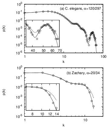
The sizes of all the four networks studied in this paper are larger than , and we have checked that Eqs. (2) and (5) give practically the same values of and are indistinguishable in the graphs. For much smaller networks, on the other hand, Eq. (2) actually predicts the degree distribution of sampled networks better than Eq. (5). In Fig. 3, we compare the simulation results for two small networks, the nematode C. elegans neural network YYAhn2005 with nodes and links and the Zachary karate club network Girvan2002 with nodes and links, with those two equations by substituting the original degree distribution , where is the number of nodes with degree . The figure clearly shows that Eq. (2) is more accurate.
The above equations turn out to be applied to the link sampling with the same sampling fraction as well. Here we can use the technique in Ref. Newman2005 to solve the bond percolation or epidemic model. Suppose a node, which originally had links before sampling, comes to have links. Because the random link sampling chooses links uniformly, the probability of the node having out of links is . Consequently the probability that a node in the sampled network has degree from all the possible original degree is , which leads us back to Eq. (5). The fact that those two sorts of sampling are described by the same equation is also supported by Fig. 2 showing the similar degree exponent changes for both node and link sampling.
As Stumpf et al. point out in Refs. Stumpf2005; Stumpf2005c, Eq. (5) for a power-law degree distribution yields deviation of from the original power-law form for quite small sampling fraction . For moderate values of , however, the deviation is not significant and we observe that the tangent of in the log-log plot actually becomes steeper from Eq. (5), consistent with our numerical observation about the node and link sampling as shown in Fig. 2. To extract the degree exponents from Eq. (5), first we calculate the degree distribution of the original networks by . Substituting that into Eq. (5), we obtain the degree distribution of the sampled networks corresponding to a given sampling fraction . The degree exponents from those in Fig. 2 show good agreement with the values from numerical simulation for both node and link sampling cases.

On the contrary, it is found that a degree exponent decreases for snowball sampling as we decrease the sampling fraction. By the definition of snowball sampling, hubs are more likely to be selected by this method. Furthermore, once a hub is picked, every node connected to the hub is selected in the next step unless it belongs to the previous layer. This characteristic of snowball sampling tends to conserve the degrees of easily selected hubs, which leads to the decrease of degree exponents by holding the “tail” of the power-law degree distribution. Figure 4 shows the degrees in a sampled network obtained by snowball sampling, and the nodes with large degree on the line clearly indicates a tendency to choose hubs and conserve their degrees. Therefore, the snowball sampling underestimates the degree exponent. In Ref. Clauset2004c, they show that the traceroute sampling can underestimate the degree exponent of a scale-free network by undersampling the low-degree nodes relative to the high-degree ones. In spite of the difference between the snowball and traceroute sampling, both of these methods overrepresent hubs and have the same “crawling” character used to identify the nodes. We infer that the decrease of degree exponents for both sampling methods is caused by these similar features.

We also check two closely related quantities, namely the average degree and the average path length (APL) in the sampled networks. APL is the average of shortest paths between all the pairs of nodes in a network, often used as a measure of network efficiency. In Fig. 5, we present APL of the giant component in the sampled networks obtained by the numerical simulation. For snowball sampling, APL decreases according to the decreased system size of sampled networks. On the other hand, for node and link sampling, the APL of a sampled network is larger than that of the original network for not-so-small sampling fraction, even though the size of the sampled network itself is smaller than the original one. As presented earlier, for node sampling, the number of links is proportional to the square of the number of the nodes, which leads to , where and are the numbers of links and nodes in a sampled network, respectively. This suggests that the average degree in a sampled network decreases as the sampling fraction becomes smaller. Obviously, for a given network, APL decreases as the average degree increases. The diminishment in the average degree, therefore, seems to have a stronger effect on APL than the overall system size in this case. Similar behavior of the average degree and APL is observed for link sampling, but in this case it seems that the “treelike” structure of sampled networks, related to the clustering coefficient discussed later, is responsible for that behavior.
III.2 Betweenness centrality distribution
Betweenness centrality (BC or load), which measures the centrality of a node by the traffic flow in a network, of node is defined as
| (6) |
where is the number of all the shortest pathways between a pair of nodes and is that of the shortest pathways running through a node KIGoh2002. It is known that the BC distribution follows a power-law for scale-free networks KIGoh2001; KIGoh2002.
Similar to the degree distribution, the BC distribution of sampled networks also follows power-law well as do the original networks. Figure 6 shows the change of the BC exponent, also obtained by Eq. (1), for each network and each sampling method. Similar to the degree exponent case, in general, BC exponents increase for node and link sampling and decrease for snowball sampling as the sampling fraction gets lower. Figure 6 bears a resemblance to Fig. 2 except for the case of arxiv.org, for which the BC exponent seems to be conserved for all the sampling methods. The correlation between degree and BC of nodes Barthelemy2003b, shown in Fig. 7, could explain the same direction of changes of degree and BC exponents. For assortative networks such as arxiv.org here, however, it is known that the degree-BC correlation is not clear KIGoh2003a, which explains the different behavior in Fig. 6(d). Therefore, at least empirically, we expect overestimation of a BC exponent by node and link sampling and underestimation by snowball sampling.


III.3 Assortativity
The assortativity , which measures the correlation between degrees of node linked to each other, is defined as the Pearson correlation coefficient of degrees between pairs of nodes Newman2002a. Positive values of stand for the positive degree-degree correlation which means that nodes with large degrees tend to be connected to one another. Most social networks have this positive degree correlation (assortative mixing), including the arxiv.org network considered in this paper. On the other hand, most biological and technological networks show negative degree correlation (disassortative mixing), including PIN and Internet AS network here. If there is no degree correlation among nodes (neutral), as in the case of BA model, the value of is in the vicinity of .


The change of assortativity for each network and each method is shown in Fig. 8. For node and link sampling, no noticeable changes of assortativity in the sampled networks are observed. Random choice of nodes or links appears to conserve assortativity well for these two methods. Sampled networks from snowball sampling, however, are shown to be more disassortative than the original networks. This pattern is common no matter whether the original network is assortative (arxiv.org), disassortative (PIN and Internet AS), or neutral (BA). In Ref. JDNoh2007a, a formula for the change of assortativity under the link sampling process is presented as follows,
| (7) |
where is the th moment of the degree of the original network. Our data fit perfectly well with Eq. (7), as shown in Fig. 9. In our datasets, where the degree exponent , dominates in Eq. (7) and in most cases, which is consistent with our numerical data for the link sampling.
There is another way to check the degree correlation, which is measuring the quantity , i.e., the average degree of nearest neighbors of nodes with degree Satorras2001b. Assortative mixing is represented by a positive slope of the graph, while the others by horizontal (neutral) or a negative slope (disassortative). Figure 10 shows the changes of these slopes for graphs of the sampled networks from two kinds of original networks by snowball sampling. The slope decreases, i.e., moves toward the negative value as the sampling fraction gets lower for both disassortative Internet AS and assortative arxiv.org.

We suggest that the more disassortative nature of sampled networks compared with the original ones is due to the last layer of snowball sampling method. In contrast to the conserved structure of the inner layers, a considerable number of links are lost for the nodes in the last layer. Meanwhile, hubs are likely to be selected for snowball sampling. This separation of “core” and “periphery” part is seen in Fig. 4, and the connections between hubs and nodes of the last layer can reduce the value of assortativity. The simulation shows that a sampled network containing the entire last layer is more disassortative than the one where only parts of the last layer are kept, which supports the hypothesis that the effect of the last layer induces disassortative mixing. Therefore, we have to be careful when measuring the assortativity for the network from the snowball sampling.
III.4 Clustering coefficient
The clustering coefficient of node is the ratio of the total number of the links connecting its nearest neighbors to the total number of all possible links between all these nearest neighbors Dorogovtsev2001a,
| (8) |
where is the degree of node . The clustering coefficient of a network is the average of this value over all the nodes , where is the number of nodes. Most real networks have much larger value of clustering coefficient than model networks such as ER or BA network due to, e.g., the community or modular structure.
In Fig. 11, we show the change of clustering coefficient for each original network and each sampling method. For node and snowball sampling, there is a little change of clustering coefficient depending on networks. On the other hand, link sampling prominently reduces the clustering coefficient. This effect is obvious since the random omission of links, the reverse process of link sampling, “opens up triangles fast” as stated in Ref. Kossinets2004. The link sampling, therefore, underestimates clustering coefficient of a network.

IV discussion and conclusions
| Degree | BC | Clustering | ||
|---|---|---|---|---|
| Exponent | Exponent | Assortativity | Coefficient | |
| Node | ||||
| Link | ||||
| Snowball |
In this paper, we have studied the changes of well-known quantities in complex networks for randomly sampled networks. Three kinds of sampling methods are applied, and three representative real-world networks, along with the BA model, are used as the original networks for numerical investigation. We have measured four typical quantities in sampled networks, which shows some characteristic patterns in changes of the quantities for each sampling method. Based on properties of sampling methods, possible explanations for such changes as well as the mathematical analysis are provided. We have also analyzed other networks than the scale-free ones such as Erdős-Rényi random network Erdos1959 and the growing network without the preferential attachment Barabasi1999, and the results show that the form of the degree distribution is conserved for the node and link sampling in those cases, consistent with the previous work Stumpf2005c.
Table 2 summarizes the results. To check the generality of the results, we also investigated the randomized version of each network in a similar fashion. The randomized networks were constructed by shuffling the links while conserving only the degree distribution Newman2002a. We found the same results with the original networks. The results in Table 2, therefore, seem to hold for scale-free networks in general and provide criteria for sampling method when some specific quantity is supposed to be investigated by the sampling. From another viewpoint, bias of some quantities can be predicted if a specific sampling method used to identify a network is known. If we are interested in the assortativity of a network, for example, node or link sampling can give fairly accurate values. For a clustering coefficient, on the other hand, the link sampling method should be avoided.
Sampling problems should be taken into account for real network research, but not much work has been done so far. Exploration of other characteristics of complex networks or using other sampling methods, rigorous analytic approaches, and establishing solid principles by more systematic investigation could all be important research topics for the future. We hope this work can make a contribution to this direction of research.
Acknowledgements.
We would like to thank Kwang-Il Goh for providing useful information, and appreciate Yong-Yeol Ahn for helping us with the link sampling formula. S.H.L. is grateful to Kim Bojeong Basic Science Foundation and KAIST for generous help. This work was supported by KOSEF through Grant No. R14-2002-059-01002-0 (P-J.K.) and by R01-2005-000-1112-0 (H.J.).References
- (1) M. E. J. Newman, SIAM Rev. 45, 167 (2003).
- (2) R. Albert and A.-L. Barabási, Rev. Mod. Phys. 74, 47 (2002).
- (3) S. N. Dorogovtsev and J. F. F. Mendes, Adv. Phys. 51, 1079 (2002); Evolution of Networks: From Biological Nets to the Internet and WWW (Oxford University Press, Oxford, 2003).
- (4) M. Faloutsos, P. Faloutsos, and C. Faloutsos, Comput. Commun. Rev. 29, 251 (1999).
- (5) H. Jeong, S. P. Mason, A.-L. Barabási, and Z. N. Oltvai, Nature (London) 411, 41 (2001).
- (6) M. E. J. Newman, Phys. Rev. E 64, 016131 (2001); 64, 016132 (2001).
- (7) E. Costenbader and T. W. Valente, Soc. Networks 25, 283 (2003).
- (8) G. Robins, P. Pattison, and J. Woolcock, Soc. Networks 26, 257 (2004).
- (9) G. Kossinets, cond-mat/0306335 (unpublished).
- (10) T. Petermann and P. De Los Rios, Eur. Phys. J. B 38, 201 (2004).
- (11) A. Clauset and C. Moore, Phys. Rev. Lett. 94, 018701 (2005).
- (12) D. Achlioptas, A. Clauset, D. Kempe, and C. Moore, cond-mat/0503087 (unpublished).
- (13) L. Dall’Asta, I. Alvarez-Hamelin, A. Barrat, A. Vázquez, and A. Vespignani, Phys. Rev. E 71, 036135 (2005).
- (14) M. P. H. Stumpf, C. Wiuf, and R. M. May, Proc. Natl. Acad. Sci. USA 102, 4221 (2005).
- (15) J. Scholz, M. Dejori, M. Stetter, and M. Greiner, Physica A 350, 622 (2005).
- (16) J.-D. J. Han, D. Dupuy, N. Bertin, M. E. Cusick, and M. Vidal, Nat. Biotechnol. (London) 23, 839 (2005).
- (17) M. Stumpf and C. Wiuf, Phys. Rev. E 72, 036118 (2005).
- (18) The traceroute command sends data packets toward a certain destination on the Internet, and one collects the traversed nodes and discovered paths during the process. Using such processes repeatedly, the sampled networks of the whole Internet are contructed at the AS or routers level.
- (19) K.-I. Goh, B. Kahng, and D. Kim, Phys. Rev. Lett. 87, 278701 (2001).
- (20) K.-I. Goh, E. Oh, H. Jeong, B. Kahng, and D. Kim, Proc. Natl. Acad. Sci. USA 99, 12583 (2002).
- (21) D. J. Watts and S. H. Strogatz, Nature (London) 393, 440 (1998).
- (22) A.-L. Barabási and R. Albert, Science 286, 509 (1999).
- (23) P. L. Krapivsky and S. Redner, Phys. Rev. E 63, 066123 (2001).
- (24) R. Albert, H. Jeong, and A-L. Barabási, Nature (London) 406, 378 (2000).
- (25) R. Cohen, K. Erez, D. ben-Avraham, and S. Havlin, Phys. Rev. Lett. 85, 4626 (2000).
- (26) R. Cohen, K. Erez, D. ben-Avraham, and S. Havlin, Phys. Rev. Lett. 86, 3682 (2001).
- (27) L. K. Gallos, R. Cohen, P. Argyrakis, A. Bunde, and S. Havlin, Phys. Rev. Lett. 94, 188701 (2005).
- (28) M. E. J. Newman, Phys. Rev. Lett. 89, 208701 (2002).
- (29) We verifed this relation by numerical simulation.
- (30) The term snowball sampling is from Steven K. Thomson, Sampling (John Wiley & Sons, Inc., New York, 2002).
- (31) M. E. J. Newman, Soc. Networks 25, 83 (2003).
- (32) C. Song, S. Havlin, and H. A. Makse, Nature (London) 433, 392 (2005).
- (33) K.-I. Goh, B. Kahng, and D. Kim, J. Korean Phys. Soc. 46, 551 (2005).
- (34) D. Meyer, University of Oregon Route Views Archive Project, http://archive.routeviews.org
- (35) M. E. J. Newman, Contemp. Phys. 46, 323 (2005).
- (36) M. E. J. Newman, Phys. Rev. Lett. 95, 108701 (2005).
- (37) Y.-Y. Ahn, B. J. Kim, and H. Jeong, Physica A 367, 531 (2006).
- (38) M. Girvan and M. E. J. Newman, Proc. Natl. Acad. Sci. USA 99, 7821 (2002).
- (39) M. Barthélemy, Eur. Phys. J. B 38, 163 (2004).
- (40) K.-I. Goh, E. Oh, B. Kahng, and D. Kim, Phys. Rev. E 67, 017101 (2003).
- (41) J. D. Noh, Phys. Rev. E 76, 026116 (2007).
- (42) R. Pastor-Satorras, A. Vázquez, and A. Vespignani, Phys. Rev. Lett. 87, 258701 (2001).
- (43) P. Erdős and A. Rényi, Publ. Math. (Debrecen) 6, 290 (1959).