August 11, 2026

Asymptotics of Toeplitz Determinants and the Emptiness Formation Probability for the XY Spin Chain

Fabio Franchini and Alexander G. Abanov Note: E-mail: Fabio.Franchini@sunysb.edu; Alexandre.Abanov@sunysb.edu Affiliation: Physics & Astronomy Department,
Stony Brook University,
Stony Brook, New York 11794-3800

Abstract

We study an asymptotic behavior of a special correlator known as the Emptiness Formation Probability (EFP) for the one-dimensional anisotropic XY spin-1/2 chain in a transverse magnetic field. This correlator is essentially the probability of formation of a ferromagnetic string of length $n$ in the antiferromagnetic ground state of the chain and plays an important role in the theory of integrable models. For the XY Spin Chain, the correlator can be expressed as the determinant of a Toeplitz matrix and its asymptotical behaviors for $n\to\infty$ throughout the phase diagram are obtained using known theorems and conjectures on Toeplitz determinants. We find that the decay is exponential everywhere in the phase diagram of the XY model except on the critical lines, i.e. where the spectrum is gapless. In these cases, a power-law prefactor with a universal exponent arises in addition to an exponential or Gaussian decay. The latter Gaussian behavior holds on the critical line corresponding to the isotropic XY model, while at the critical value of the magnetic field the EFP decays exponentially. At small anisotropy one has a crossover from the Gaussian to the exponential behavior. We study this crossover using the bosonization approach.

Keywords:

Emptiness Formation Probability, Integrable Models, XY Spin Chain, Toeplitz Determinants, Fisher-Hartwig Conjecture

pacs

75.10.Pq , 02.30.Ik , 02.30.Tb , 03.70.+k

I Introduction

Although the Bethe Ansatz bethe; yangyang; korepin93 gives us important information about the ground state and thermodynamics of quantum integrable one-dimensional models, the calculation of correlation functions for these models is still an open problem. Considerable progress, however, has been made recently in this field (see korepin93; jimbo and references therein).

Two main approaches express correlation functions in integrable models in terms of determinants of Fredholm operators korepin93; korepin94 or as multiple integrals jimbo. These expressions are exact but are very complex.

It was argued korepin93 that the simplest of the correlators in some integrable models is the so-called ”Emptiness Formation Probability” (EFP). For an XYZ spin chain in a magnetic field which is defined as

H=\sum_{i=1}^{N}\left[J_{x}\sigma_{i}^{x}\sigma_{i+1}^{x}+J_{y}\sigma_{i}^{y}\sigma_{i+1}^{y}+J_{z}\sigma_{i}^{z}\sigma_{i+1}^{z}\right]-h\sum_{i}\sigma_{i}^{z},

(1)

the Emptiness Formation Probability represents the ”Probability of Formation of Ferromagnetic Strings”

P(n)\equiv{1\over Z}\mbox{Tr}\,\left\{{\rm e}^{-\frac{H}{T}}\prod_{j=1}^{n}{1-\sigma_{i}^{z}\over 2}\right\},

(2)

where $Z\equiv\mbox{Tr}\,\left\{{\rm e}^{-H/T}\right\}$ . At zero temperature $T=0$ it becomes

P(n)\equiv\langle 0|\prod_{i=1}^{n}{1-\sigma_{i}^{z}\over 2}|0\rangle,

(3)

that is, the probability that $n$ consecutive spin sites are all found aligned downward in the ground state $|0\rangle$ .

It is conceivable that the study of this simple correlator will bring insights helpful to carry on the investigation of other correlators. But despite the fact that the EFP is the simplest of the correlators and despite considerable efforts devoted over the years to its study, there is still no easy recipe for its calculation (see, for instance, korepin93 – KLNS-2002). However, some progress has been achieved in finding an asymptotic behavior of $P(n)$ at large distances $n\rightarrow\infty$ .

For the XXZ spin chain in zero magnetic field ( $J_{x}=J_{y}$ , $h=0$ in (1)), the EFP is found to be Gaussian $P(n)\sim e^{-\alpha n^{2}}$ as $n\to\infty$ in the critical regime $|J_{z}|<|J_{x}|$ at zero temperature and exponential $e^{-\beta n}$ at finite temperature (KMST_gen-2002,KLNS-2002).

A qualitative argument in favor of Gaussian decay was given in Ref. abanovkor within a field theory approach. It was argued there that the asymptotics of the EFP are defined by the action of an optimal fluctuation (instanton) corresponding to the EFP. In the critical model, this fluctuation will have a form of a “ $n\times n$ ” droplet in space-time with the area $A\sim n^{2}$ and the corresponding action $S\approx\alpha n^{2}$ which gives the decay $P(n)\sim e^{-\alpha n^{2}}$ . Similarly, at finite temperature the droplet becomes rectangular (one dimension $n$ is replaced by an inverse temperature $T^{-1}$ ) and the action cost is proportional to $n$ , giving $P(n)\sim e^{-\beta n}$ . This argument is based on the criticality of the theory¹¹ 1 More precisely, on the assumption that temporal and spatial dimensions of an instanton scale similarly. and it is interesting to consider whether it could be extended to a non-critical theory. A naïve extension of the argument would give the optimal fluctuation with space-time dimensions $n\times\xi$ where $\xi$ is a typical correlation length (in time) of the theory. This would result in $P(n)\sim e^{-\beta n}$ for non-critical theories, similarly to the case of finite temperature in critical regime. The rate of decay $\beta$ would be proportional to the correlation length of the theory.

In this paper we examine the relation between the asymptotic behavior of the EFP and criticality using the example of the Anisotropic XY spin-1/2 chain in a transverse magnetic field

H=\sum_{i=1}^{N}\left[\left({1+\gamma\over 2}\right)\sigma_{i}^{x}\sigma_{i+1}^{x}+\left({1-\gamma\over 2}\right)\sigma_{i}^{y}\sigma_{i+1}^{y}\right]-h\sum_{i=1}^{N}\sigma_{i}^{z},

(4)

where $\sigma_{i}^{\alpha}$ , with $\alpha=x,y,z$ , are the Pauli matrices which describe spin operators on the $i$ -th lattice site of the spin chain and, for definiteness, we require periodic boundary conditions: $\sigma_{i}^{\alpha}=\sigma_{i+N}^{\alpha}$ ( $N>>1$ ). This model is, probably, the simplest model that has both critical and non-critical regimes in its $\gamma-h$ phase diagram.

Using the mapping of the model (4) to free one-dimensional fermions (Jordan-Wigner transformation) one can express the EFP $P(n)$ of this system in terms of a determinant of a $n\times n$ Toeplitz matrix. The asymptotic behavior of these matrices can be found using known theorems from the theory of Toeplitz determinants. This approach and technique is exactly the one of Ref. mccoy, where it was used to find the spin-spin correlation functions for the model (4). This technique was also used in Ref. shiroishi for the EFP in the case of the Isotropic XY model (Eq. (4) with $\gamma=0$ ). In the latter work it was shown that the EFP decays in a Gaussian way for the critical theory ( $\gamma=0$ , $-1\leq h\leq 1$ ). This case corresponds to one of the two critical lines in the $\gamma-h$ phase diagram of the model (4). The other line is the critical magnetization line(s) ( $h=\pm 1$ ). In the rest of the two-dimensional $\gamma-h$ phase diagram, the model is non-critical.

We obtain that the EFP is asymptotically exponential in most of the phase diagram according to the naïve expectations and that it is Gaussian only at $\gamma=0$ in agreement with previous works on XXZ spin chains and Ref. shiroishi. However, on the critical lines $h=\pm 1$ , in addition to the exponential decay, a pre-exponential power-law factor arises, with a universal exponent. The power-law prefactor is present in the isotropic case as well, but with a different exponent.

The paper is organized in the following way: we briefly review the phase diagram of the XY Spin-1/2 Chain in Section II. In Section III we explain how one can express the EFP as the determinant of a Toeplitz matrix and review our results so that readers who are not interested in derivations can skip the next sections. In Section IV we analyze the exponential decay of the EFP for the non-critical and critical phases of the anisotropic XY Model. In Section V we derive in detail the asymptotic behaviors, including the pre-exponential factors, of both non-critical and critical parts of the phase diagram. In Section VI we study a special line of the phase diagram on which the ground state is known exactly and compare the explicit results one can obtain using the exact ground state with the asymptotes of the EFP we derived in the previous sections. In Section VII we report on the already known results for the EFP of the isotropic XY model shiroishi. In Section VIII we make contact with Ref. abanovkor using a bosonization approach to discuss the crossover as a function of $n$ from the Gaussian to the exponential behavior of EFP for the case of small anisotropy $\gamma$ . Finally, Section IX will summarize our results. For the reader’s convenience we collect some results on asymptotic behavior of Toeplitz determinants which are extensively used in the rest of the paper in the first appendix. The second appendix presents the analysis of the finite temperature behavior of the EFP, which gives an expected exponential decay. The third appendix gives some mathematical details on the calculation of the stationary action in the bosonization approach of Section VIII.

Some of the results presented in this paper have been announced in a previous letter abanovfran without details, which will be given here.

II The Anisotropic XY Model

The XY spin model defined by (4) has been solved in LSM-1961 in the case of zero magnetic field and in mccoy in the presence of a magnetic field. We follow the standard prescription LSM-1961 and reformulate the Hamiltonian (4) in terms of spinless fermions $\psi_{i}$ by means of a Jordan-Wigner transformation:

	$\displaystyle\sigma_{j}^{+}$	$\displaystyle=$	$\displaystyle\psi_{j}^{\dagger}{\rm e}^{{\rm i}\pi\sum_{k<i}\psi_{k}^{\dagger}\psi_{k}}=\psi_{j}^{\dagger}\prod_{k<j}\left(2\psi_{k}^{\dagger}\psi_{k}-1\right),$		(5)
	$\displaystyle\sigma_{j}^{z}$	$\displaystyle=$	$\displaystyle 2\psi_{j}^{\dagger}\psi_{j}-1,$		(6)

where, as usual, $\sigma^{\pm}=(\sigma^{x}\pm i\sigma^{y})/2$ :

H=\sum_{i=1}^{N}\left(\psi_{i}^{\dagger}\psi_{i+1}+\psi_{i+1}^{\dagger}\psi_{i}+\gamma\;\psi_{i}^{\dagger}\psi_{i+1}^{\dagger}+\gamma\;\psi_{i+1}\psi_{i}-2h\;\psi_{i}^{\dagger}\psi_{i}\right).

(7)

In Fourier components $\psi_{j}=\sum_{q}\psi_{q}{\rm e}^{{\rm i}qj}$ , we have:

H=\sum_{q}\left[2\left(\cos\!q-h\right)\psi_{q}^{\dagger}\psi_{q}+{\rm i}\gamma\sin\!q\>\psi_{q}^{\dagger}\psi_{-q}^{\dagger}-{\rm i}\gamma\sin\!q\>\psi_{-q}\psi_{q}\right].

(8)

The Bogoliubov transformation

\chi_{q}=\cos\!{\vartheta_{q}\over 2}\>\psi_{q}+{\rm i}\sin\!{\vartheta_{q}\over 2}\>\psi_{-q}^{\dagger}

(9)

with “rotation angle” $\vartheta_{q}$

e^{i\vartheta_{q}}=\frac{1}{\varepsilon_{q}}(\cos q-h+i\gamma\sin q),

(10)

brings the Hamiltonian (8) to the diagonal form $\sum_{q}\varepsilon_{q}\chi_{q}^{\dagger}\chi_{q}$ with the quasiparticle spectrum

\varepsilon_{q}=\sqrt{\left(\cos q-h\right)^{2}+\gamma^{2}\sin^{2}q}.

(11)

We recognize from (11) that the theory is critical, i.e. gapless, for $h=\pm 1$ or for $\gamma=0$ and $|h|<1$ .

In Fig. 1 we show the phase diagram of the XY model, which has obvious symmetries $\gamma\to-\gamma$ and $h\to-h$ . However, the latter is not a symmetry of the EFP. Therefore, we show only the part of the diagram corresponding to $\gamma\geq 0$ . The phase diagram has both critical and non-critical regimes. Three critical lines $\Omega_{0}$ (Isotropic XY model: $\gamma=0$ , $|h|<1$ ) and $\Omega_{\pm}$ (critical magnetic field: $h=\pm 1$ ) divide the phase diagram into three non-critical domains, $\Sigma_{-}$ , $\Sigma_{0}$ , and $\Sigma_{+}$ ( $h<-1$ , $-1<h<1$ , and $h>1$ respectively). Fig. 1 also shows the line $\gamma=1$ ( $\Gamma_{I}$ ) corresponding to the Ising model in transverse magnetic field and the line $\gamma^{2}+h^{2}=1$ ( $\Gamma_{E}$ ) on which the wave function of the ground state is factorized into a product of single spin states shrock (we will consider this line in detail in Section VI).

Refer to caption — Figure 1: Phase diagram of the XY Model (only the part $\gamma\geq 0$ is shown). The theory is critical for $h=\pm 1$ ( $\Omega_{\pm}$ ) and for $\gamma=0$ and $|h|<1$ ( $\Omega_{0}$ ). The line $\Gamma_{I}$ represents the Ising Model in transverse field. On the line $\Gamma_{E}$ the ground state of the theory is a product of single spin states.

The fermionic correlators are easy to obtain from (8). In the thermodynamic limit they read LSM-1961; mccoy

	$\displaystyle F_{jk}$	$\displaystyle\equiv$	$\displaystyle{\rm i}\langle\psi_{j}\psi_{k}\rangle=-{\rm i}\langle\psi_{j}^{\dagger}\psi_{k}^{\dagger}\rangle=\int_{0}^{2\pi}{{\displaystyle\rm\mathstrut d}q\over 2\pi}\;\frac{1}{2}\sin\vartheta_{q}{\rm e}^{{\rm i}q(j-k)},$		(12)
	$\displaystyle G_{jk}$	$\displaystyle\equiv$	$\displaystyle\langle\psi_{j}\psi_{k}^{\dagger}\rangle=\int_{0}^{2\pi}{{\displaystyle\rm\mathstrut d}q\over 2\pi}\;\frac{1+\cos\vartheta_{q}}{2}{\rm e}^{{\rm i}q(j-k)}.$		(13)

III Emptiness Formation Probability in the XY model

We are mostly interested in the value of the correlator (2) at zero temperature (the non-zero temperature case is deferred to the second appendix). In terms of spinless fermions, one can express the EFP (3) as the expectation value over the ground state of the theory shiroishi

P(n)=\langle\prod_{j=1}^{n}\psi_{j}\psi_{j}^{\dagger}\rangle.

(14)

This expression projects the ground state on a configuration without particles on a string of length $n$ and gives the meaning to the name “Emptiness Formation Probability”.

Let us introduce the $2n\times 2n$ skew-symmetric matrix ${\bf M}$ of correlation functions

{\bf M}=\pmatrix{{-{\rm i}\bf F}&{\bf G}\cr-{\bf G}&{\rm i}{\bf F}\cr},

(15)

where ${\bf F}$ and ${\bf G}$ are $n\times n$ matrices with matrix elements given by $F_{jk}$ and $G_{jk}$ from (12,13) respectively. Then, using Wick’s theorem on the r.h.s of (14), we obtain

P(n)={\rm Pf}({\bf M}).

(16)

The Pfaffian mehta2 is defined as

{\rm Pf}({\bf M})\equiv\sum_{P}(-1)^{P}M_{p_{1}p_{2}}M_{p_{3}p_{4}}\ldots M_{p_{2n-1}p_{2n}},

(17)

where $P=\{p_{1},p_{2},\ldots,p_{2n}\}$ is a permutation of $\{1,2,\ldots,2n\}$ , the sum is performed over all possible permutations, and $(-1)^{P}$ is the parity of the permutation. Using one of the properties of the Pfaffian we have

P(n)={\rm Pf}({\bf M})=\sqrt{\det({\bf M})}.

(18)

We perform a unitary transformation

{\bf M^{\prime}}={\bf UMU}^{\dagger}=\pmatrix{0&{\bf S_{n}}\cr-{\bf S_{n}}^{\dagger}&0\cr},\qquad{\bf U}={1\over\sqrt{2}}\pmatrix{{\bf I}&{\bf-I}\cr{\bf I}&{\bf I}\cr},

(19)

where ${\bf I}$ is a unit $n\times n$ matrix and ${\bf S_{n}}={\bf G}+{\rm i}{\bf F}$ and ${\bf S_{n}}^{\dagger}={\bf G}-{\rm i}{\bf F}$ . This allows us to calculate the determinant of ${\bf M}$ as

\det({\bf M})=\det({\bf M^{\prime}})=\det({\bf S_{n}})\cdot\det({\bf S_{n}}^{\dagger})=\left|\det({\bf S_{n}})\right|^{2}.

(20)

The matrix ${\bf S_{n}}$ is a $n\times n$ Toeplitz matrix (i.e. its matrix elements depend only on the difference of row and column indices basor). The generating function $\sigma(q)$ of a Toeplitz matrix is defined by

({\bf S_{n}})_{jk}=\int_{0}^{2\pi}{dq\over 2\pi}\;\sigma(q){\rm e}^{{\rm i}q(j-k)}

(21)

and in our case can be found from (12,13) as

\sigma(q)={1\over 2}\left(1+{\rm e}^{{\rm i}\vartheta_{q}}\right)={1\over 2}+{\cos q-h+{\rm i}\gamma\sin q\over 2\sqrt{(\cos q-h)^{2}+\gamma^{2}\sin^{2}q}}.

(22)

Thus, the problem of calculation of the EFP

P(n)=\left|\det({\bf S_{n}})\right|,

(23)

is reduced (exactly) to the calculation of the determinant of the $n\times n$ Toeplitz matrix ${\bf S_{n}}$ defined by the generating function (21,22). The representation (23) is exact and valid for any $n$ . In our study we are interested in finding an asymptotic behavior of (23) at large $n\to\infty$ . ²² 2 The reader might notice that our generating function (22) is almost the same as the one analyzed by Barouch et al. in mccoy ( $\sigma_{[13]}(q)={\cos q-h+{\rm i}\gamma\sin q\over\sqrt{(\cos q-h)^{2}+\gamma^{2}\sin^{2}q}}$ ). The only difference is the shift by the unity in our expression. This difference changes dramatically the analytical structure of the generating function, in particular, its winding number around the origin, and requires a new analysis of the generated Toeplitz determinants.

Most of these results are derived using known theorems on the asymptotic behavior of Toeplitz determinants. We collect these theorems in Appendix A. In the following sections we apply them to extract the corresponding asymptotes of $P(n)$ at $n\to\infty$ in the different regions of the phase diagram. Two major distinctions have to be made in this process. For the critical isotropic ( $\gamma=0$ ) XY model, one applies what is known as Widom’s Theorem and one finds a Gaussian behavior with a power law prefactor shiroishi. In the rest of the phase diagram, we apply different formulations of what is known in general as the Fisher-Hartwig conjecture, which always leads to an exponential asymptotic behavior. As expected, we find a pure exponential decay for the EFP in the non-critical regions.

For $h>1$ , the exponential decay is modulated by an additional oscillatory behavior.

At the critical magnetizations $h=\pm 1$ , we discover an exponential decay with a power law pre-factor. Moreover, by extending the existing theorems on Toeplitz determinants beyond their range of applicability, for $h=\pm 1$ we obtain the first order corrections to the asymptotics as a faster decaying power law with the same exponential factor. For $h=1$ , the first order correction is also oscillating and this means that the EFP presents an oscillatory behavior of the EFP for $h\geq 1$ .

The reader who is not interested in the mathematical details of our derivations can find the results in Table 1 and skip the following sections to go directly to Sec. VIII, where we analyze the crossover between the Gaussian behavior at $\gamma=0$ and the asymptotic exponential decay at finite $\gamma$ using a bosonization approach.

EFP for the Anisotropic XY model
Region	$\gamma$ , $h$	$P(n)$	Eq.	Section	Theorem
$\Sigma_{-}$	$h<-1$	$E\,{\rm e}^{-n\beta}$	42	V.1.1	Szegö
$\Sigma_{0}$	$-1<h<1$	$E\,{\rm e}^{-n\beta}$	42	V.1.2	FH
$\Sigma_{+}$	$h>1$	${\it E}\left[1+(-1)^{n}A\right]\>{\rm e}^{-n\beta}$	56	V.1.3	gFH
$\Gamma_{E}$	$\gamma^{2}+h^{2}=1$	$E\,{\rm e}^{-n\beta}$	87	VI	Exact
${\bf\Omega_{+}}$	$h=1$	${\it E}\>n^{-{1/16}}\left[1+(-1)^{n}A/\sqrt{n}\>\right]\>{\rm e}^{-n\beta}$	71	V.2.1	gFH
${\bf\Omega_{-}}$	$h=-1$	${\it E}\>n^{-{1/16}}\left[1+A/\sqrt{n}\>\right]\>{\rm e}^{-n\beta}$	82	V.2.2	gFH
${\bf\Omega_{0}}$	$\gamma=0$ , $\|h\|<1$	$E\,n^{-1/4}e^{-n^{2}\alpha}$	89	VII	Widom

Table 1: Asymptotic behavior of the EFP in different regimes. The exponential decay rate

\beta

is given by Eq. (25) for all regimes. The regions in boldface are the critical ones. The coefficients

E,A

are functions of

h

and

\gamma

whose explicit expressions are provided in the text. Relevant theorems on Toeplitz determinants are collected in the A.

IV Singularities of $\sigma(q)$ and exponential behavior of the EFP

To derive the asymptotic behavior of the EFP we rely on the theorems on determinants of Toeplitz matrices. These theorems depend greatly on the analytical structure of the generating function (22), especially on its zeros and singularities.

Setting $\gamma=0$ in (22), we see that for the Isotropic XY model the generating function has only a limited support within its period $[0,2\pi]$ . This case is covered by what is known as Widom’s Theorem and will be considered in Section VII.

In the remaining parts of the phase-diagram the generating function has only pointwise singularities (zeros) as it is shown in Fig. 2. These cases are treated under a general (not yet completely proven) conjecture known as the Fisher-Hartwig conjecture (FH), which prescribes the leading asymptotic behavior of the Toeplitz determinant to be exponential in $n$ :

P(n){\stackrel{{\scriptstyle n\rightarrow\infty}}{{\sim}}}{\rm e}^{-\beta n}.

(24)

While the pre-exponential factors depend upon the particulars of the singularities of the generating function, the exponential decay rate is given in the whole phase diagram ( $\gamma\neq 0$ ) according to FH as

	$\displaystyle\beta(h,\gamma)$	$\displaystyle=$	$\displaystyle-\int_{0}^{2\pi}{{\displaystyle\rm\mathstrut d}q\over 2\pi}\;\log\left\|\sigma(q)\right\|$		(25)
		$\displaystyle=$	$\displaystyle-\int_{0}^{\pi}{{\displaystyle\rm\mathstrut d}q\over 2\pi}\;\log\left[{1\over 2}\left(1+{\cos q-h\over\sqrt{\left(\cos q-h\right)^{2}+\gamma^{2}\sin^{2}q}}\right)\right].$		(25)

The integral in (25) is convergent for all $h$ and all $\gamma\neq 0$ and $\beta(h,\gamma)$ is a continuous function of its parameters.

In Fig. 3, $\beta(h,\gamma)$ is plotted as a function of $h$ at several values of $\gamma$ . One can see that $\beta(h,\gamma)$ is continuous but has weak (logarithmic) singularities at $h=\pm 1$ . This is one of the effects of the criticality of the model on the asymptotic behavior of EFP.

These weak singularities are also a manifestation of the rich analytical structure underlying $\beta(h,\gamma)$ and the generating function (22). To understand these structures, we interpret the periodic generating function (22) as the restriction to the unit circle ( $z={\rm e}^{{\rm i}\theta}$ ) of the complex function

\sigma(z)\equiv{1\over 2}\left(1+{p_{1}(z)\over\sqrt{p_{1}(z)\cdot p_{2}(z)}}\right),

(26)

where

	$\displaystyle p_{1}(z)={1+\gamma\over 2z}(z-z_{1})(z-z_{2}),$		(27)
	$\displaystyle p_{2}(z)={1+\gamma\over 2z}(z_{1}z-1)(z_{2}z-1)$		(28)

with

	$\displaystyle z_{1}={h-\sqrt{h^{2}+\gamma^{2}-1}\over 1+\gamma},$		(29)
	$\displaystyle z_{2}={h+\sqrt{h^{2}+\gamma^{2}-1}\over 1+\gamma}.$		(30)

The integral in (25) can be regarded as a contour integral over the unit circle of the function (26). We can deform the contour of integration taking into account the complex structure of the integrand in the various regions (see Fig. 4) and express (25) as a simpler integral on the real axis (after partial integration and some algebra).

IV.1 The non-critical regions ( $\Sigma_{\pm}$ and $\Sigma_{0}$ )

IV.1.1 $\Sigma_{-}$ ( $h<-1$ )

For $h<-1$ , the analytical structure of the integrand of (25) is shown in Fig. 4a. We re-write the decay rate (25) in this region as

\beta(h,\gamma)={1\over 2}\ln\left[{\sqrt{h^{2}+\gamma^{2}-1}-h\over\gamma+1}\right]-\Lambda(h,\gamma)-\Delta(h,\gamma),

(31)

where

	$\displaystyle\Lambda(h,\gamma)$	$\displaystyle\equiv$	$\displaystyle\ln\left\|{1\over 2}\left(1-{h\over\|h\|}\sqrt{{1-\gamma\over 1+\gamma}}\right)\right\|,$		(32)
	$\displaystyle\Delta(h,\gamma)$	$\displaystyle\equiv$	$\displaystyle\int^{1}_{\|K\|}{{\displaystyle\rm\mathstrut d}x\over 2\pi}{1\over\sqrt{(1-x^{2})(x^{2}-K^{2})}}\left(x+{K\over x}\right)\ln\left\|{x-a\over x+a}\right\|$		(33)

with

	$\displaystyle K$	$\displaystyle\equiv$	$\displaystyle{\sqrt{h^{2}+\gamma^{2}-1}-\gamma\over\sqrt{h^{2}+\gamma^{2}-1}+\gamma},$		(34)
	$\displaystyle a$	$\displaystyle\equiv$	$\displaystyle{\sqrt{h^{2}+\gamma^{2}-1}-\gamma\over h-1}.$		(35)

This decomposition of $\beta(h,\gamma)$ is especially useful in analyzing the transitions between non-critical and critical regimes. In fact, we will see that the functions $\Lambda(h,\gamma)$ and $\Delta(h,\gamma)$ defined above are universal across the phase diagram (hence the need for the seemingly redundant absolute values in our definitions).

IV.1.2 $\Sigma_{0}$ ( $|h|<1$ )

As before, we can express the contour integral defining $\beta(h,\gamma)$ as a standard integral on the real axis. For $|h|<1$ and $h^{2}+\gamma^{2}>1$ , the structure of the integrand is depicted in Fig. 4c and the decay rate is simply

\beta(h,\gamma)=-\Lambda(h,\gamma)-\Delta(h,\gamma),

(36)

where $\Lambda(h,\gamma)$ and $\Delta(h,\gamma)$ have already been defined in (32,33).

For $h^{2}+\gamma^{2}<1$ , the structure is quite different (see Fig. 4d). In this region the expression for $\beta(h,\gamma)$ in terms of a real axis integral is complicated and will therefore be omitted it in this paper.

IV.1.3 $\Sigma_{+}$ ( $h>1$ )

A calculation similar to the previous ones (see Fig. 4f) gives the expression for the decay factor for $h>1$ :

\beta(h,\gamma)={1\over 2}\ln\left[{\sqrt{h^{2}+\gamma^{2}-1}+h\over\gamma+1}\right]-\Lambda(h,\gamma)-\Delta(h,\gamma),

(37)

where $\Lambda(h,\gamma)$ and $\Delta(h,\gamma)$ were introduced in (32) and (33).

One important difference exists in this region: as will be discussed in length later in Section V.1.3, in $\Sigma_{+}$ there are two equivalent representations of the generating function. This ambiguity reflects on the value of $\beta$ , in that the choice of the representation for the generating function determines the branch cuts in Fig. 4. We will see that we have to use both values of $\beta$ , which differ only by an imaginary constant:

\beta^{\prime}=\beta+{\rm i}\pi

(38)

and this will add an oscillatory behavior to the EFP.

IV.2 The critical lines ( $\Omega_{\pm}$ )

We can calculate the decay factor $\beta$ at $h=1$ ( $\Omega_{+}$ ) from a limiting procedure on (36) or (37). At $h=1$ , only $\Delta(h,\gamma)$ is nonvanishing, thus guaranteeing the continuity of $\beta$ across the critical line. From an appropriate limit of (33), we calculate the decay rate for $h=1$ as

\beta(1,\gamma)=-\int_{0}^{1}{{\displaystyle\rm\mathstrut d}x\over 2\pi}{1\over\sqrt{1-x^{2}}}\ln\left|{1-\gamma x\over 1+\gamma x}\right|-\ln\left|{1\over 2}\left(1-\sqrt{1-\gamma\over 1+\gamma}\right)\right|.

(39)

As discussed before in reference to (37), the definition of $\beta(1,\gamma)$ is not unique and, as in (38), will generate again an oscillatory behavior for the EFP (see later in Sec. V.2.1).

The value of $\beta$ at $h=-1$ can also be obtained from a limiting procedure on (33)

\beta(-1,\gamma)=\int_{0}^{1}{{\displaystyle\rm\mathstrut d}x\over 2\pi}{1\over\sqrt{1-x^{2}}}\ln\left|{1-\gamma x\over 1+\gamma x}\right|-\ln\left|{1\over 2}\left(1+\sqrt{1-\gamma\over 1+\gamma}\right)\right|.

(40)

As can be seen in Fig. 3, the decay factor $\beta$ is continuous across the critical lines, but has a discontinuity in its derivative. As $\beta$ approaches the critical lines, it actually shows a non-analytical behavior leading to a logarithmic singularity:

\beta(h=\pm 1+\epsilon,\gamma)=\beta(\pm 1,\gamma)+{\gamma\over\pi}\;\epsilon\ln|\epsilon|.

(41)

The derivative $d\beta/dh$ diverges logarithmically as $h\to\pm 1$ .

Moreover, one can easily notice from the difference between expression (36) and (37) that even the finite part of the derivative of $\beta(h,\gamma)$ by $h$ is different if one approaches the critical line $h=1$ from above or below, due to the appearance of the additional term in (37). The same holds across the critical line $h=-1$ , due to the presence of the first term in (31), which doesn’t appear in (36).

V The pre-exponential factors

For $\gamma\neq 0$ , the leading behavior of the EFP is always exponential. However, the singularities of the generating function are different in different regions of the phase diagram and we must therefore use different forms of the Fisher-Hartwig conjecture in order to derive the pre-exponential factors and determine the asymptotic behavior of $P(n)$ . We will now show how to obtain the results for each of the regions.

V.1 The non-critical regions ( $\Sigma_{\pm}$ and $\Sigma_{0}$ )

V.1.1 $\Sigma_{-}$ ( $h<-1$ )

In this region ( $\gamma\neq 0$ , $h<-1$ ) the generating function (22) is nonzero for all $q$ (see Fig. 2a): this is the simplest case and can be treated using the (rigorously proven) Strong Szegö Limit Theorem, see (97). It gives

P(n)=\left|\det({\bf S_{n}})\right|{\stackrel{{\scriptstyle n\rightarrow\infty}}{{\sim}}}{\it E_{-}}(h,\gamma){\rm e}^{-\beta(h,\gamma)n}

(42)

with $\beta(h,\gamma)$ given by (25) or (31) and

{\it E_{-}}(h,\gamma)=\exp\left(\sum_{k=1}^{\infty}k\hat{\sigma}_{k}\hat{\sigma}_{-k}\right),

(43)

where $\hat{\sigma}_{k}$ is defined in (99) as the $k$ -th Fourier component of the logarithm of $\sigma$ :

	$\displaystyle\hat{\sigma}_{k}$	$\displaystyle\equiv$	$\displaystyle\int_{0}^{2\pi}{{\displaystyle\rm\mathstrut d}q\over 2\pi}\;\left[\log\sigma(q)\right]{\rm e}^{-{\rm i}kq}$		(44)
		$\displaystyle=$	$\displaystyle\int_{0}^{2\pi}{{\displaystyle\rm\mathstrut d}q\over 2\pi}\;{\rm e}^{-{\rm i}kq}\log\left(1+{\cos q-h+{\rm i}\gamma\sin q\over\sqrt{\left(\cos q-h\right)^{2}+\gamma^{2}\sin^{2}q}}\right).$		(44)

The sum in (43) is convergent only for $\gamma\neq 0$ and for $h<-1$ . For $h\geq-1$ , the generating function (22) develops singularities which produce $1/k$ contributions to (44) that make the sum in (43) divergent. Therefore, in the rest of the phase diagram these singularities have to be treated to absorb the harmonic series contributions. Consequently, each region of the phase diagram will involve a different definition for the pre-exponential factor and the ”regularization” procedure will sometimes generate an additional power-law contribution. The result is given by the Fisher-Hartwig conjecture that we must use in the remainder of the phase diagram.

V.1.2 $\Sigma_{0}$ ( $|h|<1$ )

As can be noticed from Fig. 2c, in $\Sigma_{0}$ ( $\gamma\neq 0$ , $-1<h<1$ ) the generating function $\sigma(q)$ vanishes and its phase has a discontinuity of $\pi$ at $q=\pi$ . The asymptotic behavior of Toeplitz determinants with this type of singularities in the generating function is given by FH, which is actually proven for cases in which only one singularity is present.

We decompose the generating function as in (100)

\sigma(q)=\tau(q){\rm e}^{{{\rm i}\over 2}[(q-\pi){\rm\>mod\>}2\pi-\pi]}\left(2-2\cos(q-\pi)\right)^{1/2}

(45)

and using (101) we obtain

P(n)=\left|\det({\bf S_{n}})\right|{\stackrel{{\scriptstyle n\rightarrow\infty}}{{\sim}}}{\it E_{0}}(h,\gamma)\>{\rm e}^{-\beta(h,\gamma)n}.

(46)

The behavior is exponential as before with the decay rate $\beta(h,\gamma)$ from (25,36), but the pre-exponential factor is different. According to (102) it is given by

{\it E_{0}}(h,\gamma)\equiv{E[\tau]\over\tau_{-}(\pi)},

(47)

where, as in (98) and (99)

\displaystyle E[\tau]

\displaystyle=

\displaystyle\exp\left(\sum_{k=1}^{\infty}k\hat{\tau}_{k}\hat{\tau}_{-k}\right)

(48)

and

\hat{\tau}_{k}=\hat{\sigma}_{k}-{(-1)^{k}\over k}\;\theta(k).

(49)

Here $\theta(k)$ is the usual Heaviside step function. As we mentioned in the previous section, $\hat{\sigma}_{k}$ (44) has $1/k$ contributions from singularities of $\sigma(q)$ and the effect of the parametrization (45) is to cure (remove) these harmonic series divergences of the prefactor of the EFP in this regime.

V.1.3 $\Sigma_{+}$ ( $h>1$ )

In $\Sigma_{+}$ ( $\gamma\neq 0$ , $h>1$ ), $\sigma(q)$ vanishes at $q=0$ and $q=\pi$ and its phase presents two $\pi$ jumps at those points (Fig. 2e).

In this case the application of FH leads to some ambiguity, because there exist two representations of the kind (100) and one obtains two values for $\beta(h,\gamma)$ using the two representations of the generating function: $\beta_{1}=\beta$ and $\beta_{2}=\beta+{\rm i}\pi$ , with $\beta$ from (25) or (37). This ambiguity is resolved by the (yet unproven) generalized Fisher-Hartwig conjecture (gFH), which gives EFP as a sum of two terms so that both values of $\beta$ ’s are used (see the appendix A.3 or basor).

The two leading inequivalent parametrizations (107) are:

$\displaystyle\sigma(q)$	$\displaystyle=$	$\displaystyle\tau^{1}(q){\rm e}^{{{\rm i}\over 2}[(q-\pi){\rm\>mod\>}2\pi-\pi]}\left(2-2\cos(q-\pi)\right)^{1/2}$	(51)
		$\displaystyle\qquad\times{\rm e}^{-{{\rm i}\over 2}[q{\rm\>mod\>}2\pi-\pi]}\left(2-2\cos q\right)^{1/2}$
	$\displaystyle=$	$\displaystyle\tau^{2}(q){\rm e}^{-{{\rm i}\over 2}[(q-\pi){\rm\>mod\>}2\pi-\pi]}\left(2-2\cos(q-\pi)\right)^{1/2}$
		$\displaystyle\qquad\times{\rm e}^{{{\rm i}\over 2}[q{\rm\>mod\>}2\pi-\pi]}\left(2-2\cos q\right)^{1/2}.$

Application of (108) gives the asymptotic behavior of the determinants as

\left|\det({\bf S_{n}})\right|{\stackrel{{\scriptstyle n\rightarrow\infty}}{{\sim}}}\left[{\it E^{1}_{+}}(h,\gamma)+(-1)^{n}{\it E^{2}_{+}}(h,\gamma)\right]\>{\rm e}^{-\beta(h,\gamma)n}

(52)

with

	$\displaystyle{\it E^{1}_{+}}(h,\gamma)\equiv{E[\tau]\over\tau_{+}(0)\tau_{-}(\pi)},$		(53)
	$\displaystyle{\it E^{2}_{+}}(h,\gamma)\equiv{E[\tau]\over\tau_{+}(\pi)\tau_{-}(0)}$		(54)

and $\beta(h,\gamma)$ , $E[\tau]$ defined in (25,48) with

\hat{\tau}_{k}=\hat{\sigma}_{k}-{(-1)^{k}\over k}\;\theta(k)-{1\over k}\;\theta(-k).

(55)

Once again, as in the previous section, the effect of the parametrization is to remove the $1/k$ contributions to $\hat{\sigma}_{k}$ (44) due to the singularities of the generating function.

We conclude that the non-critical theory presents an exponential asymptotic behavior of the EFP. In the region $\Sigma_{+}$ , however, the EFP in addition has even-odd oscillations

P(n){\stackrel{{\scriptstyle n\rightarrow\infty}}{{\sim}}}{\it E^{1}_{+}}(h,\gamma)\left[1+A_{+}(h,\gamma)\cos(\pi n)\right]\>{\rm e}^{-\beta(h,\gamma)n},

(56)

where the exponential decay factor is given by (37).

The amplitude of the oscillations is

$\displaystyle A_{+}(h,\gamma)$	$\displaystyle\equiv$	$\displaystyle{\tau_{+}(0)\tau_{-}(\pi)\over\tau_{-}(0)\tau_{+}(\pi)}$	(57)
	$\displaystyle=$	$\displaystyle{\tau(0)\over\tau(\pi)}\left({\tau_{-}(\pi)\over\tau_{-}(0)}\right)^{2}$
	$\displaystyle=$	$\displaystyle{h+1\over h-1}\exp\left(4\lim_{\epsilon\rightarrow 0}\oint{{\displaystyle\rm\mathstrut d}z\over 2\pi}{\log\tau(z)\over z^{2}-(1+\epsilon)^{2}}\right),$

where we used (103), the definition of $\tau$ and (105). We can deform the contour of integration as in Fig. 4f and calculate the integral in (57) to obtain

A_{+}(h,\gamma)=\sqrt{K(h,\gamma)}={\sqrt{h^{2}-1}\over\sqrt{h^{2}+\gamma^{2}-1}+\gamma}\;,

(58)

where $K(h,\gamma)$ was defined in (34).

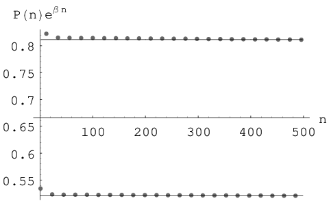
Expression (56) for the EFP fits the numerical data remarkably well (see Fig. 5) and this fact strongly supports the generalized Fisher-Hartwig conjecture.

One can understand these oscillations as a result of “superconducting” correlations of real fermions described by the Hamiltonian (7). Fermions are created and destroyed in pairs of nearest neighbors. At large magnetic fields, the oscillations are due to the fact that the probability of having a depletion string of length $2k-1$ or $2k$ is very similar. Since the magnetic field in (7) is essentially a chemical potential for the fermions, the energy cost to destroy a pair of particles is $4h$ : at very big magnetic fields, the amplitude for a pair destruction event is suppressed by a factor of $\gamma\over 4h$ , i.e. a probability of $\gamma^{2}\over 16h^{2}$ . This means that the probability of depletion behaves like:

	$\displaystyle P(2k-1)$	$\displaystyle\sim$	$\displaystyle 2\left({4h\over\gamma}\right)^{-2k}\qquad{\rm and}$
	$\displaystyle P(2k)$	$\displaystyle\sim$	$\displaystyle\left({4h\over\gamma}\right)^{-2k}\;,$		(59)

where the factor of two in the first expression is a simple combinatorial factor. The two probabilities in (59) can be combined in a single expression:

P(n)=E\left[1+A\cos(\pi n)\right]\left({4h\over\gamma}\right)^{-n},

(60)

which is precisely (56), with

A=1-{\gamma\over h}+{\rm O}\left({1\over h^{2}}\right).

(61)

We can check the correctness of this interpretation by taking the limit of (56) for $h>>1,\gamma$ . From (25) and (58) it is easy to find

	$\displaystyle\beta(h\to\infty,\gamma)$	$\displaystyle=$	$\displaystyle\log{4h\over\gamma}+\;{\rm O}\left({1\over h^{2}}\right)$		(62)
	$\displaystyle A_{+}(h\to\infty,\gamma)$	$\displaystyle=$	$\displaystyle 1-{\gamma\over h}+{\rm O}\left({1\over h^{2}}\right)$		(63)

in agreement with (60,61).

V.2 The critical lines ( $\Omega_{\pm}$ )

V.2.1 $\Omega_{+}$ ( $h=1$ )

For $h=1$ the generating function $\sigma(q)$ vanishes at $q=\pi$ and its phase has $\pi$ jumps at $q=0,\pi$ (see Fig. 2d). As in the previous section, the existence of two singular points gives rise to many terms of the form (107). However, in contrast to the $\Sigma_{+}$ region, the application of gFH as in (108) shows that all terms are suppressed by power law factors of $n$ with respect to the leading one.

The leading term is generated by the parametrization:

\sigma(q)=\tau^{1}(q){\rm e}^{{{\rm i}\over 2}[(q-\pi){\rm\>mod\>}2\pi-\pi]}\left(2-2\cos(q-\pi)\right)^{1/2}{\rm e}^{-{{\rm i}\over 4}[q{\rm\>mod\>}2\pi-\pi]}

(64)

and consists of an exponential decay with $\beta(1,\gamma)$ from (39) and a power law contribution with critical exponent $\lambda={1\over 16}$

\left|\det({\bf S_{n}})\right|\sim{\it E^{1}_{1}}(\gamma)n^{-{1\over 16}}\>{\rm e}^{-\beta(1,\gamma)n}

(65)

with

{\it E^{1}_{1}}(\gamma)\equiv E[\tau]G\left({3\over 4}\right)G\left({5\over 4}\right){\tau_{-}^{1/4}(0)\over 2^{1/4}\tau_{+}^{1/4}(0)\tau_{-}(\pi)},

(66)

where $G$ is the Barnes G-function defined in (104) and $E[\tau]$ is defined as in (48) with

\hat{\tau}_{k}=\hat{\sigma}_{k}+\left({1\over 4}-(-1)^{k}\right){1\over k}\;\theta(k)-{1\over 4k}\;\theta(-k),

(67)

with $\hat{\sigma}_{k}$ from (44).

The next term (subleading at $n\to\infty$ ) is obtained from the parametrization

\sigma(q)=\tau^{2}(q){\rm e}^{-{{\rm i}\over 2}[(q-\pi){\rm\>mod\>}2\pi-\pi]}\left(2-2\cos(q-\pi)\right)^{1/2}{\rm e}^{{\rm i}{3\over 4}[q{\rm\>mod\>}2\pi-\pi]}

(68)

and is given by

{\it E^{2}_{1}}(\gamma)(-1)^{n}n^{-{9\over 16}}\>{\rm e}^{-\beta(1,\gamma)n}

(69)

with

{\it E^{2}_{1}}(\gamma)\equiv E[\tau]G\left({1\over 4}\right)G\left({7\over 4}\right){\tau_{+}^{3/4}(0)\over 2^{3/4}\tau_{-}^{3/4}(0)\tau_{+}(\pi)}.

(70)

Although the inclusion of the latter (subleading) term is somewhat beyond even gFH, we write the sum of these two terms as a conjecture for EFP at $h=1$

P(n)\sim{\it E^{1}_{1}}(\gamma)\>n^{-{1\over 16}}\left[1+(-1)^{n}A_{1}(\gamma)/n^{1\over 2}\right]\>{\rm e}^{-\beta(1,\gamma)n}.

(71)

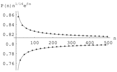
As these results rely on our unproven conjecture, we present our numerical data for this case in Fig. 6. Indeed, we see that the form (71) is in good agreement with numerics and this supports our hypothesis.

The amplitude of the oscillations is

$\displaystyle A_{1}(\gamma)$	$\displaystyle\equiv$	$\displaystyle{1\over\sqrt{2}}\;{G\left({1\over 4}\right)G\left({7\over 4}\right)\over G\left({3\over 4}\right)G\left({5\over 4}\right)}\;{\tau_{+}(0)\tau_{-}(\pi)\over\tau_{-}(0)\tau_{+}(\pi)}$	(72)
	$\displaystyle=$	$\displaystyle{1\over\sqrt{2}}\;{\Gamma\left({3\over 4}\right)\over\Gamma\left({1\over 4}\right)}\;{\tau(0)\over\tau(\pi)}\left({\tau_{-}(\pi)\over\tau_{-}(0)}\right)^{2}$
	$\displaystyle=$	$\displaystyle{\Gamma\left({3\over 4}\right)\over\Gamma\left({1\over 4}\right)}\;{1\over\gamma}\;\exp\left(4\lim_{\epsilon\rightarrow 0}\oint{{\displaystyle\rm\mathstrut d}z\over 2\pi}{\log\tau(z)\over z^{2}-(1+\epsilon)^{2}}\right),$

where we used (103) and the identity

G(z+1)=\Gamma(z)G(z).

(73)

To calculate the integral we deform the contour of integration as in Fig. 4e and find

A_{1}(\gamma)={\Gamma\left({3\over 4}\right)\over\Gamma\left({1\over 4}\right)}\;{1\over\sqrt{2\gamma}}.

(74)

We conclude that at $h=1$ the EFP decays exponentially at $n\to\infty$ but with an additional power law pre-factor and a damped oscillatory component.

Remark. It is curious to notice that the exponents $1/16$ and $9/16$ in (65) and (69) remind us of the scaling dimensions of spins $\sigma^{x}$ and $\sigma^{y}$ . ³³ 3 See Ref. mccoy, where it was shown that the power laws for the $\sigma^{x}$ and $\sigma^{y}$ correlators are $1/4$ and $9/4$ respectively. It looks as if the EFP operator (3), among other things, has inserted square roots of spins transverse to the magnetic field at the ends of the string.

V.2.2 $\Omega_{-}$ ( $h=-1$ )

For $h=-1$ the generating function $\sigma(q)$ does not vanish but has a phase discontinuity of $\pi$ at $q=\pi$ . We parametrize $\sigma(q)$ as

\sigma(q)=\tau^{1}(q){\rm e}^{-{{\rm i}\over 4}[(q-\pi){\rm\>mod\>}2\pi-\pi]}

(75)

and apply FH to obtain

P(n)\sim{\it E^{1}_{-1}(\gamma)}\>n^{-{1\over 16}}\>{\rm e}^{-\beta(-1,\gamma)n}

(76)

with

{\it E^{1}_{-1}}(\gamma)\equiv E[\tau]G\left({3\over 4}\right)G\left({5\over 4}\right){\tau_{-}^{1/4}(\pi)\over\tau_{+}^{1/4}(\pi))},

(77)

where $\beta(-1,\gamma)$ and $E[\tau]$ are defined in (40) and (48) with

\hat{\tau}_{k}=\hat{\sigma}_{k}+{(-1)^{k}\over 4k}\;\theta(k)-{(-1)^{k}\over 4k}\;\theta(-k)

(78)

and $\hat{\sigma}_{k}$ from (44).

We can stretch the gFH the same way as in the previous section for $h=+1$ by considering the second parametrization

\sigma(q)=\tau^{2}(q){\rm e}^{{\rm i}{3\over 4}[(q-\pi){\rm\>mod\>}2\pi-\pi]}

(79)

which gives

P^{\prime}(n)\sim{\it E^{2}_{-1}(\gamma)}\>n^{-{9\over 16}}\>{\rm e}^{-\beta(-1,\gamma)n}

(80)

with

{\it E^{2}_{-1}}(\gamma)\equiv E[\tau]G\left({1\over 4}\right)G\left({7\over 4}\right){\tau_{+}^{3/4}(\pi)\over\tau_{-}^{3/4}(\pi))}.

(81)

Adding this subleading term to (76) we obtain

P(n)\sim{\it E^{1}_{-1}}(\gamma)\>n^{-{1\over 16}}\left[1+A_{-1}(\gamma)/n^{1\over 2}\right]\>{\rm e}^{-n\beta(-1,\gamma)}

(82)

with

	$\displaystyle A_{-1}(\gamma)$	$\displaystyle\equiv$	$\displaystyle{G\left({1\over 4}\right)G\left({7\over 4}\right)\over G\left({3\over 4}\right)G\left({5\over 4}\right)}\;{\tau_{+}(\pi)\over\tau_{-}(\pi)}$		(83)
		$\displaystyle=$	$\displaystyle{\Gamma\left({3\over 4}\right)\over\Gamma\left({1\over 4}\right)}\;{\tau_{+}(\pi)\over\tau_{-}(\pi)}.$		(83)

We propose (82) as an asymptotic form for EFP at $h=-1$ .

VI The line $\Gamma_{E}$ : an exact calculation

Before we conclude our analysis of the EFP with the study of the isotropic XY model, let us check our results (42,25) on the special line⁴⁴ 4 We are grateful to Fabian Essler who suggested us to check our results on this special line and pointed out the reference shrock to us. in the phase diagram defined by

h^{2}+\gamma^{2}=1.

(84)

It was shown in Ref. shrock that on this line the ground state is a product of single spin states and is given by

|G\rangle=\prod_{j}|\theta,j\rangle=\prod_{j}\left[\cos\left({\theta\over 2}\right)|\uparrow,j\rangle+(-1)^{j}\sin\left({\theta\over 2}\right)|\downarrow,j\rangle\right],

(85)

where $|\uparrow,j\rangle$ is an up-spin state at the lattice site $j$ , etc. One can directly check that the state (85) is an eigenstate of (4) if the value of parameter $\theta$ is

\cos^{2}\theta=\frac{1-\gamma}{1+\gamma}

(86)

and (84) is satisfied. It is also easy to show shrock that this state is, in fact, the ground state of (4).

The probability of formation of a ferromagnetic string in the state (85) is obviously

P(n)=\sin^{2n}\left({\theta\over 2}\right)=\left({1\over 2}-{1\over 2}{h\over|h|}\sqrt{1-\gamma\over{1+\gamma}}\right)^{n},

(87)

which is an exact result on the line (84). The value of $\beta(h,\gamma)$ which immediately follows from this exact result is

\beta(h=\pm\sqrt{1-\gamma^{2}},\gamma)=-\log\left({1\over 2}\mp{1\over 2}\sqrt{1-\gamma\over{1+\gamma}}\right)=-\Lambda(h,\gamma),

(88)

where $\Lambda(h,\gamma)$ was defined in (32).

This is, indeed, consistent with (36) since under the condition (84) the function $\Delta(h,\gamma)$ vanishes. The integral (33) defining $\Delta(h,\gamma)$ vanishes for (84) because the branching points (29) and (30) collapse to the same point and therefore the region of integration shrinks to just one point (33). In fact, the Toeplitz matrix (21) generated by (22) becomes triangular on the line (84) with diagonal matrix element $(S_{n})_{jj}=\sin^{2}(\theta/2)$ and the determinant of ${\bf S_{n}}$ is exactly (87).

From the definitions of $\beta(h,\gamma)$ , we see that the decay factor consists of two terms, which have now a clear physical meaning. The $\Lambda(h,\gamma)$ term is the factor we found above in (88) and represents the contribution given by un-entangled spins. The remaining part accounts for the correlations between spins. Both $\Delta(h,\gamma)$ and the correlation functions given by (12) and (13) vanish on the line (84).

VII The critical line $\Omega_{0}$ ( $\gamma=0$ ) and the Gaussian behavior

The case $\gamma=0$ , corresponding to the Isotropic XY Model, has been studied in Ref. shiroishi. For $\gamma=0$ the generating function (22) is reduced to the one found in shiroishi.

For $|h|<1$ , the generating function $\sigma(q)$ has a limited support between $[-\cos^{-1}h,\cos^{-1}h]$ . To find the asymptotic behavior of the determinant of the Toeplitz matrix one can apply Widom’s Theorem widomsupp and obtain shiroishi

P(n)\sim 2^{5\over 24}{\rm e}^{3\zeta^{\prime}(-1)}(1-h)^{-{1\over 8}}n^{-{1\over 4}}\left({1+h\over 2}\right)^{n^{2}\over 2}.

(89)

We see that in this case, the EFP decays as a Gaussian with an additional power-law pre-factor.

In a different context, the formula (89) appeared also in dysmehta as a probability of forming a gap in the spectrum of unitary random matrices. This is not unexpected, since the joint eigenvalue distribution of unitary random matrices is known to coincide with the distribution of free fermions in the ground state.

For $|h|>1$ , the theory is no longer critical and the ground state is completely polarized in the $z$ direction, giving a trivial EFP $P(n)=0$ for $h>1$ and $P(n)=1$ for $h<-1$ .

VIII Crossover between Gaussian and exponential behavior: a Bosonization approach

In order to understand qualitatively the crossover between the Gaussian asymptotic behavior at $\gamma=0$ and the exponential decay for $\gamma\neq 0$ , we employ a bosonization approach similar to the one used in abanovkor. In the limit $\gamma\ll 1$ we consider the continuum limit of (8), bosonize the fermionic fields, and write the Euclidean action of the theory as ${\cal S}=\int{\displaystyle\rm\mathstrut d}x\,{\displaystyle\rm\mathstrut d}\tau{\cal L}$ , where $\tau\equiv{\rm i}t$ is the imaginary time and the Lagrangian is

{\cal L}=2\sin k_{F}\left[\left(\partial_{\mu}\vartheta\right)^{2}-{\gamma\over\pi}\cos\left(\sqrt{4\pi}\vartheta\right)\right].

(90)

Here $k_{F}=\cos^{-1}h$ is the Fermi momentum at $\gamma=0$ .

This is a Sine-Gordon theory for the “conjugate field” $\vartheta(x,\tau)$ , which describes the imaginary time dynamics of our 1-D system. In terms of $\vartheta$ the density of fermions is given by $\rho=\partial_{\tau}\vartheta+\rho_{0}$ , where $\rho_{0}=k_{F}/\pi$ is the density of fermions in the ground state.

In the field theory approach, the EFP (see Ref. abanovkor) in the limit $n\to\infty$ would be given with exponential accuracy by the probability of an instanton $P(n)\sim e^{-{\cal S}_{0}}$ , where ${\cal S}_{0}$ is the action of the instanton. Here the instanton is the solution of the classical equations of motion of (90) which corresponds to the formation of an emptiness of length $n$ at the time $\tau=0$ . Unfortunately, the EFP instanton involves large deviations of the density of fermions from the equilibrium density $\rho_{0}$ and is beyond the bosonization approach as the derivation of (90) relies on the linearization of the fermionic spectrum near the Fermi points.

Following abanovkor, we are going to slightly generalize our problem, by considering the depletion formation probability instead of the EFP requiring

\left.\rho\right|_{t=0,\;0<x<n}=\rho_{0}+\left.\partial_{t}\vartheta(x,t)\right|_{t=0,\;0<x<n}=\rho_{0}-\bar{\rho},

(91)

where $\bar{\rho}$ is some constant. The original EFP problem corresponds to $\bar{\rho}=\rho_{0}$ . Here, instead, we consider the probability of weak depletion, i.e.

-\left.\partial_{t}\vartheta(x,t)\right|_{t=0,\;0<x<n}=\bar{\rho}<<\rho_{0}.

(92)

We study the latter using an instanton approach to (90) and infer the (qualitative) behavior of the original EFP from this weak limit.

To simplify the problem further, we assume that the instanton configuration is completely confined to one of the wells of the Cosine potential in (90) and that the field $\vartheta$ is small enough to allow for an expansion of the Cosine:

{\cal S}\approx 2\sin k_{F}\int{\displaystyle\rm\mathstrut d}x\;{\displaystyle\rm\mathstrut d}\tau\left[\left(\partial_{\mu}\vartheta\right)^{2}+2\gamma\;\vartheta^{2}\right].

(93)

In this formulation, the anisotropy parameter $\gamma^{1/2}$ plays the role of the mass of the bosonized theory. The probability we are looking for is given by the action ${\cal S}_{0}$ of the classical field configuration which satisfies the Euler-Lagrange equation (in this case a Klein-Gordon equation in two dimensions) with the boundary condition (91)

P_{\bar{\rho}}(n)={\rm e}^{-{\cal S}_{0}}.

(94)

In the limit $\gamma=0$ , the theory is massless and scale invariant. In abanovkor it was shown that, due to the scale invariance, the action of the instanton is quadratic in $n$ . The instanton configuration in this case is essentially a droplet of depletion in space-time with dimensions proportional to $n$ both in the space and time direction, in order to satisfy the boundary condition (91). This result is consistent with the Gaussian asymptotic behavior prescribed by Widom’s theorem (see Sec. VII).

In the massive case, a finite correlation length $\xi\sim\gamma^{-1/2}$ is generated and one has a crossover behavior. For string lengths $n$ smaller than the correlation length $\gamma^{-1/2}$ , the instanton action is not sensitive to the presence of the finite correlation length and is still quadratic in $n$ (giving a Gaussian decay for EFP). In the asymptotic limit of string lengths greater than $\gamma^{-1/2}$ , the time dimension of a depletion droplet is of the order of $\xi$ (instead of $n$ as in the massless limit): the action is linear in $n$ and the probability has an exponential behavior.⁵⁵ 5 This picture is very similar to the one for massless theory at finite temperature. In the latter the inverse temperature plays the role of the correlation length abanovkor (see C).

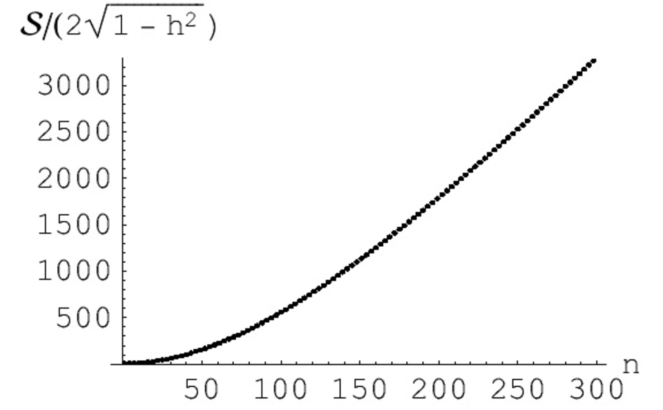
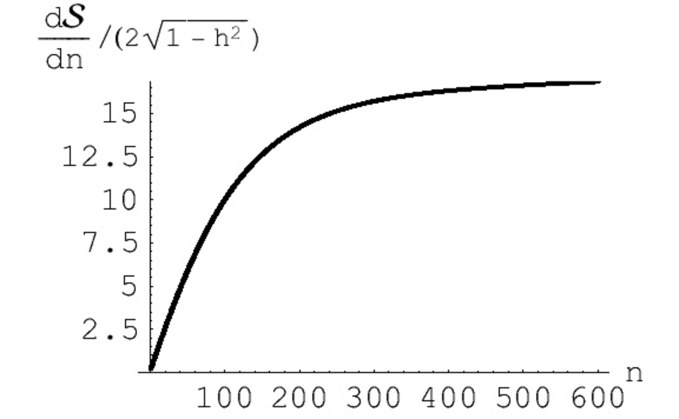
In Appendix C we show how to solve the integral equation corresponding to the boundary problem (91,93) and present its numerical solution and some analytical results. Figures 8 and 8 clearly show the crossover between a quadratic behavior of the stationary action for small $n$ to a linear asymptotic one for $n\to\infty$ .

IX Discussion and Conclusions

The asymptotic behavior of the Emptiness Formation Probability $P(n)$ as $n\to\infty$ for the Anisotropic XY model in a transverse magnetic field as a function of the anisotropy $\gamma$ and the magnetic field $h$ has been studied. We have summarized our results in Table 1. These asymptotic behaviors have already been presented in abanovfran. In this work, we completed the derivations by providing explicit expressions for the coefficients of these asymptotic forms.

Our main motivation has been to study the relation between the criticality of the theory and the asymptotics of the EFP. Let us now consider the results on the critical lines ( $\Omega_{0}$ and $\Omega_{\pm}$ ). The Gaussian behavior on $\Omega_{0}$ ( $\gamma=0$ , $|h|<1$ ) is in accord with the qualitative argument of Ref. abanovkor using a field theory approach. In $\Sigma_{0}$ ( $\gamma\neq 0$ , $|h|<1$ ) the asymptotic decay is exponential. We proposed a physical interpretation of the crossover between the two asymptotes using a bosonization analysis of the region of small $\gamma$ : we suggest that there is an intermediate regime of Gaussian decay for the string lengths smaller than $1/\sqrt{\gamma}$ which crosses over to the exponential behavior for longer strings.

On the critical lines $\Omega_{\pm}$ , the decay of the EFP is exponential instead of Gaussian, and apparently contradicts the qualitative picture of Ref. abanovkor. The reason for this disagreement is that although at $h=\pm 1$ the model can be rewritten in terms of massless quasiparticles $\chi$ defined in (9), we are still interested in the EFP for the “original” Jordan-Wigner fermions $\psi$ . In terms of $\chi$ this correlator has a complicated (nonlocal) expression very much different from the simple one (14). From the technical point of view, the difference is that in the qualitative argument in favor of a Gaussian decay of EFP for critical systems there is an implicit assumption that the density of fermions (or magnetization) is related in a local way to the field responsible for the critical degrees of freedom (free boson field $\phi$ ). This assumption is not valid on the lines $h=\pm 1$ . The theory is critical on those lines and can be described by some free field $\phi$ . However, the relation between the magnetization and this field is highly nonlocal and one can not apply the simple argument of abanovkor to the XY model at $h=\pm 1$ .

Although EFP at the critical magnetic field does not show a Gaussian behavior, there is an important difference between the asymptotic behavior of EFP on and off critical lines. Namely, a power-law pre-factor $n^{-\lambda}$ appears on all critical lines. For the XY model it is universal (i.e. $\lambda$ is constant on a given critical line) and takes values $\lambda=1/4$ for $\gamma=0$ shiroishi and $\lambda=1/16$ on the lines $h=\pm 1$ . It would be interesting to understand which operators determine these particular “scaling dimensions” of the EFP (see the remark at the end of Section V.2.1).

At $h\geq 1$ the use of gFH predicts even-odd oscillations of $P(n)$ . We compared the predicted oscillations to numerical calculations of Toeplitz determinants and found a very good agreement (see Figs. 5,6). We proposed a physical interpretation of the oscillations as coming from pair correlations of spins which can be clearly seen as superconducting correlations in the fermionic representation (7).

In some parts of the phase diagram ( $\Sigma_{+}$ , $\Omega_{\pm}$ ) we used the so-called generalized Fisher-Hartwig conjecture basor which is not yet proven. However, our numeric calculations support the analytical results (see Figures 5 and 6). We note that to the best of our knowledge this is the first physically motivated example where the original Fisher-Hartwig conjecture fails and its extended version is necessary. ⁶⁶ 6 We note that recently the theory on Toeplitz determinants has been used and extended with new results in order to calculate yet one more important physical quantity. We refer the interested reader to korepin03, korepin04 and keating, where the entaglement for the XY Spin chain and for Random matrix models have been calculated. We also suggest that the gFH could be used to find the subleading corrections to the asymptotic behavior, as we did for $h=\pm 1$ in (71,82). This novel hypothesis is supported by our numerics and it would be interesting to confirm it analytically.

In conclusion, we notice that it is straightforward to generalize our results for nonzero temperature. The only modification is that at $T\neq 0$ the thermal correlation functions must be used instead of (12,13). Then, the generating function (22) is non-singular everywhere and we have an exponential decay of $P(n)$ in the whole phase diagram according to the standard Szegö Theorem and standard statistical mechanics arguments. We present results for $T\neq 0$ in Appendix B.

X Acknowledgments

We greatly benefited from multiple discussions with F. Essler, V.E. Korepin, and B.M. McCoy. The work of AGA was supported by the NSF grant DMR-0348358, and the Theory Institute of Strongly Correlated and Complex Systems at Brookhaven.

Appendix A Asymptotic behavior of Toeplitz Determinants

The asymptotic behavior of the EFP for (4) at $n\to\infty$ is exactly related to the asymptotic behavior of the determinant of the corresponding Toeplitz matrix (21,22,23) and can be extracted from known theorems and conjectures in the theory of Toeplitz matrices. These types of calculations have been done first in LSM-1961; mccoy for spin-spin correlation functions. It is well known that the asymptotic behavior of the determinant of a Toeplitz matrix as the size of the matrix goes to infinity strongly depends upon the zeros and singularities of the generating function of the matrix.

A very good report on the subject has been recently compiled by T. Ehrhardt Ehrhardt-2001. Here we want to recap what is known about the determinant of a Toeplitz matrix generated by a function $\sigma(q)$ :

D_{n}[\sigma]=\det({\bf S_{n}})=\det\left(\int_{-\pi}^{\pi}\sigma(q){\rm e}^{-{\rm i}(j-k)q}{{\displaystyle\rm\mathstrut d}q\over 2\pi}\right)_{j,k=0}^{n},

(95)

where the generating function $\sigma(q)$ is a periodic (complex) function, i.e. $\sigma(q)=\sigma(2\pi+q)$ . In this work we dealt only with generating functions with zero winding number

{\rm Ind}\,\sigma(q)\equiv\int_{-\pi}^{\pi}{{\displaystyle\rm\mathstrut d}q\over 2\pi}\,{{\displaystyle\rm\mathstrut d}\over{\displaystyle\rm\mathstrut d}q}\log\sigma(q)=0

(96)

and this brief review will be limited to this condition. This was not the case in the study of Barouch et al. mccoy, where the generating function (see footnote after (23)) had non-zero winding number in some regions of the phase diagram.

A.1 The Strong Szegö Theorem

If $\sigma(q)$ is sufficiently smooth, non-zero and satisfies ${\rm Ind}\,\sigma(q)=0$ (i.e., the winding number is $0$ ), we can apply what is known as the Strong Szegö Limit Theorem (Hirschman, mccoywu), which states that the determinant has a simple exponential asymptotic form

D_{n}[\sigma]\sim E[\sigma]G[\sigma]^{n}\qquad n\rightarrow\infty,

(97)

where $G[\sigma]$ and $E[\sigma]$ are defined by

G[\sigma]\equiv\exp{\hat{\sigma}_{0}},\qquad E[\sigma]\equiv\exp{\sum_{k=1}^{\infty}k\hat{\sigma}_{k}\hat{\sigma}_{-k}}

(98)

and $\hat{\sigma}_{k}$ are the Fourier coefficients of the expansion of the logarithm of $\sigma(q)$ :

\log\sigma(q)\equiv\sum_{k=-\infty}^{\infty}\hat{\sigma}_{k}{\rm e}^{{\rm i}kq}.

(99)

A.2 The Fisher-Hartwig Conjecture

Over the years, the Szegö Theorem has been extended to consider broader classes of generating functions by relaxing the continuity conditions which define a ”smooth function”, but it remained limited to never-vanishing functions. Therefore, some extensions have been proposed to the Szegö Theorem in order to relax this latter hypothesis. When the generating function has only pointwise singularities (or zeros), there exists a conjecture known as the Fisher-Hartwig Conjecture (FH) FisherHartwig-1968. ⁷⁷ 7 This conjecture is still not completely proven. For details and status of the conjecture see Ref. basor.

When $\sigma(q)$ has $R$ singularities at $q=\theta_{r}$ ( $r=1..R$ ), we decompose it as follows:

\sigma(q)=\tau(q)\prod_{r=1}^{R}{\rm e}^{{\rm i}\kappa_{r}[(q-\theta_{r}){\rm\>mod\>}2\pi-\pi]}\left(2-2\cos(q-\theta_{r})\right)^{\lambda_{r}}

(100)

so that $\tau(q)$ is a smooth function satisfying the conditions stated in the previous section. Then according to FH the asymptotic formula for the determinant takes the form

D_{n}[\sigma]\sim E\left[\tau,\{\kappa_{a}\},\{\lambda_{a}\},\{\theta_{a}\}\right]\;n^{\sum_{r}\left(\lambda_{r}^{2}-\kappa_{r}^{2}\right)}G[\tau]^{n}\qquad n\rightarrow\infty,

(101)

where the constant prefactor is conjectured to be

$\displaystyle E\left[\tau,\{\kappa_{a}\},\{\lambda_{a}\},\{\theta_{a}\}\right]\equiv$	$\displaystyle E[\tau]$	$\displaystyle\prod_{r=1}^{R}\tau_{-}\left({\rm e}^{{\rm i}\theta_{r}}\right)^{-\kappa_{r}-\lambda_{r}}\tau_{+}\left({\rm e}^{-{\rm i}\theta_{r}}\right)^{\kappa_{r}-\lambda_{r}}$	(102)
	$\displaystyle\times$	$\displaystyle\prod_{1\leq r\neq s\leq R}\left(1-{\rm e}^{{\rm i}(\theta_{s}-\theta_{r})}\right)^{(\kappa_{r}+\lambda_{r})(\kappa_{s}-\lambda_{s})}$
	$\displaystyle\times$	$\displaystyle\prod_{r=1}^{R}{{\rm G}(1+\kappa_{r}+\lambda_{r}){\rm G}(1-\kappa_{r}+\lambda_{r})\over{\rm G}(1+2\lambda_{r})}.$

$E[\tau]$ and $G[\tau]$ are defined as in (98) and $\tau_{\pm}$ are defined by decomposition

\tau(q)=\tau_{-}\left({\rm e}^{{\rm i}q}\right)G[\tau]\tau_{+}\left({\rm e}^{-{\rm i}q}\right),

(103)

so that $\tau_{+}$ ( $\tau_{-}$ ) are analytic and non-zero inside (outside) the unit circle on which $\tau$ is defined and satisfy the boundary conditions $\tau_{+}(0)=\tau_{-}(\infty)=1$ . ${\rm G}$ is the Barnes G-function, an analytic entire function defined as

{\rm G}(z+1)\equiv(2\pi)^{z/2}{\rm e}^{-[z+(\gamma_{E}+1)z^{2}]/2}\prod_{n=1}^{\infty}\left(1+{z\over n}\right)^{k}{\rm e}^{-z+{z^{2}\over 2n}},

(104)

where $\gamma_{E}\sim 0.57721\ldots$ is the Euler-Mascheroni Constant.

This conjecture is actually proven for some ranges of parameters $\kappa_{r}$ and $\lambda_{r}$ or fully for the case of a single singularity ( $R=1$ ), see widomsing; Ehrhardt-1997.

In many simple cases it is possible to find the factorization of $\tau$ into the product of $\tau_{+}$ and $\tau_{-}$ by inspection. More complicated examples like the ones presented in this work require a special technique to obtain this factorization, which is known as the Wiener-Hopf decomposition:

	$\displaystyle\log\tau_{+}(w)=\oint{{\displaystyle\rm\mathstrut d}z\over 2\pi{\rm i}}{\log\tau(z)\over z-w}$		$\displaystyle\|w\|<1,$
	$\displaystyle\log\tau_{-}(w)=-\oint{{\displaystyle\rm\mathstrut d}z\over 2\pi{\rm i}}{\log\tau(z)\over z-w}$		$\displaystyle\|w\|>1,$		(105)

where the integral is taken over the unit circle.

In light of these formulas, it is useful to present the parametrization (100) in a form which makes the analytical structure more apparent. Changing the variable dependence from $q$ to $z\equiv{\rm e}^{{\rm i}q}$ , we write

\sigma(z)=\tau(z)\prod_{r=1}^{R}\left(1-{z\over z_{r}}\right)^{\lambda_{r}+\kappa_{r}}\left(1-{z_{r}\over z}\right)^{\lambda_{r}-\kappa_{r}},

(106)

where $z_{r}\equiv{\rm e}^{{\rm i}\theta_{r}}$ .

A.3 The Generalized Fisher-Hartwig Conjecture

Despite the considerable success of the Fisher-Hartwig Conjecture, few examples have been reported in the mathematical literature that do not fit this result. These examples share the characteristics that inequivalent representations of the form (100) exist for the generating function $\sigma(q)$ . Although no theorem has been proven concerning these cases, a generalization of the Fisher-Hartwig Conjecture (gFH) has been suggested by Basor and Tracy basor that has no counter-examples yet.

If more than one parametrization of the kind (100) exists, we write them all as

\sigma(q)=\tau^{i}(q)\prod_{r=1}^{R}{\rm e}^{{\rm i}\kappa^{i}_{r}[(q-\theta_{r}){\rm\>mod\>}2\pi-\pi]}\left(2-2\cos(q-\theta_{r})\right)^{\lambda^{i}_{r}},

(107)

where the index $i$ labels different parametrizations (for $R>1$ there can be only a countable number of different parametrizations of this kind). Then the asymptotic formula for the determinant is

D_{n}[\sigma]\sim\sum_{i\in\Upsilon}E\left[\tau^{i},\{\kappa^{i}_{a}\},\{\lambda^{i}_{a}\},\{\theta_{a}\}\right]\;n^{\Omega(i)}G[\tau^{i}]^{n}\qquad n\rightarrow\infty,

(108)

where

	$\displaystyle\Omega(i)$	$\displaystyle\equiv$	$\displaystyle\sum_{r=1}^{R}\left(\left(\lambda^{i}_{r}\right)^{2}-\left(\kappa^{i}_{r}\right)^{2}\right),$		(109)
	$\displaystyle\Upsilon$	$\displaystyle=$	$\displaystyle\left\{i\>\\|\>\mbox{Re}\,[\Omega(i)]=\max_{j}\mbox{Re}\,[\Omega(j)]\right\}.$		(110)

The generalization essentially gives the asymptotics of the Toeplitz determinant as a sum of (FH) asymptotics calculated separately for different leading (see Eq. (110)) representations (107). In Sec. V.2.1 we used the sum of all (not necessarily leading) representations and showed that it also correctly produces the first subleading corrections to the asymptotics of our Toeplitz determinant.

A.4 Widom’s Theorem

If $\sigma(q)$ is supported only in the interval $\alpha\leq q\leq 2\pi-\alpha$ as in our model for $\gamma=0$ , singularities are no longer pointwise and one should apply Widom’s Theorem widomsupp. It states that the asymptotic behavior of the determinant in this case is

D_{n}[\sigma]\sim 2^{1/12}{\rm e}^{3\zeta^{\prime}(-1)}\left(\sin{\alpha\over 2}\right)^{-1/4}E[\rho]^{2}n^{-1/4}G[\rho]^{n}\left(\cos{\alpha\over 2}\right)^{n^{2}},

(111)

where $E$ and $G$ are defined in (98) and

\rho(q)=\sigma\left(2\cos^{-1}\left[\cos{\alpha\over 2}\cos q\right]\right)

(112)

with the convention $0\leq\cos^{-1}x\leq\pi$ .

For the case considered in Section VII, the generating function is constant, $E[\rho]=G[\rho]=1$ , and (111) simplifies considerably giving

D_{n}[\sigma]\sim 2^{1/12}{\rm e}^{3\zeta^{\prime}(-1)}\left(\sin{\alpha\over 2}\right)^{-1/4}n^{-1/4}\left(\cos{\alpha\over 2}\right)^{n^{2}}.

(113)

Appendix B Emptiness Formation Probability at finite temperature

At finite temperature ( $T>0$ ), the correlators (12) and (13) become

	$\displaystyle F_{jk}^{T}$	$\displaystyle\equiv$	$\displaystyle{\rm i}\langle\psi_{j}\psi_{k}\rangle_{T}=-{\rm i}\langle\psi_{j}^{\dagger}\psi_{k}^{\dagger}\rangle_{T}=\int_{0}^{2\pi}{{\displaystyle\rm\mathstrut d}q\over 2\pi}{1\over 2}\sin\vartheta_{q}\tanh{\varepsilon_{q}\over 2T}{\rm e}^{{\rm i}q(j-k)},$		(114)
	$\displaystyle G_{jk}^{T}$	$\displaystyle\equiv$	$\displaystyle\langle\psi_{j}\psi_{k}^{\dagger}\rangle_{T}=\int_{0}^{2\pi}{{\displaystyle\rm\mathstrut d}q\over 2\pi}{1\over 2}\left(1+\cos\vartheta_{q}\tanh{\varepsilon_{q}\over 2T}\right){\rm e}^{{\rm i}q(j-k)}.$		(115)

The EFP is expressed by (2) and in the spinless fermion formalism it becomes

P(n)=\langle\prod_{i=1}^{n}\psi_{i}\psi_{i}^{\dagger}\rangle_{T}.

(116)

We again use Wick’s Theorem (or its thermal version, called Bloch-de Dominicis theorem todakubo) to express it as a Pfaffian. The calculation proceeds the same way as for zero temperature and the EFP can be represented as

P(n)=|\det({\bf T_{n}})|,

(117)

where ${\bf T_{n}}$ is the $n\times n$ Toeplitz matrix generated by the function

t(q)={1\over 2}\left(1+{\rm e}^{{\rm i}\vartheta_{q}}\tanh{\varepsilon_{q}\over 2T}\right)

(118)

where the “rotation angle” $\vartheta_{q}$ and the spectrum $\varepsilon_{q}$ were defined in (10) and (11) respectively.

The generating function $t(q)$ is never-vanishing and has zero winding number. Therefore, for $T>0$ we can apply the standard Szegö Theorem to obtain

P(n){\stackrel{{\scriptstyle n\rightarrow\infty}}{{\sim}}}E(h,\gamma,T){\rm e}^{-n\beta(h,\gamma,T)},

(119)

where

$\displaystyle\beta(h,\gamma,T)$	$\displaystyle=$	$\displaystyle-\int_{0}^{2\pi}{{\displaystyle\rm\mathstrut d}q\over 2\pi}\;\log\left\|t(q)\right\|$	(120)
	$\displaystyle=$	$\displaystyle-{1\over 2}\int_{0}^{2\pi}{{\displaystyle\rm\mathstrut d}q\over 2\pi}\;\log\left[{1\over 2}\left(1+{\cos q-h\over\varepsilon_{q}}\tanh{\varepsilon_{q}\over 2T}\right)\right],$	(120)
$\displaystyle E(h,\gamma,T)$	$\displaystyle=$	$\displaystyle\exp\left(\sum_{k=1}^{\infty}k\hat{t}_{k}\hat{t}_{-k}\right)$	(121)

with

\hat{t}_{k}=\int_{0}^{2\pi}{{\displaystyle\rm\mathstrut d}q\over 2\pi}{\rm e}^{-{\rm i}kq}\log\left[{1\over 2}\left(1+{\cos q-h+{\rm i}\gamma\sin q\over\varepsilon_{q}}\tanh{\varepsilon_{q}\over 2T}\right)\right],

(122)

and $\varepsilon_{q}$ is given as in (11) by

\varepsilon_{q}=\sqrt{(\cos q-h)^{2}+\gamma^{2}\sin^{2}q}.

(123)

As can be expected from simple thermodynamic considerations, at finite temperature the behavior is always purely exponential asymptotically. As it was shown in abanovkor, at finite but very low temperatures one can observe a crossover from the zero temperature behavior at short string lengths $n$ to the exponential behavior (119) in the limit of very large $n$ . This crossover occurs at a length scale of the order of the inverse temperature.

Appendix C Calculation of the stationary action in the bosonization approach

In Section VIII we have formulated the XY model near $\gamma=0$ in terms of the bosonic field with Lagrangian (93). It was also pointed out that, instead of the EFP, we are interested in the Probability of Formation of Weakly Ferromagnetic Strings (PFWFS) and that we are going to calculate this probability in the saddle point approximation. Therefore, we consider a configuration of the field (instanton) which satisfies the boundary condition imposed by the PFWFS (91,92)

\left.\partial_{t}\vartheta(x,t)\right|_{t=0,0<x<n}=\bar{\rho}

(124)

and that minimizes the action, i.e. that satisfies the Euler-Lagrange equations:

\left(\partial_{\mu}\partial^{\mu}-m^{2}\right)\vartheta=0.

(125)

The latter equation is the Klein-Gordon equation with the mass given by $m^{2}\equiv 2\gamma$ (see (93)). The PFWFS will be found from the value of the action ${\cal S}_{0}$ corresponding to this instanton configuration (94). In this appendix we calculate the stationary action needed in Sec. VIII.

We now solve the differential equation (125) with non-trivial boundary condition (124) by recasting it as the integral equation:

\vartheta(x,t)={1\over 2\pi}\int_{0}^{n}\partial_{t}K_{0}\left(m\sqrt{(x-y)^{2}+t^{2}}\right)f(y)\;{\displaystyle\rm\mathstrut d}y,

(126)

where $K_{0}(x,x^{\prime};t,t^{\prime})$ is the modified Bessel function of 0-th order – the kernel of the differential operator (125) in two dimensions. We impose the boundary condition (124) by requiring that the “source” $f(y)$ satisfies

	$\displaystyle\left.\partial_{t}\vartheta(x,0)\right\|_{0<x<n}$	$\displaystyle=$	$\displaystyle\lim_{t\to 0}{1\over 2\pi}\int_{0}^{n}\left\{K_{2}\left(m\sqrt{(x-y)^{2}+t^{2}}\right){m^{2}t^{2}\over(x-y)^{2}+t^{2}}\right.$		(127)
			$\displaystyle\quad\left.-\,K_{1}\left(m\sqrt{(x-y)^{2}+t^{2}}\right){m\over\sqrt{(x-y)^{2}+t^{2}}}\right\}f(y)\;{\displaystyle\rm\mathstrut d}y=\bar{\rho}.$		(127)

This is the integral equation on $f(y)$ we have to solve.

Once the limit $t\to 0$ is taken, the kernel in Eq. (127) is singular. We isolate the singularity by rewriting equation (127) as:

{{\displaystyle\rm\mathstrut d}\over{\displaystyle\rm\mathstrut d}x}\;\mathchoice{{\vbox{\hbox{$\textstyle-$}}\kern-4.86108pt}}{{\vbox{\hbox{$\scriptstyle-$}}\kern-3.43057pt}}{{\vbox{\hbox{$\scriptscriptstyle-$}}\kern-2.908pt}}{{\vbox{\hbox{$\scriptscriptstyle-$}}\kern-2.76045pt}}\!\int_{0}^{n}{f(y)\over x-y}\;{\displaystyle\rm\mathstrut d}y+\lim_{t\to 0}\int_{0}^{n}G_{0}(x,t;y)f(y)\;{\displaystyle\rm\mathstrut d}y=2\pi\bar{\rho}

(128)

with

	$\displaystyle G_{0}(x,t;y)$	$\displaystyle\equiv$	$\displaystyle{(x-y)^{2}-t^{2}\over(x-y)^{2}+t^{2}}+K_{2}\left(m\sqrt{(x-y)^{2}+t^{2}}\right){m^{2}t^{2}\over(x-y)^{2}+t^{2}}$		(129)
			$\displaystyle-K_{1}\left(m\sqrt{(x-y)^{2}+t^{2}}\right){m\over\sqrt{(x-y)^{2}+t^{2}}}$		(129)

or, after integration over $x$ , as

\mathchoice{{\vbox{\hbox{$\textstyle-$}}\kern-4.86108pt}}{{\vbox{\hbox{$\scriptstyle-$}}\kern-3.43057pt}}{{\vbox{\hbox{$\scriptscriptstyle-$}}\kern-2.908pt}}{{\vbox{\hbox{$\scriptscriptstyle-$}}\kern-2.76045pt}}\!\int_{0}^{n}{f(y)\over x-y}\;{\displaystyle\rm\mathstrut d}y+\int_{0}^{n}G(x;y)f(y)\;{\displaystyle\rm\mathstrut d}y=2\pi\bar{\rho}\;x

(130)

with

G(x;y)\equiv\lim_{t\to 0}\int_{0}^{x}G_{0}(x_{1},t;y)\;{\displaystyle\rm\mathstrut d}x_{1}.

(131)

We have recasted Eq. (127) in the standard form for a singular integral equation (130). Once we have the solution of this equation, we can calculate the action corresponding to this instanton as

{\cal S}_{0}=4\sqrt{1-h^{2}}\bar{\rho}\int_{0}^{n}f(y)\;{\displaystyle\rm\mathstrut d}y.

(132)

We solved singular integral equation (130) numerically and we computed the corresponding action (132). The results of these calculation are presented as a plot of the action ${\cal S}_{0}$ vs. $n$ in Fig. 8, where we notice the crossover from a quadratic to a linear behavior (corresponding to a crossover from Gaussian to exponential behavior for the probability, (94)) as we expected. To confirm the nature of this crossover, in Fig. 8 we plot $d{\cal S}_{0}/dn$ and we see that it starts linearly and then saturates asymptotically as it should.

In the limit $n\ll 1/m$ , we can expand the Bessel functions in the kernel (129)

G_{0}(x,t;y)=-{m^{2}\over 2}\left({t^{2}\over(x-y)^{2}+t^{2}}+{1\over 2}\ln\left[(x-y)^{2}+t^{2}\right]+\ln{m\over 2}+G-{1\over 2}\right)+\ldots,

(133)

where $G$ is Catalan’s constant. Then we solve the singular integral equation (130) to first order by first transforming it into a regular integral equation.

In musk, Chap. 14, Sec. 114 it is explained that a singular integral equation like (130) is equivalent to

f(x)+{1\over\pi{\rm i}}\int_{0}^{n}N(x;y)\;f(y)\;{\displaystyle\rm\mathstrut d}y=2\bar{\rho}\sqrt{x(n-x)},

(134)

where the new kernel is

N(x;y)\equiv{\sqrt{x(n-x)}\over\pi{\rm i}}\;\mathchoice{{\vbox{\hbox{$\textstyle-$}}\kern-4.86108pt}}{{\vbox{\hbox{$\scriptstyle-$}}\kern-3.43057pt}}{{\vbox{\hbox{$\scriptscriptstyle-$}}\kern-2.908pt}}{{\vbox{\hbox{$\scriptscriptstyle-$}}\kern-2.76045pt}}\!\int_{0}^{n}{G(y^{\prime};y)\over\sqrt{y^{\prime}(n-y^{\prime})}(x-y^{\prime})}\;{\displaystyle\rm\mathstrut d}y^{\prime}.

(135)

Using (133), we can explicitly calculate the integral defining $N(x;y)$ in terms of elementary functions and after some algebra the integral equation (134) results in a long, but essentially simple, regular integral equation. Its solution is

f(x)=\bar{\rho}\left[2+{m^{2}n^{2}\over 8}\left(\ln{m\,n\over 8}+G-{3\over 2}\right)\right]\sqrt{x(n-x)}-\bar{\rho}\;{m^{2}n^{2}\over 4}\left(x-{n\over 2}\right)\tan^{-1}\sqrt{x\over n-x}.

(136)

The corresponding stationary action (132) is

{\cal S}_{0}=\pi\sqrt{1-h^{2}}\bar{\rho}^{2}n^{2}\left[1+{m^{2}n^{2}\over 16}\left(\ln{m\;n\over 8}+G-2\right)\right].

(137)

The first term in (137) corresponds to the Gaussian decay of PFWFS we expect in the limit of $m=0$ . In Fig. 9, we compare this analytical result for the action with the numerical result of Fig.8. In the plot, we include the pure Gaussian decay (the first term in (137)), which already gives a remarkable agreement for small $n$ . The full solution (137) extends this agreement further for larger $n$ .

References

(1) H. Bethe, Zeitschrift für Physik, 71, 205 (1931).
Zur Theorie der Metalle: I. Eingenwerte and Eigenfunktionen der linearen Atomkette.
(2) C.N. Yang, and C.P. Yang, Phys. Rev. 150, 327, (1966).
One-Dimensional Chain of Anisotropic Spin-Spin Interactions. II. Properties of the Ground-State Energy Per Lattice Site for an Infinite System.
(3) V.E. Korepin, N.M. Bogoliubov, and A.G. Izergin, Quantum Inverse Scattering Mehod and Correlation Functions, Cambridge University Press, Cambridge, UK, 1993.
(4) M. Jimbo, and T. Miwa, Algebraic analysis of solvable lattice models., no 85, Providence : American Mathematical Society, 1995.
(5) V.E. Korepin, A.G. Izergin, F.H.L. Essler, and D.B. Uglov, Phys. Lett. A 190, 182 (1994).
Correlation functions of the spin-1/2 XXX antiferromagnet.
(6) A.G. Abanov and V.E. Korepin, Nucl. Phys. B 647, 565, (2002).
On the probability of ferromagnetic strings in antiferromagnetic spin chains.
(7) M. Shiroishi, M. Takahashi, and Y. Nishiyama, J. Phys. Soc. Jap. 70, 3535 (2001).
Emptiness Formation Probability for the One-Dimensional Isotropic XY Model.
(8) H.E. Boos, V.E. Korepin, Y. Nishiyama, and M. Shiroishi, J.Phys. A 35, 4443 (2002).
Quantum correlations and number theory.
(9) Yu. Stroganov, J. Phys. A– Math. Gen. 34, L179 (2001).
The Importance of being Odd.
A. V. Razumov, and Yu. G. Stroganov, J. Phys. A– Math. Gen. 34, 3185 (2001).
Spin chains and combinatorics.
(10) N. Kitanine, J.M. Maillet, N.A. Slavnov and V. Terras, J. Nucl. Phys. B642, 433-455 (2002).
Correlation functions of the XXZ spin- $\frac{1}{2}$ Heisenberg chain at free fermion point from their multiple integral represenations
N. Kitanine, J.M. Maillet, N.A. Slavnov and V. Terras, J. Phys. A: Math. Gen. 35, L385-L388 (2002).
Emptiness formation probability of the XXZ spin- $\frac{1}{2}$ Heisenberg chain at $\Delta=\frac{1}{2}$ .
(11) N. Kitanine, J.M. Maillet, N.A. Slavnov, and V. Terras, J. Phys. A: Math. Gen. 35, L753-L758 (2002).
Large distance asymptotic behaviour of the emptiness formation probability of the XXZ spin- $\frac{1}{2}$ Heisenberg chain.
(12) V.E. Korepin, S. Lukyanov, Y. Nishiyama and M. Shiroishi, Phys. Lett. A 312, 21 (2003).
Asymptotic Behavior of the Emptiness Formation Probability in the Critical Phase of XXZ Spin Chain.
(13) E. Barouch, B.M. McCoy, and M. Dresden, Phys. Rev. A 2, 1075 (1970).
Statistical Mechanics of the XY Model. I.
E. Barouch, and B.M. McCoy, Phys. Rev. A 3, 786 (1971).
Statistical Mechanics of the XY Model. II. Spin-Correlation Functions.
E. Barouch, and B.M. McCoy, Phys. Rev. A 3, 2137 (1971).
Statistical Mechanics of the XY Model. III.
B.M. McCoy, E. Barouch, and D.B. Abraham, Phys. Rev. A 4, 2331 (1971).
Statistical Mechanics of the XY Model. IV. Time-Dependent Spin-Correlation Functions.
(14) A.G. Abanov, and F. Franchini, Phis. Lett. A 316, 342 (2003).
Emptiness formation probability for the anisotropic XY spin chain in a magnetic field.
(15) E. Lieb, T. Schultz, and D. Mattis, Ann. of Phys. 16, 407-466 (1961).
Two Soluble Models of an Antiferromagnetic Chain.
(16) K.L. Mehta, Matrix Theory - Selected Topics and Useful Results., Les Editions de Physique, Les Ulis Cedex, France, 1977.
(17) J. Kurmann, H. Thomas, and G. Müller, Physica A 112, 235 (1982).
Antiferromagnetic long-range order in the anisotropic quantum spin chain.
G. Müller, and R.E. Shrock, Phys. Rev. B 32, 5845 (1985).
Implications of direct-product ground states in the one-dimensional quantum XYZ and XY spin chains.
(18) J.des Cloizeaux and M.L. Mehta, J. Math. Phys. 14, 1648 (1973).
Asymptotic Behavior of Spacing Distributions for Eigenvalues of Random Matrices.
F. Dyson, Commun. Math. Phys. 47, 171 (1976).
Fredholm Determinants and Inverse Scattering Problems.
(19) E.L. Basor, and K.E. Morrison, Lin. Alg. App. 202, 129 (1994).
The Fisher-Hartwig Conjecture and Toeplitz Eigenvalues.
E.L. Basor, and C.A. Tracy, Phys. A 177, 167 (1991).
The Fisher-Hartwig conjecture and generalizations.
(20) B.-Q. Jin, and V.E. Korepin, J. Stat Phys. 116, 79-95 (2004).
Entanglement, Toeplitz determinants and Fisher-Hartwig conjecture
(21) A.R. Its, B.-Q. Jin, and V.E. Korepin, Preprint: quant-ph/0409027.
Entanglement in XY Spin Chain
(22) J.P. Keating, and F. Mezzadri, Commun. Math. Phys. 252, 543 (2004).
Random Matrix Theory and Entanglement in Quantum Spin Chains
(23) T. Ehrhardt, Operator Th: Advances and App. 124, 217-241 (2001).
A status report on the asymptotic behavior of Toeplitz determinants with Fisher-Hartwig singularities.
(24) I.I. Hirschman, Jr., Amer. J. Math. 88, 577 (1966).
The Strong Szegö Limit Theorem for Toeplitz Determinants.
(25) B.M. McCoy, and T.T. Wu, The Two Dimensional Ising Model., Harvard University Press, Cambridge, USA, 1973.
(26) M.E. Fisher and R.E. Hartwig, Adv. Chem. Phys. 15, 333 (1968).
Toeplitz determinants, some applications, theorems and conjectures.
(27) H. Widom, Amer. J. Math. 95, 333 (1973).
Toeplitz Determinants with Singular Generating Functions.
(28) T. Ehrhardt and B. Silbermann, J. Funct. Anal. 148, 229-256 (1997).
Toeplitz Determinants with One Fisher-Hartwig Singularity.
(29) H. Widom, Ind. Univ. Math. J. 21, 277 (1971).
The Strong Szegö Limit Theorem for Circular Arcs.
(30) M. Toda, R. Kubo, and N. Saito., Statistical physics., vol. 2, Springer-Verlag, New York, USA, 1992.
(31) N.I. Muskhelishvili, Singular Integral Equations and Boundary Problems., Noordhoff, Groningen, Netherland, 1953.

Asymptotics of Toeplitz Determinants and the Emptiness Formation Probability for the XY Spin Chain

Abstract

Keywords:

pacs

I Introduction

II The Anisotropic XY Model

III Emptiness Formation Probability in the XY model

IV Singularities of σ⁡(q)\sigma(q) and exponential behavior of the EFP

IV.1 The non-critical regions (Σ±\Sigma_{\pm} and Σ0\Sigma_{0})

IV.1.1 Σ−\Sigma_{-} (h<−1h<-1)

IV.1.2 Σ0\Sigma_{0} (|h|<1|h|<1)

IV.1.3 Σ+\Sigma_{+} (h>1h>1)

IV.2 The critical lines (Ω±\Omega_{\pm})

V The pre-exponential factors

V.1 The non-critical regions (Σ±\Sigma_{\pm} and Σ0\Sigma_{0})

V.1.1 Σ−\Sigma_{-} (h<−1h<-1)

V.1.2 Σ0\Sigma_{0} (|h|<1|h|<1)

V.1.3 Σ+\Sigma_{+} (h>1h>1)

V.2 The critical lines (Ω±\Omega_{\pm})

V.2.1 Ω+\Omega_{+} (h=1h=1)

V.2.2 Ω−\Omega_{-} (h=−1h=-1)

VI The line ΓE\Gamma_{E}: an exact calculation

VII The critical line Ω0\Omega_{0} (γ=0\gamma=0) and the Gaussian behavior

VIII Crossover between Gaussian and exponential behavior: a Bosonization approach

IX Discussion and Conclusions

X Acknowledgments

Appendix A Asymptotic behavior of Toeplitz Determinants

A.1 The Strong Szegö Theorem

A.2 The Fisher-Hartwig Conjecture

A.3 The Generalized Fisher-Hartwig Conjecture

A.4 Widom’s Theorem

Appendix B Emptiness Formation Probability at finite temperature

Appendix C Calculation of the stationary action in the bosonization approach

References

IV Singularities of $\sigma(q)$ and exponential behavior of the EFP

IV.1 The non-critical regions ( $\Sigma_{\pm}$ and $\Sigma_{0}$ )

IV.1.1 $\Sigma_{-}$ ( $h<-1$ )

IV.1.2 $\Sigma_{0}$ ( $|h|<1$ )

IV.1.3 $\Sigma_{+}$ ( $h>1$ )

IV.2 The critical lines ( $\Omega_{\pm}$ )

V.1 The non-critical regions ( $\Sigma_{\pm}$ and $\Sigma_{0}$ )

V.1.1 $\Sigma_{-}$ ( $h<-1$ )

V.1.2 $\Sigma_{0}$ ( $|h|<1$ )

V.1.3 $\Sigma_{+}$ ( $h>1$ )

V.2 The critical lines ( $\Omega_{\pm}$ )

V.2.1 $\Omega_{+}$ ( $h=1$ )

V.2.2 $\Omega_{-}$ ( $h=-1$ )

VI The line $\Gamma_{E}$ : an exact calculation

VII The critical line $\Omega_{0}$ ( $\gamma=0$ ) and the Gaussian behavior