Plateaux formation, abrupt transitions, and fractional states in a competitive population with limited resources
Abstract
We study, both numerically and analytically, a Binary-Agent-Resource (B-A-R) model consisting of agents who compete for a limited resource , where is the maximum available resource per turn for all agents. As increases, the system exhibits well-defined plateaux regions in the success rate which are separated from each other by abrupt transitions. Both the maximum and the mean success rates over each plateau are ‘quantized’ – for example, the maximum success rate forms a well-defined sequence of simple fractions as increases. We present an analytic theory which explains these surprising phenomena both qualitatively and quantitatively. The underlying cause of this complex behavior is an interesting self-organized phenomenon in which the system, in response to the global resource level, effectively avoids particular patterns of historical outcomes.
PACS Nos.: 02.50.Le, 05.65.+b, 05.40.-a, 89.90.+n
I Introduction
Complex systems have attracted much attention among physicists, applied mathematicians, engineers, and social scientists in recent years. In particular, agent-based models have become an important part of research on Complex Adaptive Systems recentactivities. For example, self-organized phenomena in an evolving population consisting of agents competing for a limited resource, have potential applications in areas such as engineering, economics, biology, and social sciences recentactivities; ourbook. The bar-attendance problem proposed by Arthur arthur1; johnson1 constitutes an everyday example of such a system in which a population of agents decide whether to go to a popular bar having limited seating capacity. The agents are informed of the attendance in past weeks, and hence share common information, make decisions based on past experience, interact through their actions, and in turn generate this common information collectively. These ingredients are key characteristics of complex systems ourbook. An important step in the recent explosion of research in agent-based models within the physics community, has been the introduction of binary Ising-like versions of models of competing populations – examples include the Minority Game (MG) challet1; challet0 and the Binary-Agent-Resource (B-A-R) game johnson2; johnsonDPG; zheng2.
For modest resource levels in which there are more losers than winners, the Minority Game challet1; challet7 represents a simple, yet highly non-trivial, model that captures many of the essential features of such a competing population. It has been the subject of many theoretical studies johnson1; challet3; challet7; challet4; johnson2; johnson3; hart1; challet5; challet6; coolen1; coolen2; challet8; galla. The MG considers an odd number of agents. At each timestep, the agents independently decide between two options ‘’ and ‘’. The winners are those who choose the minority option. The agents learn from past experience by evaluating the performance of their strategies, where each strategy maps the available global information, i.e. the record of the most recent winning options, to an action. One important quantity in the MG is the standard deviation of the number of agents making a particular choice. This quantity reflects the performance of the population as a whole in that a small implies on average more winners per turn, and hence a higher success rate per turn among the agents. In the MG, exhibits a non-monotonic dependence on the memory size of the agents savit; challet3; challet4. When is small, there is a significant overlap between the agents’ strategies. This crowd effect johnson2; johnson3; hart1 leads to a large , implying the number of losers is high. This is the crowded, or informationally efficient, phase of MG. In the informationally inefficient phase where is large, is moderately small and the agents perform better than if they were to decide their actions randomly. In this regime, information is left in the resulting bit-string patterns for a single realization of the system. In the inefficient phase, the MG can be mapped on to disordered spin systems and hence the machinery in statistical physics of disordered systems, most noticeably the replica trick, can be applied challet5; challet6; coolen1; coolen2; challet8. However, the replica trick becomes ineffective in the efficient phase. The Crowd-Anticrowd theory johnson1; johnson2; johnson3; hart1; ourbook gives a physically transparent, quantitative theory of the observed features of the MG in both the efficient and inefficient regimes. The Crowd-Anticrowd theory is based on the fact that it is the difference in the numbers of agents playing a given strategy and the corresponding anti-correlated strategy , that dictates the size of the fluctuations and hence performance of the population as a whole.
In agent-based models, the non-triviality of the results comes from the actions taken by the agents which are directly related to the decision mechanism. The decision mechanism depends sensitively on how each strategy performs at the moment of decision. In the efficient phase of the MG, no strategy outperforms the others and therefore the relative performance of the strategies oscillates as the game proceeds. This anti-persistent nature of the strategy performance savit; challet3; challet4; larry1; zheng1; Jefferies1; Lo2004 is crucial in arriving at a quantitative understanding of the MG’s dynamics. As the systems evolves, it goes from one -bit outcome or history bit-string to another. Mathematically, the evolution can be viewed in terms of transitions in the global information (i.e. history) space. The possible history bit-strings for a given value of constitute the nodes in this history space. As the system evolves, it makes transitions from one node to another. Jefferies et al. showed that in the efficient (i.e. low ) phase of the MG, an effective restoring force dominates the strategy-score dynamics yielding a Eulerian Trail quasi-attractor in history space Jefferies1. As increases, a competing bias term – associated with the initial strategy allocation – becomes increasingly important and eventually leads to instability of the Eulerian Trail quasi-attractor Jefferies1.
Johnson et al. zheng2 subsequently introduced and studied numerically what is known as the Binary-Agent-Resource (B-A-R) model, in which the winning group is not necessarily decided by the minority rule. The B-A-R model features a cutoff parameter , which is referred to as the global resource level (). The values of and are not known to the agents. At each timestep , each agent decides upon two possible options: whether to access the resource or not. The winning action is decided by whether the number of agents attempting to access the resource, actually exceeds this resource level. The MG therefore corresponds to the particular case of in the B-A-R model. In Ref.zheng2, it was found numerically that the population may unwittingly self-segregate itself into groups if deviates sufficiently from . As an example, consider a very high resource level of with each agent holding two strategies: it was found numerically that approximately agents are persistent winners while the rest are persistent losers.
In the present work we analyze, both numerically and analytically, the transition from modest to high resources in this generic B-A-R model of a competing multi-agent population. Surprisingly, we find that the system exhibits a set of abrupt transitions between distinct yet well-defined states as the resource level increases from to . In particular, both the highest success rate and the mean success rate among the agents, show abrupt transitions as varies. In addition, exhibits fractional values in the plateau regions between each transition. We show that this behavior can be understood in terms of the system’s trajectory in the history space as time evolves. In particular, as increases, the portion of the history space that the system visits becomes increasingly restricted. We derive analytic expressions for the observed plateaux values and the values of at which the transitions occur. Although the present analysis focuses on a non-networked population, the same elements of (i) strategy performance over time, and hence the dynamics of strategy scores, plus (ii) the system’s trajectory in history space, provide the foundation for a quantitative understanding of a large class of agent-based models, including networked populations Lo2004; gourley. We also note that for physicists interested in random walks, the present B-A-R system provides a fascinating laboratory for studying correlated, non-Markovian diffusion on a non-trivial network (i.e. the history space, which corresponds to a de Bruijn graph). This non-trivial diffusion is in turn strongly coupled to the non-random temporal patterns arising in the strategy-performance dynamics. Finally, we note in passing that the occurrence of abrupt transitions between plateau states, and stable fractions, are known to arise in a multi-electron quantum system as the external magnetic field is increased monotonically (i.e. Fractional Quantum Hall Effect FQHE). However it is very curious to see such ‘quantized’ phenomena arise in a classical multi-particle system as a function of a monotonically increasing external control parameter.
The plan of the paper is as follows. In Sec. II, we define the B-A-R model. In Sec. III, we present numerical results from extensive simulations. In particular, we demonstrate the existence of different phases or states at different values of the resource level. In Sec. IV, we discuss how the strategies’ performance evolves as the system evolves. In Sec. V, we discuss the history space of the B-A-R model and present results for the statistics in the outcome bit-strings at high resource levels. In Sec. VI, we explain the observed numerical features based on the idea that at high resource levels, the system restricts itself to only visit a restricted portion of the history space. We derive an expression for the highest success rate among the agents and discuss the critical values of resource level at which transitions occur. We summarize the results in Sec. VII, together with a discussion of how the present approach can be generalized to a wider class of agent-based models.
II Model
We consider the Binary-Agent-Resource (B-A-R) model johnson2; johnsonDPG; zheng2. The B-A-R model is a binary version of Arthur’s El Farol bar attendance model arthur1; johnson1, in which a population of agents repeatedly decide whether to go to a bar with limited seating based on the information of the crowd size in recent weeks. In the B-A-R model, there is a global resource level which is not announced to the agents, where is the total number of agents. At each timestep , each agent decides upon two possible options: whether to access resource (action ‘1’) or not (action ‘0’). The two global outcomes at each timestep, ‘resource over-used’ and ‘resource not over-used’, are denoted by ‘’ and ‘’. If the number of agents choosing action exceeds (i.e. resource over-used and hence global outcome ‘’) then the abstaining agents win. By contrast if (i.e. resource not over-used and hence global outcome ‘’) then the agents win. In order to investigate the behavior of the system as changes, it is sufficient to study the range . The results for the range can be obtained from those in the present work by suitably interchanging the role of ‘0’ and ‘1’ zheng2. In the special case of , the B-A-R model reduces to the Minority Game.
In the B-A-R model, each agent shares a common knowledge of the past history of the most recent outcomes, i.e. the winning option in the most recent timesteps. The full strategy space thus consists of strategies, as in the MG. Initially, each agent randomly picks strategies from the pool of strategies, with repetitions allowed. The agents use these strategies throughout the game. At each timestep, each agent uses his momentarily best performing strategy with the highest virtual points. The virtual points for each strategy indicate the cumulative performance of that strategy: at each timestep, one virtual point (VP) is awarded (deducted) to (from) a strategy that would have predicted the correct (incorrect) outcome after all decisions have been made. A random coin-toss is used to break ties between strategies. In the B-A-R model, the population may or may not contain network connections. In the case of a networked population gourley; Lo2004; LosAlamos; choe1 each agent has access to additional information from his connected neighbors, such as his neighbors’ strategies and/or performance. In the present work, we focus on the B-A-R model with a non-networked population.
To evaluate the performance of an agent, one (real) point is awarded to each winning agent at a given timestep. A maximum of points per turn can therefore be awarded to the agents. An agent has a success rate , which is the mean number of points awarded to the agent per turn over a long time window. The mean success rate among the agents is then defined to be the mean number of points awarded per agent per turn, i.e. an average of over the agents. We are interested in investigating the details of how the success rate changes as the resource level varies in the efficient phase, where the number of strategies (repetitions counted) in play is larger than the total number of distinct strategies in the strategy space.
III Numerical Results: Resource-driven states in B-A-R Model
The effects of varying were first reported by Johnson et al. zheng2. These authors studied numerically the dependence of the fluctuations in the number of agents taking a particular option, on the memory size for different values of . For the MG (i.e. ) in the efficient phase (i.e. small values of ) the number of agents making a particular choice varies from timestep to timestep, with additional stochasticity introduced via the random tie-breaking process. The corresponding period depends on the memory length . The underlying reason is that in the efficient phase for , no strategy is better overall than any other. Hence there is a tendency for the system to restore itself after a finite number of timesteps, thereby preventing a given strategy’s VPs from running away from the others. As a result, the outcome bit-string shows the feature of anti-persistency or double periodicity challet3; challet4; challet5; challet6; savit; Jefferies1; zheng1. Since a maximum of points can be awarded per turn, the mean success rate over a sufficiently large number of timesteps is bound from above by .
In the B-A-R system with high resource level, the mean success rate behaves differently. Taking the extreme case of , the winning action is obviously ‘1’ (i.e. access resource) and in principle every agent could win in every timestep. The history upon which the agents decide, is persistently -bits of ‘1’. However, due to the random initial strategy distribution, some agents may not hold a strategy that predicts the winning option for a history of ‘’s. Therefore, there are still losers and is less than . The number of losers depends on , the number of strategies that each agent holds. For and assuming that the strategies are picked randomly, a mean number of agents in a large population will hold two strategies both predicting the wrong option. The mean success rate is thus given by .
We have carried out extensive numerical simulations on the B-A-R model to investigate the dependence of the success rate on for . Unless stated otherwise, we consider systems with agents and . Figure 1(a) shows the results of the mean success rate (dark solid line) as a function of in a typical run for , together with the range corresponding to one standard deviation about in the success rates among the agents (dotted lines) and the spread in the success rates given by the highest and the lowest success rates (thin solid lines) in the population. By taking a larger value of than most studies in the literature, we can analyze the dependence on and in great detail. In particular, these quantities all exhibit abrupt transitions (i.e. jumps) at particular values of . Between the jumps, the quantities remain essentially constant and hence form steps or ‘plateaux’. We refer to these different plateaux as states or phases, since it turns out that the jump occurs when the system makes a transition from one type of state characterizing the outcome bit-string to another. For different runs, the results are almost identical. At most, there are tiny shifts in the values at which jumps arise due to (i) different initial strategy distributions among the agents in different runs, and (ii) different random initial history bit-strings used to start the runs.
These different states are most clearly seen by monitoring the highest success rate among the agents for given values of and . The most striking feature in Fig.1(a) is that the values of the plateaux in are given by simple fractions, e.g. , , , , , etc. This feature strongly suggests that the system goes through different states with different ratios of ‘’ and ‘’ in the outcome bit-string as varies, as will be discussed in later sections. Figure 1(b) shows that the features in the success rates for the simpler case of are similar to those in Fig.1(a), except that the plateaux in take on fewer values, i.e. , , as decreases. These values are closely related to the statistics in the outcome bit-string. For large and , the outcome bit-string shows a period of 4 bits. For values of with , it turns out that the fraction of the outcome ‘’ in a period is exactly . For the range of corresponding to , there are three ’s in a period of , and so on. For , we have also carried out detailed analysis of the outcome bit-string. For later discussions, we summarize in Table 1 the values of , the range of corresponding to the observed value of , the ratio of number of occurrence of ‘1’-bits to ‘0’-bits and the period in the outcome bit-string, as obtained numerically from the data shown in Fig.1. Hereafter, is used to label the state at a given .
IV Agents’ Decisions and Strategy Performance
The agents decide based on the best performing strategy that they hold at the moment of their decision. A strategy’s performance is evaluated by its virtual points, which vary as the game proceeds. It is most illustrative to consider the case of and (see Fig.1(b)) since one can readily follow the dynamics for different values of . For , there are only four different strategies in the whole strategy space. These strategies can be represented by (), (), (), and (), with the first (second) index in () giving the action for the history bit-string of ‘’ and ‘’, respectively. The virtual points (VP) of the four strategies can then be represented by a matrix VPxy, with the -element giving the VP of the strategy (). Table 2 shows the time evolution of the VPs of the strategies in a few timesteps, the number of agents taking the action ‘1’, and the outcome for in a population with uniform initial distribution of all possible pairs of strategies to the agents. We illustrate these ideas by considering the case of an initial history of ‘0’ for given , but the same results are obtained for an initial history of ‘1’. For , the system follows the dynamics shown in the left column. In this range of , the VPs cannot run away due to the decision making process of the agents. The VPs restore their values in a few timesteps, as in the MG. For systems of large , the outcome series shows a 4-bit periodic pattern of , with in agreement with the numerical results in Fig. 1(b). This highest success rate is achieved by the agents who hold two identical strategies. The result also implies that an agent’s success rate is determined by the Hamming distance between the two strategies that the agent holds Lopreprint. One could therefore say that different ‘species’ of agent emerge in the population due to the dynamics of the system, with each species characterized by its own Hamming distance ‘gene’.
For , two of the four strategies will have runaway VPs, with one tending to increase without bound while another tends to decrease without bound (see central column in Table 2). Following the dynamics, the outcome series shows a 4-bit periodic pattern of , in the limit of large . In this range, as observed numerically and this value is achieved by those agents holding the strategy whose VPs increase without bound. For , two strategies have their VPs increasing (decreasing) without bound (see right column in Table 2). The outcome series is persistently ‘’, i.e. it becomes effectively period-1. In this high resource level regime, since three-quarters of the agents hold at least one strategy which predicts the persistently winning option. In this way, it is possible to follow the dynamics of the system and obtain the number of possible states and the range of for each state. Table 3 summarizes the theoretical results for and , by following the analysis on the dynamics as shown in Table 2. The results for the location of the transitions, the values of and are all in good agreement with numerical data (see Fig. 1(b)). The important point is that for small , the system undergoes several changes of state with successively higher values of and as increases. The value of is related to the ratio of occurrences of the two possible outcomes in the outcome series, which in turn is related to the strategies’ performance and thus the decision-making process for a given value of .
We have carried out similar analysis for the case of and . For , the fraction of ‘’ in a period is found to take on values in the set , which coincides with the numerical values of obtained by numerical simulations (see Fig. 1(a)) and shown in Table 1. However, the analysis becomes increasingly complicated for higher values of and/or . The reason is that there are strategies, and allowing strategies per agent divides the agents into groups according to the sequence in which an agent picks his strategies. This number increases rapidly with and , and the above microscopic analysis becomes hard to implement. It turns out the states are closely related to the way in which the system explores the possible histories. In what follows, we analyze the B-A-R model by an approach that focuses on the transitions between history bit-strings and hence on the path in the history space Jefferies1; Lo2004.
V History space and bit-string statistics
V.1 History space
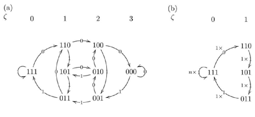
Our approach couples together consideration of the probability of the occurrence of various histories and the ranking in the performance of the strategies Lo2004. The history space consists of all the possible history bit-strings for a given value of . For , it includes bit-strings of ’s and ’s. Figure 2(a) shows the history space for , together with the possible transitions from one history to another. Each history constitutes a node in the history space. The transitions are marked by arrows together with the outcome necessary for making the transitions. It will prove convenient to group the possible history bit-strings for a given into columns, in the way shown in Fig. 2(a). Each column is labelled by a parameter , which is the number of ‘’s in the -bit history (histories) concerned. One immediate advantage of this labelling scheme is that the different states characterized by turn out to involve paths in a restricted portion of the full history space. For example, the state with is restricted to the portion of the history space, i.e. the history bit-string leads to an outcome of ‘1’ and hence persistent self-looping at the node in history space. The states with , , and correspond to different paths in the history space restricted to the and groups of histories, as shown in Fig. 2(b). The states with and have paths extended to include histories. The state with has paths that cover the whole history space (). In general, the deviation of from acts like a driving force in the history space that drifts the system towards an increasingly restrictive portion of the history space bounded by a smaller value of . One can also view this behavior as the system, in response to the global resource level , effectively avoiding certain nodes in the history space and hence avoiding particular patterns of historical outcomes.
V.2 Bit-string statistics of different states
As the game proceeds, the system evolves from one history bit-string to another. This can be regarded as transitions between different nodes (i.e. different histories) in the history space. For in the efficient phase, it has been shown savit that the conditional probability of an outcome of, say, ‘’ following a given history is the same for all histories. For , the result still holds for states characterized by . Note that a history bit-string can only make transitions to history bit-strings that differ by the most recent outcome, e.g. 111 can only be make transitions to either 110 or 111, and thus many transitions between two nodes in the history space are forbidden. In addition, these allowed transitions do not in general occur with equal probabilities. This leads to specific outcome (and history) bit-string statistics for a state characterized by .
We have carried out detailed analysis of the statistics of the outcomes following a given history bit-string for , and for each of the possible states over the whole range of . Table 4 gives the relative numbers of occurrences of each outcome for every history bit-string. For the state with , for example, the outcomes ‘’ and ‘’ occur with equal probability for every history bit-string, as in the MG. For the other states, the results reveal several striking features. It turns out that is given by the relative frequency of an outcome of ‘’ in the outcome bit-string, which in turn is governed by the resource level . For example, a ‘0’ to ‘1’ ratio of in the outcome bit-strings corresponds to the state with . In Table 4, we have intentionally grouped the history bit-strings into rows according to the label in Fig. 2. We immediately notice that for every possible state in the B-A-R model, the relative frequency of each outcome is a property of the group of histories having the same label rather than the individual history bit-string, i.e. all histories in a group have the same relative fraction of a given outcome. This observation is important in understanding the dynamics in the history space for different states in that it is no longer necessary to consider each of the history bit-strings in the history space. Instead, it is sufficient to consider the four groups of histories (for ) as shown in Fig. 2(a). Analysis of results for higher values of show the same feature.
For the state characterized by , the outcome bit-string is persistently ‘’ and the path in the history space is repeatedly 1111. Therefore, the path is restricted to the history labelled by and simply corresponds to an infinite number of loops around the history node 111. Since there is no ‘’ in the outcome bit-string, we will also refer to this state as state. The system is effectively frozen into one node in the history space. In this case, there are effectively only two kinds of strategies, which differ by their predictions for the history 111. The difference in predictions for the other () history bit-strings become irrelevant. Obviously, the ranking in the performance of the two effective groups of strategies is such that the group of strategies that suggest an action ‘1’ for the history ‘111’, outperforms the group that suggests an action ‘0’. For a uniform initial distribution of strategies, there are agents taking the action 0 and agents taking the action ‘1’, since half of the strategies predict 0 and half of them predict 1. To sustain a winning outcome of ‘1’, the criterion is that the resource level should be higher than the number of agents taking the action ‘1’. Therefore, we have for the state with that
| (1) |
and
| (2) |
These results are in agreement with the results obtained by numerical simulations. For , for . Note that Equations (1) and (2) are valid for any values of .
Table 4 shows that the states with , , have very similar features in terms of the bit-string statistics. They differ only in the frequency of giving an outcome of following the history of . Note that the and histories do not occur. The results imply that as the system evolves, the path in history space for these states is restricted to the two groups of histories labelled by and . The statistics show that the outcome bit-strings for the states with , and exhibit only one -bit in a period of , and bits, respectively. We refer to these states collectively as states, since the portion of allowed history space is bounded by the histories. Graphically, the path in history space consists of a few self-loops at the node 111, i.e. from 111 to 111, then passing through the group of histories once and back to 111, as shown in Fig. 2(b). The states with , , involve the other groups of histories and exhibit complicated looping among the histories. We refer to them collectively as higher (i.e. ) states.
VI The states
VI.1 Values of
We now proceed to derive an expression for the observed value of for the states. Recall that each strategy consists of a prediction or action for all of the -bit histories. An important idea is that for states corresponding to paths restricted to a certain portion of the history space, only that part of a strategy corresponding to the histories in question is being used in making decisions. Strategies that only differ in their predictions for the history bit-strings which do not occur (i.e. the avoided histories) are now effectively identical. In the context of the Crowd-Anticrowd theory johnson1; johnson2; johnson3, two previously uncorrelated strategies could now be correlated when viewed within this restricted history subspace.
As decreases, the system is allowed to explore a larger portion of the history space. The ranking in the strategies’ performance becomes more complicated. For the states, the paths in history space involve the () histories labelled by 0 and 1 (see Fig. 2(b)). For , only four out of a total of entries in a strategy corresponding to the histories ‘’, ‘’, ‘’, and ‘’ now matter. For general , there are histories with one ‘0’-bit: hence a total of () entries in each strategy now matter. For later discussions, it is useful to first classify all strategies into two groups according to their prediction for the history ‘11…1’ ( history). These strategies can further be classified according to their predictions for the histories. A strategy having bits predicting 1 and bits predicting 0 for the histories belonging to , can be labelled as (; , ) where is the prediction for the history. The first three columns in Table 5 show this classification of strategies for general values of describing the states.
For , the outcomes are no longer persistently ‘’, and the system explores both the and groups of histories. Assume that for just below , the outcome must be ‘’ for the histories, i.e. the system only visits the histories once in a cycle. Consider the case, for example. As time evolves, the system exhibits periodic visits to the histories. In each period, each history in occurs once and the history in occurs times. Among these occurrences of the history, the outcomes are ‘’ for timesteps and ‘’ for one timestep (Fig. 2(b)), since the system must go from ‘’ to ‘’ after loops in order to sustain the path. It turns out that paths in the history space for the , , and states () correspond to that shown in Fig. 2(b) with , , and loops at the history.
Since only different histories are involved, the performance of a strategy depends only on the predictions for this subset of histories. Consider the path in Fig. 2(b). The strategy labelled by predicts the correct outcome times for and times for , respectively, in going through the path once. In Table 5, we list the performance of the strategies labelled by according to the number of successful predictions (which reflects the VPs) in a closed path (see Fig. 2(b)) consisting of loops at history, i.e. a total of timesteps from to . It is important to note that there may be overlaps in strategies’ performance between the and groups of strategies for small values of , i.e. strategies with the label and may win the same number of timesteps in a cycle and hence belong to the same rank in performance of the strategies. For example for and , strategies labelled by and belong to the same rank in performance.
The number of turns around the history which is consistent with the condition of , is restricted to the range . This criteria is related to the number of overlapping performances between the and groups of strategies (see Table 5). Note that for , we have , i.e. strategies with do not have overlapping VPs with strategies with . This implies that the VPs of the strategies predicting ‘’ for the history in , are always higher than those predicting ‘’. This further implies that agents will take action ‘’ for the history if one of their strategies belongs to the category. For , there will then be agents taking the action ‘’. Since , the outcome must be ‘’. Therefore, the upper bound for the number of self-loops is , and thus . In other words, for paths with the system must have and the path in history space will be that of an infinite number of loops around history, i.e. the state. For , strategies in will perform worse than or equally well to those in for . As , strategies that predict more ’s should perform better. Therefore, leads to inconsistency and thus . Thus for the states, with the corresponding of overlapping groups of strategies being in the range . Since each possible allowed value of or gives one state, there are altogether possible states for a given .
The values of for the states can be readily found. For a given value of , the best performance among the strategies is to have correct predictions in a path consisting of () timesteps with loops at the history. Therefore, for the states
| (3) |
For , we have and hence . There are three states with , , and , exactly as observed in the numerical simulations.
VI.2 Resource levels at transitions
We now derive the critical values of the resource level at which transitions occur from one value of to another for the states. Note that the transition from the state to the state for and , occurs at as predicted in Eq.(2). The condition for transitions from to state is that the value of can no longer support loops at the history before giving an outcome of ‘0’ for the history 111. From Table 5, we note that the performance of the group of strategies becomes increasingly better than the group as increases, and the number of agents taking the action ‘1’ increases towards . Therefore, the highest number of agents who take the action ‘1’ and win will arise at the last turn among the loops where the history 111 is followed by an outcome ‘1’. Similarly, the lowest number of winning agents will be at the turn when the history 111 is followed by an outcome ‘0’, i.e. breaking away from the loops at 111.
The number of agents choosing the action ‘1’ given the history 111, is related to the number (and hence ) of overlapping performances among the and strategies. From Table 5, the number of correct predictions of a strategy in going through a path with loops at the history, is given by
| (4) |
For general values of , there are only histories which matter for the states. Therefore there are effectively different strategies, each of which represents a group of strategies. The number of effectively different strategies predicting for the history and having predictions of ‘1’ for the histories, is given by
| (5) |
for both and , where is the binomial coefficient.
The performance of the strategies can be ranked by a label , with and representing the best performing group of strategies. A general situation in which there are overlapping performances between the strategies and strategies, is shown in Table 6. For the states, the best performing strategies belong to the group and the worst performing ones belong to the group, with overlapping rankings in between where the allowed range of is . The ranking of the strategies is related to by the simple relation
| (6) |
For a given value of , there are a total of ranks. Therefore, the label is restricted to the range with given by
| (7) |
As the number of loops increases, decreases and the strategies spread more widely in terms of performance. It follows from Eqs. (5) and (6) that the number of effectively different strategies in rank- is given by
The fraction of rank- strategies among all the strategies is then given by
| (12) |
On the critical turn that determines the minimum value of for sustaining a certain state, only the strategies win. Using Table 6 together with Eqs. (5) and (6), the number of winning strategies is
The corresponding fraction of winning strategies among all strategies of rank-r is given by
Each agent uses the strategy in his possession which has the best performance record, i.e. the one having the ranking with smaller , in order to make a decision. Assuming a uniform initial distribution of any combination of strategies (with repetitions allowed) among the agents, the fraction of agents holding a rank- strategy as their best performing strategy is
| (20) |
with given by Eq.(12).
Each state corresponds to a specific value of allowed and hence an allowed . For a given or , the resource level needed to accommodate all the agents that take the action ‘1’ for the history, gives the criterion for the state:
| (21) |
Note that , , and are all -dependent (see Eqs.(7), (VI.2), and (21)). Equation (21) gives the lower bounds of for each of the states. Note that the lower bound for a state with a given is also the upper bound for the state with . For , , and , , and , Eq.(21) gives the lower bounds of , , and for the states characterized by , , and , respectively. These values are in excellent agreement with those obtained by numerical simulations (see Fig. 1(a) and Table 1). We note that our approach of focusing on strategy-performance ranking patterns and the fraction of strategies in each rank, represents a generalization of a similar approach Lo2004 that has already been successfully applied to the MG to cases in which some of the strategies have runaway VPs.
VII Discussion
We have studied numerically and analytically the effects of a varying resource level on the success rate of the agents in a competing population within the B-A-R model. We found that the system passes through different states, characterized either by the mean success rate or by the highest success rate in the population , as decreases from the high resource level limit. The number of states depends on details of the system such as the memory size and the number of strategies per agent . Transitions between these states occur at specific values of the resource level. For small values of , it is possible to explain these states by following the evolution of the performance of the strategies and the decision making dynamics of the system. More generally, we found that different states correspond to different paths covering a subspace within the whole history space. In the high resource level regime, namely , . The corresponding path in the history space is one that loops around the history ‘111…’ indefinitely. Just below the high resource level regime is a range of that gives states corresponding to the fractions . This result is in excellent agreement with that obtained by numerical simulations. For these states, i.e. the outcome series consists of one bit of ‘0‘ in a cycle of bits, the path in history space is restricted to those -bit histories with at most one-bit of ‘0’ and with loops around the ‘111…’ history. This identification of an active portion within the history space implies that only part of each strategy is being used. By considering the performance of the strategies within this restricted portion of the history space, the number of loops consistent with the states was found to be . The number of agents using a strategy that predicts the action ‘1’ given the history ‘111…’ increases as the number of loops increases. Thus a criterion on the resource level for sustaining a state of given can be derived. The results are again in excellent agreement with numerical results. After passing through the states, the system goes into states with more than one ‘0’-bit per cycle in the outcome series as is further reduced. These states correspond to paths that explore an increasingly larger portion of the history space. While our analysis can also be applied to these states, the dynamics and the results are too complicated to be included here.
A resource level that deviates from acts like a driving force in the history space. In response to this driving force, the system effectively adjusts its dynamics to occupy an increasingly restricted portion of the history space as increases. For , the system explores the whole history space by passing through trails that are almost Eulerian Jefferies1. The random initial distribution of strategies and the random initial history bit-string that started the system, provide the seed for the diffusive behavior which develops in the history space as the system evolves. In fact, results of numerical simulations for show that slightly increasing beyond has the effect of suppressing this random wandering through the history space, and instead locks the system into the Eulerian Trail. However opposing mechanisms can arise to counteract this driving force, thereby enhancing the diffusive behavior. For example, this can be achieved by allowing the agents the chance of using a strategy besides the best-performing one thermal1; thermal2 or by allowing some agents to opt out of the system occasionally larry1. Alternatively, the system can be biased through the initial strategy scores, or by introducing a specially prepared non-random initial allocation of strategies Jefferies1. It is this competition between the diffusive and driven behavior that gives the non-trivial global behavior in the B-A-R model and its variations. For this reason, the present B-A-R system provides a fascinating laboratory for studying correlated, non-Markovian diffusion on a non-trivial network (i.e. history space). This non-trivial diffusion is in turn strongly coupled to the non-random temporal patterns arising in the VP dynamics. We note that the present results could also be used to generalize the Crowd-Anticrowd theory in order to incorporate the effect of restricted history-space dynamics: this would then allow identification of an appropriate set of correlated, uncorrelated and anti-correlated strategies in order to implement the Crowd-Anticrowd theoretical expressions.
As a side-product, our analysis serves to illustrate the sensitivity within multi-agent models of competing populations, to tunable parameters. By tuning an external parameter, which we take as the resource level in the present work, the system is driven through different paths in the history space which can be regarded as a ‘phase space’ of the system. The feedback mechanism, which is built-in through the decision making process and the evaluation of the performance of the strategies, makes the system highly sensitive to the resource level in terms of which states the system decides to settle in or around. These features are quite generally found in a wide range of complex systems. The ideas in the analysis carried out in the present work, while specific to the B-A-R model used, are also applicable to other models of complex systems.
In closing, we remark that besides obtaining analytically the highest success rate and the criteria on the resource level , our treatment can also be extended to obtain the mean success rate for the states. The analysis is more complicated than that for obtaining . The procedure is to follow the evolution of the performance of the groups of strategies in each timestep through a path in the history space. The number of agents taking a particular action, and hence the number of winning agents, can be found from a strategies’ performance table like the one shown in Table 5. We have carried out the analysis for for , , and , and results are found to be in excellent agreement with numerical results. Our analysis can also be readily extended to consider connected populations in which agents have established links to connected neighbors for collecting additional information gourley; choe1; Lo2004. Quite generally, the effect of the links is to modify the number of agents using a strategy in a particular rank. For connected populations, an agent may use a strategy that he does not hold but has access to through his links. For an agent who uses the best performing strategy among his own strategies and those of his connected neighbors, the success rate behaves in a similar fashion as a function of as that reported here, only that the critical values of resource level at which transitions occur are shifted sonic. These results can be understood by incorporating the effects of the linkages into Eq.(20). Results for the B-A-R model in a connected population will be reported elsewhere sonic.
Acknowledgements.
This work was supported in part by the Research Grants Council of the Hong Kong SAR Government through Grant No. CUHK4121/01P. We acknowledge useful discussions with Ho-Yin Lee, Keven K. P. Chan, Charley S. Choe and Sean Gourley.References
- (1) For an overview of recent progress and activites in agent-based modelling of complex systems, see, for example, http://sbs-xnet.sbs.ox.ac.uk/complexity/ and http://www.ima.umn.edu/complex/.
- (2) N.F. Johnson, P. Jefferies, and P.M. Hui, Financial Market Complexity (Oxford University Press, 2003).
- (3) B. Arthur, Amer. Econ. Rev. 84, 406 (1994); Science 284, 107 (1999).
- (4) N.F. Johnson, S. Jarvis, R. Jonson, P. Cheung, Y.R. Kwong, and P.M. Hui, Physica A 258 230 (1998).
- (5) D. Challet and Y.C. Zhang, Physica A 246, 407 (1997); ibid. 256, 514 (1998).
- (6) See the website http://www.unifr.ch/econophysics/minority for updated information on the minority game.
- (7) For a review, see N.F. Johnson and P.M. Hui, cond-mat/0306516.
- (8) N.F. Johnson, S.C. Choe, S. Gourley, T. Jarret, and P.M. Hui, in Advances in Solid State Physics 44, edited by B. Kramer (Springer-Verlag, Heidelberg, 2004), p. 427.
- (9) N.F. Johnson, P.M. Hui, D. Zheng, and C.W. Tai, Physica A 269, 493 (1999).
- (10) D. Challet, M. Marsilli, and G. Ottino, cond-mat/0306445.
- (11) D. Challet, M. Marsili, and R. Zecchina, Phys. Rev. Lett. 85, 5008 (2000).
- (12) D. Challet, M. Marsili, and Y.C. Zhang, Physica A 294, 514 (2001).
- (13) N.F. Johnson, M. Hart, and P.M. Hui, Physica A 269, 1 (1999).
- (14) M. Hart, P. Jefferies, N.F. Johnson, and P.M. Hui, Physica A 298, 537 (2001).
- (15) D. Challet and M. Marsili, Phys. Rev. E 60, R6271 (1999).
- (16) M. Marsili, D. Challet, and R. Zecchina, Physica A 280, 522 (2000).
- (17) J.A.F. Heimel and A.C.C. Coolen, Phys. Rev. E 63, 056121 (2001).
- (18) J.A.F. Heimel, A.C.C. Coolen, and D. Sherrington, Phys. Rev. E 65, 016126 (2001).
- (19) D. Challet and M. Marsili, Phys. Rev. E 62, 1862 (2000).
- (20) T. Galla, preprint cond-mat/0406158.
- (21) R. Savit, R. Manuca, and R. Riolo, Phys. Rev. Lett. 82, 2203 (1999).
- (22) D. Zheng and B.H. Wang, Physica A 301, 560 (2001).
- (23) K. F. Yip, T. S. Lo, P. M. Hui, and N. F. Johnson, Phys. Rev. E 69, 046120 (2004).
- (24) P. Jefferies, M. L. Hart, and N. F. Johnson, Phys. Rev. E 65, 016105 (2002).
- (25) T. S. Lo, H. Y. Chan, P. M. Hui, and N. F. Johnson, Phys. Rev. E (2004), in press; see also preprint cond-mat/0406391.
- (26) S. Gourley, S.C. Choe, N.F. Johnson, and P.M. Hui, Europhys. Lett. (2004), in press; see also preprint cond-mat/0401537.
- (27) T. Chakraborty and P. Pietilainen, The Quantum Hall Effects: Integral and Fractional (Springer, Berlin, 1995).
- (28) M. Anghel, Z. Toroczkai, K. E. Bassler, G. Kroniss, Phys. Rev. Lett. 92, 058701 (2004).
- (29) S. C. Choe, N. F. Johnson, and P. M. Hui, Phys. Rev. E (2004), in press; see also preprint cond-mat/0405037.
- (30) T. S. Lo, K. P. Chan, P. M. Hui, and N. F. Johnson (unpublished).
- (31) A. Cavagna, J.P. Garraham, I. Giardina, and D. Sherrington, Phys. Rev. Lett. 83, 4429 (1999).
- (32) M.L. Hart, P. Jefferies, N.F. Johnson, and P.M. Hui, Phys. Rev. E 63, 017102 (2001).
- (33) S. Gourley, H.Y. Chan, P.M. Hui, and N.F. Johnson (unpublished).
| ‘1’-bits:‘0’-bits in a period | Range of | Period | |
|---|---|---|---|
| 8:8 | 510-600 | length 16 | |
| 12:5 | 600-620 | length 17 | |
| 17:6 | 620-640 | length 23 | |
| 5:1 | 640-695 | 111110 | |
| 6:1 | 695-745 | 1111110 | |
| 7:1 | 745-755 | 11111110 | |
| 1:0 | 755-1000 | 1 |
| Initial history = 0 | |||
| Timestep | outcome | ||
| (VP)(xy) | |||
| (initial history) | |||
| 1 | |||
| 2 | |||
| 3 | |||
| 4 | |||
| 5 | |||
| 6 | |||
| 7 | |||
| 8 | |||
| VP ranking pattern eventually repeats in four timesteps, with a 4-bit period of 1100 | VP ranking pattern eventually repeats in four timesteps, with a 4-bit period of 1110 | VP ranking pattern eventually repeats in every timestep, with the outcome being persistently ‘1’ | |
| ‘1’-bits:‘0’-bits in a period | Range of | ||
|---|---|---|---|
| 2:2 | 500-688 | ||
| 3:1 | 688-751 | ||
| 1:0 | 751-1000 |
| 0 | 1 | ||
|---|---|---|---|
| 000 | 1 | 1 | |
| 001 | 1 | 1 | |
| 010 | 1 | 1 | |
| 100 | 1 | 1 | |
| 011 | 1 | 1 | |
| 101 | 1 | 1 | |
| 110 | 1 | 1 | |
| 111 | 1 | 1 | |
| 8 | 8 | ||
| 0 | 1 | |
|---|---|---|
| 000 | 0 | 0 |
| 001 | 0 | 1 |
| 010 | 0 | 1 |
| 100 | 0 | 1 |
| 011 | 1 | 2 |
| 101 | 1 | 2 |
| 110 | 1 | 2 |
| 111 | 2 | 3 |
| 5 | 12 |
| 0 | 1 | |
|---|---|---|
| 000 | 0 | 0 |
| 001 | 0 | 1 |
| 010 | 0 | 1 |
| 100 | 0 | 1 |
| 011 | 1 | 3 |
| 101 | 1 | 3 |
| 110 | 1 | 3 |
| 111 | 3 | 5 |
| 6 | 17 |
| 0 | 1 | |
|---|---|---|
| 000 | 0 | 0 |
| 001 | 0 | 0 |
| 010 | 0 | 0 |
| 100 | 0 | 0 |
| 011 | 0 | 1 |
| 101 | 0 | 1 |
| 110 | 0 | 1 |
| 111 | 1 | 2 |
| 1 | 5 |
| 0 | 1 | |
|---|---|---|
| 000 | 0 | 0 |
| 001 | 0 | 0 |
| 010 | 0 | 0 |
| 100 | 0 | 0 |
| 011 | 0 | 1 |
| 101 | 0 | 1 |
| 110 | 0 | 1 |
| 111 | 1 | 3 |
| 1 | 6 |
| 0 | 1 | |
|---|---|---|
| 000 | 0 | 0 |
| 001 | 0 | 0 |
| 010 | 0 | 0 |
| 100 | 0 | 0 |
| 011 | 0 | 1 |
| 101 | 0 | 1 |
| 110 | 0 | 1 |
| 111 | 1 | 4 |
| 1 | 7 |
| 0 | 1 | |
|---|---|---|
| 000 | 0 | 0 |
| 001 | 0 | 0 |
| 010 | 0 | 0 |
| 100 | 0 | 0 |
| 011 | 0 | 0 |
| 101 | 0 | 0 |
| 110 | 0 | 0 |
| 111 | 0 | 1 |
| 0 | 1 |
| =0 history | =1 histories | number of correct predictions in a closed path with loops at =0 history | |||||||
| 1 | 0 | 1 | 2 | ||||||
| 1 | |||||||||
| 1 | |||||||||
| 1 | |||||||||
| 1 | |||||||||
| 0 | |||||||||
| 0 | |||||||||
| 0 | |||||||||
| 1 | |||
|---|---|---|---|
| 2 | |||
| ⋮ | ⋮ | ( strategies only) | |
| ⋮ | ⋮ | ⋮ | |
| r | |||
| ⋮ | ⋮ | ⋮ | (overlapping region) |
| ⋮ | ⋮ | ||
| ⋮ | 2 | ||
| 1 | ( strategies only) | ||