Defect generation and deconfinement on corrugated topographiesPreprint: APS/123-QED
Abstract
We investigate topography-driven generation of defects in liquid crystals films coating frozen surfaces of spatially varying Gaussian curvature whose topology does not automatically require defects in the ground state. We study in particular disclination-unbinding transitions with increasing aspect ratio for a surface shaped as a Gaussian bump with an hexatic phase draped over it. The instability of a smooth ground state texture to the generation of a defect is also discussed. Free boundary conditions for a single bump are considered as well as periodic arrays of bumps. Finally, we argue that defects on a bump encircled by an aligning wall undergo sharp deconfinement transitions as the aspect ratio of the surface is lowered.
pacs
Valid PACS appear hereI Introduction
The melting of a two dimensional crystal can occur continuously via two second order topological phase transitions characterized by the successive unbinding of dislocation and disclination pairs. At low temperatures, dislocations are suppressed due to their large energy cost, but as the temperature is increased, the entropy gained by creating defects overcomes their cost in elastic energy and dislocation unbinding occurs to reduces the overall free energy of the system Nelson and Halperin 1979; Kosterlitz and Thouless 1973; Young 1979. The quasi-long range order of the crystal is thus destroyed leading to an hexatic phase that still preserves quasi-long range orientational order. This phase can be characterized by a complex order parameter with six-fold symmetry. As the temperature is increased still further, an additional disclination-unbinding transition occurs and the hexatic order is finally lost in an isotropic liquid phase Nelson and Halperin 1979.
Experimental evidence for hexatic order and defect-mediated melting has been obtained in systems as diverse as free standing liquid crystal films Chou et al. 1998, Langmuir-Blodgett surfactant monolayers Knobler and Desai 1992, two-dimensional magnetic bubble arrays Seshadri and Westervelt 1991, electrons trapped on the surface of liquid helium Grimes and Adams 1979; D. C. Glattli and Williams 1998; Deville et al. 1984, two-dimensional colloidal crystals Murray; K. Zahn and Maret 1999 and self-assembled block copolymers Segalman et al. 2003.
The unbinding of defects in the plane is entropically driven and at low temperature defects are tightly bound. By contrast, on surfaces with non zero (integrated) Gaussian curvature, excess defects be present even at very low temperatures. The theory of topological defects in ordered phases confined to frozen topographies with positive or negative Gaussian curvature has been investigated previously; see, e.g., Sachdev and Nelson 1984; Nelson 1983; Nelson 2002. As a general rule, regions of positive or negative curvature (valleys, hills or saddles) lead to unpaired disclinations in the ground state, possibly screened by clouds of dislocations. These clouds can in turn condense into grain boundaries at low temperature. The predictions of recent studies of crystalline order on a sphere Bowick et al. a have been confirmed in elegant studies of colloidal particles packed on the surface of water droplets in oil Bausch et al. 2003. Investigations of the physics of defects in curved spaces have also been carried out for fluctuating geometries David et al. 1987; Nelson and Peliti 1987; Guitter and Kardar 1990; Park and Lubensky 1996. The dynamics of hexatic order on fluctuating spherical interfaces was studied in Ref. Lenz and Nelson 2003. Quenched topographies in the limit of small deviations from flatness were investigated in Ref. Sachdev and Nelson 1984 .
In the present work, we investigate topography-driven generation of defects on simple frozen surfaces with spatially varying Gaussian curvature whose topology does automatically enforce their presence in the ground state. We study in particular a two-dimensional ”bump” with a Gaussian shape and dimension large compared to the particle spacing. For such a hilly landscape, flat at infinity, the control parameter is an aspect ratio given by the bump height divided by its spatial extent. Consider a hexatic phase draped over such a bump. For small bumps, the ideal hexatic texture is distorted, but there are no defects in the ground state. As the aspect ratio is increased, we find that disclination pairs progressively unbind at in a sequence of transitions occurring at critical values of the aspect ratio. The defects subsequently position themselves to partially screen the Gaussian curvature. For bumps embedded in surfaces of sufficiently small spatial extent, a second instability of the smooth ground state needs to be considered. In this case, the energy stored in the field can be lowered by generating a positive defect at the center of the bump. Novel effects also arise when the hilly surface is encircled by an aligning circular wall that insures a rotation of the orientational order in the ground state. In this case, some of the positive defects required to match the curvature of the boundary are confined to a hemispherical cup centered on the bump, provided the aspect ratio is larger than a critical value . When is lowered below , the positive defects originally ”trapped” in the hemispherical cup start undergoing a series of sharp ”deconfinement transitions”, as they progressively migrate to new equilibrium positions dictated by boundary conditions and the finite system size. We also suggest possible ground states for periodic arrays of bumps, like those on the bottom of an egg carton.
A natural arena to experimentally study the interplay between geometry and defects is provided by thin copolymer films on SiO2 patterned substrates Kramer. Flat space experiments by Segalman have already demonstrated that spherical domains in block copolymer films form hexatic phases Segalman et al. 2003.
Our results for hexatics on frozen topographies also apply to other XY-like models, as might be appropriate for tilted surface-active molecules on curved substrates with interactions which favor alignment. The results are relevant as well to two-fold nematic order on frozen topographies. In both cases, we expect qualitatively similar defect unbinding transitions, although the equivalence becomes more exact in the one Frank constant approximation de Gennes and Prost 1993. Related results have been obtained recently for order on a torus Bowick et al. b. Even though the Gaussian curvature vanishes, defects appear in the ground state in the limit of fat torii, unless the number of degrees of freedom is very large.
The outline of this paper is as follows. In Section II, the relevant mathematical formalism is introduced and used to highlight similarities and differences between defects on surfaces of varying curvature and electrostatic charges in a non-uniform background charge distribution in flat space. As an example, we calculate the distorted, but defect-free, ground state texture of a hexatic confined to a surface shaped as a ”Gaussian bump” for aspect ratios below the first disclination-unbinding instability. In Section III, we investigate curvature-induced defect formation for an isolated bump and a periodic array of bumps. In section IV, defect deconfinement is discussed and in section V various experimental issues related to our analysis are highlighted along with some directions for future work. The development of the mathematical formalism is largely relegated to Appendices. In Appendix A the Green’s function for the covariant Laplacian is derived by means of conformal transformations. In Appendix B, we introduce a geometric potential whose source is the Gaussian curvature. In Appendix C, we present the general formula for the energy of textures with defects in terms of the two functions derived in Appendix A and B. We thus explore the existence of position-dependent defect self-interactions that arise from the varying Gaussian curvature. Finally, boundary effects are discussed in Appendix D.
II Hexatic order on a surface
II.1 Electrostatic analogy
The free energy for hexatic degrees of freedom embedded in an arbitrary frozen surface can be written as
| (1) |
where is a set of internal coordinates, is a unit vector in the tangent plane, is the covariant derivative with respect to the metric of the surface and is the infinitesimal surface area Nelson and Peliti 1987; David et al. 1987; Park and Lubensky 1996; David. The generalization to systems with a p-fold symmetry is straightforward provided that the one Frank constant approximation is used and the consequences of the uniaxial coupling neglected de Gennes and Prost 1993. This choice of free energy implies that the minimal energy configuration will be given locally by neighboring vectors which differ only by parallel transport. The curvature of the surface induces ”frustration” in the texture. In fact, by Gauss’ ”Theorema egregium” Struik 1961; Kamien 2002, tangent vectors parallel transported along a closed loop are rotated by an amount equal to the Gaussian curvature integrated over the enclosed area. On a sphere, for example, the hexatic ground state always has twelve excess disclinations as a result of this frustration Nelson 1983; Lubensky and Prost 1992. More generally, the sum of the topological charges on any closed surface is equal to the integrated Gaussian curvature.
By introducing a local bond-angle field , corresponding to the angle between and an arbitrary local reference frame, we can rewrite the hexatic free energy introduced in Eq.(1) as:
| (2) |
where , is the determinant of the metric tensor and is the spin-connection whose curl is the Gaussian curvature David; Kamien 2002. The spin connection can be viewed as a ”geometric vector potential”. A free energy like Eq.(2) also describes the charged Cooper pairs implicit in the London theory of a superconductor well below . In the superconductor analogy, the Gaussian curvature plays the role of a (spatially varying) external magnetic field. For the problem considered here, however, there are interesting new nonlinear effects associated with spatial variations in the metric.
A detailed analysis of the free energy of Eq.(2) for a bumpy surface with free and circular boundary conditions is presented in Appendices (C) and (D). Here we only sketch the main steps and conclusions. The free energy can be readily converted into a Coulomb gas model by using the relation
| (3) |
where is the covariant antisymmetric tensor, is the Gaussian curvature and is the disclination density with defects of charge at positions . The final result is an effective free energy whose basic degrees of freedom are the defects themselves Park and Lubensky 1996; Bowick et al. a:
| (4) |
where is defined in Eq.(3). The Green’s function is calculated (see Appendix A) by inverting the Laplacian defined on the surface
| (5) |
and we have suppressed for now defect core energy contributions which reflect the physics at microscopic length scales. Eq.(4) can be understood by analogy to two dimensional electrostatics, with the Gaussian curvature (with sign reversed) playing the role of a non-uniform background charge distribution and the topological defects appearing as point-like sources with electrostatic charges equal to their topological charge . As a result, the defects tend to position themselves so that the Gaussian curvature is screened: the positive ones on peaks and valleys and the negative ones on the saddles of the surface. However, this analogy does neglect position-dependent self-interactions Vitelli and Turner, but since these are quadratic in the charge they are negligible for hexatics. Hence positive disclinations of minimal topological charge continue to be attracted to positive curvature (see Appendix C).
More generally, we can consider p-fold symmetric order parameters with minimum charge defects . The case corresponds to tilt order of absorbed molecules and describes nematics. The cases and describe tetradic and hexatic phases respectively Lubensky and Prost 1992. Strictly speaking, Eq.(1) only describes the cases and in the one-Frank-constant approximation de Gennes and Prost 1993. Most of our discussion focuses on topography-driven transitions on a model surface shaped like a bell curve or ”Gaussian bump” (see Fig. 1),

but the same mathematical approach can be readily carried over to study arbitrary surfaces of revolution that are topologically equivalent to the plane. Furthermore, we do not expect the results of this analysis to depend qualitatively on the azimuthal symmetry of the surface, which is assumed purely for reasons of mathematical convenience.
Points on our model surface embedded in three dimensional Euclidean space are specified by a three dimensional vector given by
| (6) |
where and are plane polar coordinates in the plane of Fig. 1. It is useful to characterize the deviation of the bump from a plane in terms of a dimensionless aspect ratio
| (7) |
The two orthogonal tangent vectors and can be normalized to define the Vierbein (orthonormal basis vectors) and respectively. The components of the spin connection introduced in Eq.(2) are given by David; Kamien 2002. This leads to a vanishing radial component and
| (8) |
where the important -dependent function (see Fig. 2) is defined by

| (9) |
and it is equal to the radial component of the diagonal metric tensor, ,
| (10) |
Note that the entry is equal to the flat space result in polar coordinates while is modified in a way that depends on but tends to the plane result for small and large , as illustrated in Fig. 2.
The Gaussian curvature for the bump is readily found from the eigenvalues of the second fundamental form Dubrovin et al. 1992,
| (11) |
Note that controls the order of magnitude of and that changes sign at (see Fig. 1b). The integrated Gaussian curvature inside a cup of radius centered on the bump is
| (12) |
which vanishes as . Eq.(12) also shows that the positive Gaussian curvature enclosed within the radius (see Fig. 1) approaches for , half the integrated Gaussian curvature of a sphere.
II.2 Defect free texture
For small values of the aspect ratio , the minimal energy texture for the hexatic will be free of defects. The ground state configuration satisfies the differential equation
| (13) |
which results from minimizing the free energy in Eq.(2) with respect to the field for fixed . When expressed in terms of the coordinates in Eq.(6), the solution of Eq.(13) reads:
| (14) |
where is an arbitrary constant. The smooth ground state texture is thus obtained if the director forms an angle with respect to the spatially varying basis vector . Note that a solution of the form represents a defect of charge in this ”rotating” system of coordinates.
As an illustration, consider the projection on the plane of the minimal energy texture of an XY model () as shown in Fig. 3.

The arrows represent the orientation of tilted molecules on this surface in the one Frank constant approximation. The field clearly displays strong frustration along a direction determined by the choice of the constant in Eq.(14). If the bump is positioned within two very distant walls parallel to the y-axis which impose tangential boundary conditions on the molecular tilts, the ”preferred” direction will be along 11 1 In case walls are present, the free solution of Eq.(14) is slightly modified to account for the new boundary conditions. This is accomplished by the method of images or conformal transformations Smirnov 1964.. The texture displayed in Fig. 3 can be interpreted as resulting from embryonic pairs of defect dipoles along the line . The distortion energy of this ground state is given by:
| (15) |
This expression can be evaluated for an infinitely large system by using Eq.(14) and the explicit form of the spin connection derived in Section II.1, with the result:
| (16) |
It follows from Eq.(16) that the ground state energy is a monotonically increasing function of the aspect ratio, proportional to for small . As we shall see, for large enough , it can be energetically preferable to reduce this energy by introducing defect pairs into the texture. It is convenient to rewrite Eq.(15) in terms of the Gaussian curvature and the Green function discussed in Appendix A David
| (17) |
This result is what one obtains by setting all in Eq.(4). The details of the mathematical derivation are relegated to Appendix C.
Although this result correctly represents the zero temperature limit of the vector model, corrections may be appropriate to describe the physics of ordered phases at finite temperature. ”Spin-wave” excitations (i.e., quadratic fluctuations of the order parameter about the ground state texture) can be accounted for by integrating out the longitudinal fluctuations around the ground state configuration . By letting in Eq.(2) and using Eq.(3) we obtain David et al. 1987; Park and Lubensky 1996:
| (18) |
The longitudinal variable appears only quadratically in and the trace over can be explicitly performed with the result Polyakov 1981:
| (19) |
where is the Liouville action,
| (20) |
The first term in this expression is a constant proportional to the fixed surface area of the frozen topography and will be suppressed in what follows. The remaining term causes a shift in the coupling constant appearing in Eq.(17) from to David et al. 1987; Park and Lubensky 1996. This ”entropic” correction to the coupling constant at finite temperature also arises when defects are present.
The energy in Eq.(17) represents an intrinsic, irreducible energy cost of geometric frustration for textures without defects. As we shall see, defects can reduce this frustration. However, for small values of the energy cost of this frustration will still be lower than the core energies associated with the creation of the unbound defects and the work necessary to tear them apart.
II.3 Energetics of defect pairs on a Gaussian bump
A quantitative understanding of the energetics of defects on a fixed topography is essential to calculate the critical value(s) of the aspect ratio above which defect-unbinding becomes energetically favorable. The first step is to calculate the Green’s function that governs the ”coulombic” interaction among defects and between each defect and the Gaussian curvature. The inversion of the curved space Laplacian can be more easily accomplished by employing a set of ”isothermal coordinates”, such that the resulting Green’s function reduces to the familiar logarithm of two dimensional electrostatics. As shown in Appendix A the final result in terms of the original polar coordinates reads:
| (21) | |||||
where the function can be thought of as a radial coordinate in the conformal plane resulting from adopting an isothermal set of coordinates (see Appendix A)
| (22) |
and is the -dependent function introduced in Eq.(9). The constant depends on the physics at short distances, which is discussed in Appendix A.
The Green function in Eq.(21) corresponds to free boundary conditions at infinity and preserves the cylindrical symmetry of the metric. It differs from the familiar result in flat space by a non-linear radial stretch corresponding to a smooth deformation of the bump into a flat disk. This Green’s function determines an attractive interaction for the defect dipole pair. However, the Gaussian curvature of the bump also generates a geometric potential that tries to pull the disclination dipole apart. This geometric interaction arises by combining cross terms between and in Eq.(4) with the position dependent self-interactions derived in Appendix C. The resulting interaction between defects and the Gaussian curvature takes the simple form
| (23) |
where the geometrical potential is defined as
| (24) |
The minus sign in front of this geometric potential insures that defects of topological charge between zero and are attracted by regions of positive Gaussian curvature Vitelli and Turner. For defects with a large topological charge of , the sign of the geometric interaction, , is reversed and, and defects of either sign are pushed away from the bump. This scenario does not affect the geometry-driven defect formation discussed in this paper that relies on disclinations whose charge is well below . However, as a result of the position-dependent self interactions, is no longer symmetric under the change , as one would expect on the basis of the electrostatic analogy. The effect of this asymmetry is small for hexatic order but it increase for liquid crystals with p-fold order parameter, as decreases (see Ref. Vitelli and Turner, and references therein).
Gauss’ law generalized to curved surfaces (see Appendix B) insures that the geometric force experienced by a defect of charge with radial coordinate will be determined only by the net curvature enclosed in a circle of radius centered on the top of the bump. The resulting ”electric field” is radial as expected from electrostatics and is proportional to the gradient of the geometric potential, which for a Gaussian bump takes the form (see Appendix B)
| (25) |
For small values of the aspect ratio the potential in Eq.(25) can be approximated by
| (26) |
The resulting force is linear for small (i.e. near the top of the bump) and decays like for . As the aspect ratio increases, the force generated by the curvature can overcome the attractive force binding the defect pair which varies logarithmically for short distances. As a result, oppositely charged defects that were originally tightly bound can be separated.
This argument, however, neglects another complication resulting from the curvature of the surface: as the aspect ratio is increased, the Green’s function in Eq.(21) and hence the force binding the defects together increases. We illustrate this point in Fig. 4 for the special case of a positive defect pinned right on top of the bump and a negative one free to move downhill at . Upon invoking Equations (4) and (21), the potential binding the pair, , can be written down exactly as:
| (27) | |||||
The first term is the flat space Green’s function and we have added two disclination core energies. The last term represents a ”curvature correction” that has the same functional form of the geometric potential in Eq.(25), but it represents a distinct contribution to the total free energy. As discussed in Appendix B, the pair potential energy, , can be understood by applying a generalized Gauss’ Law to the bump to determine a force which is equal to . The potential follows by integrating this force along the bump with the length element .
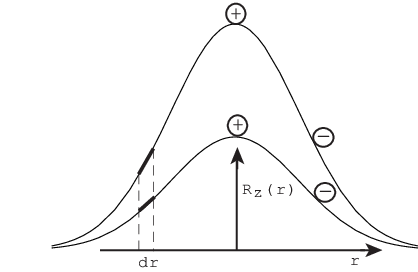
Although the force is independent of the aspect ratio, the length element grows with (see Fig. 4), which makes the pair more energetically bound for larger values of . A careful calculation of these effects (including the contribution associated with the position-dependent self-energies) reveals that the geometric force still overcomes the binding interaction for sufficiently large values of .
An estimate of the critical value of for which the dipole unbinds can be obtained by comparing the minimal free energy of the smooth frustrated field arising from Eq.(17) with the free energy in the presence of defects. The latter, as follows from Eq.(4), is composed of three contributions: the interactions among the defects, the interaction between the defects and curvature as given by Eq.(23) and the Gaussian curvature self-interaction. The latter is equal to the minimal free energy of the smooth frustrated field and is renormalized at finite temperature in the same way. (Associated with the cutoff is a microscopic core energy, , that we expect to be of the defect position on the bump, as long as the radius of curvature is much greater than any microscopic length scale.) The remaining two contributions are not renormalized by thermally induced spin wave fluctuations Park and Lubensky 1996. As shown in Appendix C, the difference in free energy of a defected texture described by Eq.(4) relative to the defect-free result Eq.(17) can be written as:
| (28) |
where we have assumed overall charge neutrality for the defect configuration. The subscript in indicates that a constant microscopic core radius has been absorbed in the definition of the Green function so that the argument of the logarithm in Eq.(21) becomes dimensionless, as in Eq.(102),
| (29) |
This microscopic cutoff corresponds to a constant core radius for each defect and it is of the order of the spacing between the microscopic degrees of freedom. The sum of microscopic core energies in the fourth term of Eq.(28) needs to be fixed phenomenologically or from models that go beyond simple elasticity theory Kleman and Lavrentovich 2003. Note that both and depend on . If becomes sufficiently large so that is less than zero, one or more disclination dipoles unbind in the hexatic phase at a sequence of critical values . The analogous defects in XY-model textures of tilted liquid crystal molecules would be vortex pairs.
III Curvature induced defect generation
III.1 Onset of the defect-dipole instability
If a dipole is created, say, along the line of zero Gaussian curvature, the positive disclination will be pulled towards the center by the positive curvature while the negative one will be repelled into the region of negative curvature.

The net result is a reduction of the total free energy of the order of the depth of the potential well since the logarithmic binding energy is approximately constant compared to the geometric potential. An approximate analytical treatment is obtained by assuming that the positive defect sits right at the center of the bump and the negative one at a distance of the order of . The validity of this approximation scheme can be checked by numerically minimizing the energy with respect to the position of the defects, as discussed in Section (III.2). We assume charge neutrality so that the two defects have equal and opposite topological charges of magnitude . For order parameters with a p-fold symmetry, the minimal topological charge is . The approximate free energy cost to generate this defect pair then follows from Equations (25),(27) and (28):
| (30) | |||||
The internal consistency of the formalism can be checked by investigating the limit . As the negative defect approaches the positive one at the center of the bump, we have and the energy tends to the expected flat space result .
The equilibrium position of the negative defect turns out to be for equal to a few , so the terms containing in Eq.(30) can be dropped as a first approximation because decays exponentially (see Fig. 5):
| (31) |
To estimate the critical value of the aspect ratio for which the first dipole unbinds, let and solve for in Eq.(31). Because a different choice for the core energy can be accounted for by rescaling the core size in Eq.(31), the condition for unbinding is
| (32) |
with
| (33) |
If we know and , the critical aspect ratio can be obtained from inspection of Fig. 6 where is plotted as a function of .

The Taylor expansion of derived in Eq.(26) gives to leading order in . Inspection of Fig. 6 shows that this approximation works sufficiently well even for aspect ratios of order unity. Upon substituting for into Eq.(32), we obtain an estimate of how depends on :
| (34) | |||||
Note that a critical height for defect unbinding is predicted for fixed with defect charge for all integer values of p. The validity of this approximate relation is tested in Section III.2.
The continuum theory adopted here is valid in the limit . If can be neglected compared to , the defect unbinding instability is triggered when the energy gain derived from letting the defects screen the Gaussian curvature (approximately given by ) overcomes the work needed to pull them apart a distance . This work, of order , increases very slowly with large , hence the continuum approximation can be satisfied while keeping the work finite. Note that the result does not depend on the size of the system because we assume overall disclination charge neutrality and the assumption that . In this limit, boundary effects can be ignored provided that they do not impose a topological constraint on the phase of the order parameter. An aligning outer wall in a circular hexatic sample, for example, would force the bond angle field to rotate by , leading to six defects in the ground state even in flat space. The interesting physics which results is addressed in Section IV.
III.2 Numerical investigation of defect-unbinding transitions
The disclination unbinding transitions can be investigated more quantitatively by minimizing numerically in Eq.(28) with respect to the positions of the defects. The aspect ratio above which becomes negative corresponds to the threshold value (analogous to a first order transition) for which the singular field is energetically favored with respect to the smooth texture of Fig. 3. We emphasize that the energy landscape can have two minima. The first occurs when two oppositely charged defects form a closely bound dipole (with separation of the order of the cutoff ) and hence annihilate each other leaving a smooth texture. The second minimum corresponds to an unbound pair (with separation of a few ) and it disappears when the geometric force is too weak to overcome the binding force of the pair. This scenario occurs for a value of characteristic of the geometry of the substrate above which the formation of an unbound dipole is possible, albeit energetically unfavored (see Fig. 7).

As is increased above , the smooth-texture minimum becomes metastable and the unbinding of a defect pair is the most likely scenario.
It is useful to parameterize in terms of the dimensionless radial coordinates . The geometric potential is defined in Eq.(60) as a function of , , where
| (35) |
In order to write the defect-defect interaction in terms of the dimensionless radial coordinate , we introduce a new function defined by
| (36) | |||||
where Eq.(59) was used in the last step. We can now transform by eliminating in favor of . Thus we have using Equations (102) and (63)
| (37) | |||||
where we have exploited charge neutrality and Eq.(103). The free energy minimized with respect to the positions of the defects, , can now be written, according to Eq.(28), as
| (38) |
where
| (39) | |||||
Note that in the second term in Eq.(38) the core energy of each defect has been absorbed in the modified core radius , as defined in Eq.(33). This generates an energy cost for unbinding that can be overcome if assumes sufficiently large negative values. Hence it is sufficient to study numerically how varies as a function of a single parameter, eg. . As an illustration of this approach, we study explicitly the unbinding of one and two disclinations pairs leading to the ground states represented schematically in Fig. 8.

The smooth ground state becomes unstable to the formation of one defect dipole first. The critical aspect ratio above which this scenario occurs can be determined with the aid of Fig. 9

where the function introduced in Eq.(39) is plotted as a function of the aspect ratio. From Eq.(38) we see that is determined by
| (40) |
For and , we obtain a critical aspect ratio . As a comparison, the approximate condition derived in Eq.(32) gives when used in conjunction with Fig. 6. The rougher estimate in Eq.(34) leads (for ) to . This discrepancy is easily understood considering that Eq.(34) was derived by means of a low expansion.

The critical aspect ratio is too low for the two-dipole defect configuration to become energetically favorable with respect to the smooth ground state. Indeed, inspection of Fig. 10 reveals that the critical aspect ratio for which the ”two-dipole instability” sets in is approximately equal to for the same choice of parameters used in the single pair case. Note that, in the presence of two dipoles, the energy cost arising from the second term in Eq.(38) is twice as large because there are four defects rather than two. However, for generating two dipoles becomes more energetically favored than a single dipole (see Fig. 11). The approach illustrated here can be used to calculate a cascade of defect unbinding instabilities at critical aspect ratios involving higher number of dipoles and their equilibrium configurations in the ground state. Note that the unbinding eventually stops since the integrated Gaussian curvature in the top cup cannot exceed . We expect the qualitative features of our analysis to be independent of the exact shape of the bumpy substrate although the specific values depend on the geometry and the choice of the microscopic parameters and . Finally, we emphasize that the curvature-induced unbinding is similar to a first order transition and occurs for rather pronounced deviations from flatness (ie. large ).

III.3 Single vortex instability
The unbinding of defect pairs may not be the most likely scenario if the size of the system is sufficiently small. In this case, the creation of a single vortex at the center of the bump may become energetically favorable for lower aspect ratios than required by the defect dipole instability. The equation for the bond angle field for a single defect of charge at the center of the bump is given by:
| (41) |
where the bond angle is measured with respect to the rotating basis vectors corresponding to the polar coordinates discussed in Section II.2. Upon substituting in Eq.(2) and subtracting the free energy corresponding to the defect-free texture we obtain:
| (42) | |||||
where was added by hand. The same result is obtained by using the more general formalism developed in Appendix D. Indeed, by letting the position of an isolated defect tend to the center of the bump in Eq.(127) we obtain the energy of the singular field in the case of free boundary conditions and the result matches Eq.(42). As discussed in Appendix D, a defect located at is attracted to the boundary at for free boundary conditions. One can think of this interaction as resulting from an image defect of opposite sign behind the edge of the sample at position such that the following relation holds in terms of the conformal radius
| (43) |
This result can be understood by analogy to the familiar electrostatic problem of a charged line located a distance from the center of a cylindrical grounded conductor whose axis is parallel to it Panofsky and Phillips 1962. The analogy becomes precise if one lets as explained in Appendix D.
If the geometric potential is not strong enough (as in the flat space limit ), the defect will migrate to the edge of the sample and annihilate with its image leaving a smooth field. On the other hand, when the aspect ratio is sufficiently large, the defect can lower its energy by sitting at the center of the bump. Comparison of Eq.(42) with Eq.(31) shows that, unless , the energy of the single vortex instability will be lower or at least comparable to the unbinding of a defect dipole. In fact, the threshold that needs to exceed to trigger the single defect instability is easily obtained if the values of the geometric potential at the origin are tabulated for different aspect ratios, as illustrated in Fig. 5. The condition for single vortex generation reads
| (44) |
Using the same method adopted to derive Eq.(34) we obtain an estimate of how depends on (compare with Eq.(34)):
| (45) |
The single vortex instability is reminiscent of vortex generation in rotating superfluid helium with playing the role of the angular speed . For a volume of helium contained in a cylindrical vessel of radius and rotating uniformly with constant angular speed, the critical value above which defect generation occurs is given by Vinen
| (46) |
where is the magnitude of the quantum of circulation and the core radius 22 2 A similar mechanism applies to superconductors in a uniform magnetic field.. Note that decreases as increases, unlike which diverges logarithmically. Thus, the single defect instability studied here is a finite size effect. In contrast, the disclination unbinding studied earlier in this section does not depend on the system size because of charge neutrality. Hence the thermodynamic limit can be safely taken, provided the characteristic length over which the curvature varies (ie. ) is not too large compared to (see Eq.(34)).
In considering the case of small system size, it is important to keep in mind two assumptions implicit in the present treatment. The radius of curvature must be much larger than the core radius everywhere for the continuum approach to be valid, that is . Additionally, the Gaussian curvature must be vanishing small at the edge of the system which requires to be larger than a few .
III.4 Lattice of bumps, valleys and saddle points
In some experimental realizations perhaps modelled on those of Ref. Segalman et al. 2003 the topography will be periodic. In this Section we discuss qualitatively how the results described above generalize to a 2-dimensional lattice of bumps with variable aspect ratio for both square and triangular lattices. A more quantitative approach to this problem would involve finding conformal set of coordinates for periodic boundary conditions. This is possible in principle but more involved since cylindrical symmetry is now lost. Nonetheless, the intuition gained by studying the single bump allows us to make some guesses for the ground state. We first note that the geometric potential generated by the lattice of bumps is not simply the superposition of results for single bump potentials. This is caused by the non linear relation between the surface height and the Gaussian curvature acting as a source for the geometric potential. To explore this point further, consider what happens when four bumps are placed at the vertices of a square. At the center of the square a minimum of the height function occurs corresponding to a region of positive Gaussian curvature. This effect is particularly acute for , where is the bump spacing. In general interference between bumps creates a dual lattice of valleys. A similar breakdown of the superposition principle arises for triangular lattices.

As the aspect ratio of hilly landscapes such as those shown in Fig. 12 is increased, defects can be created to screen the Gaussian curvature. Their positions can be guessed by considering a unit cell of the lattice such that the integrated Gaussian curvature vanishes. For a square lattice, we conjecture that the first topography induced transition is associated with the appearance of positive defects at the top of the bumps and negative ones half way between them in the vertical or horizontal direction (see Fig. 12). This two-fold degeneracy is compatible with the symmetry of the lattice and analogous to the freedom in choosing the axis along which the first disclination-dipole appears on the single bump. The negative defects are shared between two adjacent cells while the positive ones are shared among four cells thus ensuring overall charge neutrality. As the value of increases even more, one might expect an additional positive defect appears in the valley located at the center of each cell and two additional negative defects shared with the adjacent cells are created between the bumps at right angles to the direction discussed above (see Fig. 12).
For the triangular lattice, we conjecture that the first transition corresponds to positive defects on top of the bumps and negative ones between the bumps along one of the three axis of symmetry of the unit cell. As the value of the aspect ratio is increased, additional positive defects appear on the six minima of the surface and negative ones are generated along the remaining two axes of symmetry of the unit cell (see Fig. 12). A simple count of the total defect charges enclosed in the unit cell shows that this scenario also satisfies the requirement of defect charge neutrality.
IV Defect Deconfinement
With potential experiments in mind Kramer, it is interesting to consider the case of hexatic order on a bump encircled by a circular wall of radius which aligns the hexatic bond angles. As a simple model, imagine an array of hexagons which locally achieve a common orientation tangential to the wall (see Fig. 18b). The hexatic order parameter will thus rotate by upon making a circuit of the wall, insuring that at least six defects of ”charge” must be included in the ground state for all values of the aspect ratio. These boundary-condition induced defects will interact with the Gaussian curvature of the bump and with the wall. The defects contribute large (constant) self energies of the form that dominate the total energy for sufficiently large systems. Since must be equal to , the energy is minimized when the defects split up into the smallest possible charges.
The equilibrium defect configuration must minimize the free energy taking into account the confining potential generated by the Gaussian curvature and the interactions of the defects with the boundary and among themselves. The repulsive force exercised by the wall on a defect located at in the conformal plane can be computed by placing an image defect of same charge outside the wall at position . The mathematics resembles the problem of finding the magnetic field of a line current located at a given distance from the center of a cylinder of high permeability material and whose radius is greater than Panofsky and Phillips 1962. The analogy is complete upon performing the change of coordinates and identifying the gradient of the bond angle with the magnetic field. This is explained in detail in Appendix C and D where we introduce a conjugate function analogous to the vector potential that simplifies the analysis of this problem. Thus, each of the defects will also interact with an equal number of image defects. This situation can be described mathematically by deriving an appropriate Green’s function that includes the images, as discussed in Appendix D (see Eq.(122)). The resulting free energy reads:
| (47) | |||||
where is defined in Eq.(17) and the Green’s function is given by
| (48) |
The last term accounts for the interaction with the image defects and the superscript indicates Neumann boundary conditions on an appropriate potential function. Here, we use scaled coordinates in the conformal plane . The interaction of the defects with the curvature is not affected by the presence of the distant wall.
To provide an illustration of the combined effect of curvature and boundary conditions on tangential vector order, we first consider the simpler case of a nematic order parameter with periodicity equal to . This simplified model neglects differences in the elastic constants for bend and splay and does not incorporate any effect due to the uniaxial coupling of the nematogens to the curvature. In this case, minimization of the logarithmically diverging part of the free energy (fourth term in Eq. 47) suggests that there will be only two disclinations of charge displaced along a radial direction (see Fig. 13b). By applying Eq.(47), we can parameterize the energy of the system in terms of the scaled radial coordinates, and of the two disclinations. The resulting energy landscape is plotted in Fig. 13 (for and ) and clearly reveals two minimal-energy configurations. The first minimum corresponds to one disclination confined at the top of the bump (slightly shifted from the center) and the other at a radial distance approximately 70% of (see Fig. 13b bottom panel). The second minimum corresponds to a fully deconfined state with both disclinations placed symmetrically at approximately 67% of (see Fig. 13b top panel). As the aspect ratio is raised even further, the saddle in the energy landscape of Fig. 13a becomes a minimum corresponding to a configuration in which both disclinations are confined in the cup of positive Gaussian curvature by the geometric potential.

As illustrated in Fig. 14, there is a critical value of the aspect ratio, , above which it is energetically favorable for the system to have one disclination confined at the top of the bump. For the fully deconfined configuration becomes energetically favorable, but the two minima can still coexist. As is decreased even further, the repulsion between the two disclinations overcomes the confining force of the geometric potential and makes the second minimum in Fig. 14a (corresponding to the partially confined configuration) disappear altogether. This ”spinodal point” occurs for on the Gaussian bump. The specific values of the critical aspect ratios are geometry dependent, but the generic mechanism of deconfinement depends only on a large separation of the length scales and that control the interaction with the curvature and the boundary respectively.

The analysis for the hexatic case is complicated by the fact that more defect configurations are possible when six defects are present. We start by noting that even in flat space () there are two natural low energy defect configurations with high symmetry: the ground state corresponding to the six defects sitting at the vertices of an hexagon and a higher energy state given by a pentagonal distribution of defects with the sixth defect sitting at the center of the circular sample (see Fig. 15b). As the aspect ratio is raised, the pentagonal arrangement becomes energetically favored since it pays to have a defect confined in the (geometric) potential well at the origin (see Fig. 15a). To study the transition, it is useful to derive expressions for the energy of the two defect configurations as a function of the radius of the outer defect ring . Every defect (except the one at the origin, possibly) has the same scaled coordinate and the angles between two defects are integer multiples of where is the number of defects in the outer ring ( for the pentagon and for the hexagon). In this case, the sums involved in the first (interaction) term in Eq.(47) can be efficiently evaluated using the following identity:
| (49) |
Upon using Eq.(49) with and to evaluate the sums arising from the first and the second term of the Green’s function in Eq.(48) respectively, we obtain the free energy for the hexagonal configuration:
| (50) | |||||
The free energy for the pentagonal configuration is readily obtained after similar manipulations
| (51) | |||||
Note that these manipulations are very similar to the ones necessary to describe superfluid helium in a cylinder of radius Hess 1967. In fact, the superfluid problem is analogous to the case of hexatic order with boundary conditions on a circular boundary of radius (see Appendix D). The rather unusual form of the argument of the logarithm in Equations (50) and (51) arises from the sum over the image defects whose positions depend non-linearly on the position of the defects themselves.
Minimization of Equations (50) and (51) with respect to fixes the distance of the outer defects. The resulting minimal energies and are plotted as a function of in Fig. 15a.

The critical value , for which can be easily estimated by realizing that is approximately independent of because the disclinations are far from the bump. On the other end, decreases with because the confined disclination is trapped in a potential well whose depth is approximately given by (see the second term of Eq.(51) and the low expansion for derived in Eq.(26)). The critical aspect ratio, , for which the deconfinement transition occurs can be estimated by setting the depth of this potential well equal to the energy difference between the hexagon and pentagon configurations in flat space. The latter can be read off from the energy diagram in Fig. 15a and the result is approximately which leads in agreement with the value indicated in Fig. 15a.
As the aspect ratio is raised even further, less symmetric defect configurations become energetically favored corresponding to a larger number of disclinations confined in the cup of positive Gaussian curvature. For example, when two disclinations are confined within , the outer defect ring is given by four defects approximately located at the vertices of a square. We note that these defect configurations cease to exist at low aspect ratios because they require the geometric potential to overcome the strong repulsive interaction between the confined defects. As discussed earlier for Fig.(14), the actual values of the aspect ratios involved depend on the specific geometry of the substrate. However the basic mechanism behind the deconfinement transition is more general.
Note that, as increases, the geometric mechanism of defect dipole unbinding discussed in the last section may also set in. Because of the presence of one or more positive defects at the top of the bump, the critical aspect ratio necessary to unbind one dipole will be larger than what was calculated before. If dipole unbinding does occur, the new defects will ”decorate” the existing patterns by adding new positively charged disclinations in the region of positive Gaussian curvature and expelling the negative ones in the external region of the bump () where the Gaussian curvature is also negative (see Fig.1).
V Conclusion
We have discussed how the varying curvature of a surface such as a ”Gaussian bump” can trigger the generation of single defects or the unbinding of dipoles, even if no topological constraints or entropic arguments require their presence. This mechanism is independent of temperature if the system is kept well below its Kosterlitz Thouless transition temperature. It would be interesting to revisit Kosterlitz-Thouless defect unbinding transitions on surfaces of varying Gaussian curvature in the presence of a quenched topography Sachdev and Nelson 1984 in the light of the present work. One might also explore the of the delocalization transition that occurs when a bump is confined by a circular edge and the aspect ratio is lowered until the defects, initially confined on top of the bump by the geometric potential, are forced to ”slide” towards the boundary. Quantitative studies of periodic arrangements of bumps would be interesting and could be inspired by fruitful analogies with methods and ideas from solid state physics.
We also hope to extend this work by considering crystalline order on bumpy topographies and taking explicitly into account the screening of clouds of dislocations and possible generation of grain boundaries Bowick et al. a. Such an analysis would facilitate comparison with experiments performed with a single grain of block copolymer spherical domains 33 3 The radius of block-copolymer spherical cores is of the order of a few nanometers and their spacing tens of nanometers. These values can be tuned by suitably choosing the block-copolymers and varying their volume fraction. on a suitably patterned substrate Segalman et al. 2003; Kramer.
Acknowledgements.
We wish to acknowledge helpful conversations with M. Bowick, B. I. Halperin, A. Hexemer, E. Kramer, S. Minwalla, K. Papadodimas, A. Travesset and A. Turner. This work was supported by the National Science Foundation, primarily through the Harvard Materials Research Science and Engineering Laboratory via Grant No. DMR-0213805 and through Grant No. DMR-0231631.Appendix A Green’s function and Isothermal Coordinates
The analysis of ordered phases on curved substrates can be simplified by rewriting the original metric of the surface in terms of a convenient set of coordinates such that the new metric reads
| (52) |
The metric differs from the flat space one only by a conformal factor that embodies information on the curvature of the surface Dubrovin et al. 1992. These isothermal coordinates can be used to map arbitrary corrugated surfaces onto the plane Spivak 1979. The mapping is conformal so angles are left unchanged but areas are stretched according to the position-dependent conformal factor . A familiar example is provided by the stereographic projection that maps a sphere onto the conformal plane as illustrated in Fig. 16.

The Green’s function assumes a very simple form after a conformal transformation, because the Laplace operator reduces to the familiar flat space result when expressed in terms of isothermal coordinates. In what follows, we demonstrate that this transformation provides the basis for an efficient strategy to determine the Green’s function on a bumpy substrate. We start by deriving the radial change of coordinates that transforms the original metric of the Gaussian bump, i.e.,
| (53) |
into the locally flat metric (in polar coordinates),
| (54) |
where and are independent of the azimuthal coordinate because of cylindrical symmetry. This metric is equivalent to upon switching from cartesian (x,y) to polar coordinates . To simplify the notation we introduce the -dependent function defined by
| (55) |
and plotted in Fig. 2 for different choices of .
The equivalence of the metrics in Equations (53) and (54) requires that satisfies the differential equation
| (56) |
The conformal factor is thus given by
| (57) |
The solution of Eq.(56) is
| (58) |
where it is convenient to set the arbitrary constants and to unity and infinity respectively. This non-linear stretch of the radial coordinate leaves the origin and the point at infinity invariant and can be concisely written as
| (59) |
where the function defined by
| (60) |
plays an important role in our formalism and its interpretation as a sort of geometric potential is explored in detail in Appendix B.
The Poisson equation for the Green’s function on a surface with metric tensor and point source reads David:
| (61) |
where the covariant Laplacian is given for general coordinates by:
| (62) |
The conformal change of coordinates transforms into and into . The factors of inside the square brackets in Eq.(62) then cancel and we are left with the flat space Laplacian in the polar coordinates . We conclude that is simply the Green’s function of an undeformed plane expressed in terms of the polar coordinates (:
| (63) |
where an arbitrary additive constant (which can be used to satisfy boundary conditions at infinity) has been dropped. We note that differs from the flat space Green’s function by a non linear stretch of the radial coordinate. In Appendix C, we will use to solve Poisson’s equation on an infinite bumpy domain and calculate the energy stored in the field. As in flat space, the Green’s function will be suitably modified in a finite system in a way that depends on the boundary conditions chosen at the edge of the sample (see Appendix D).
We conclude this appendix by evaluating when the two points and are assumed to be separated by a fixed distance small enough so that the surface can be approximated by the local tangent plane to the Gaussian bump. This short distance behavior will be useful when evaluating the effect of a core radius on the energetics of a disclination at an arbitrary position. The fixed microscopic length on the bump is stretched when projected in the conformal plane (see, e.g., Fig. 16) and assumes the position dependent value given by
| (64) |
For a Gaussian bump cylindrical symmetry requires that is dependent only on and can be explicitly written upon using Equations (57) and (59) as
| (65) |
We can now evaluate in the limit , where this concise notation means that the two points on the surface with coordinates and are separated by an infinitesimal distance measured on the bump. It does not matter in what direction the two points approach each other as long as is small compared to the local radii of curvature. Upon using Equations (63) and (65), we obtain
| (66) |
We note that for fixed is not a constant like in flat space but varies with position as the function , reflecting the lack of translational invariance on an inhomogeneous surface, where properties such as the Gaussian curvature also vary with position.
Appendix B Geometric Potential
In this appendix we present two equivalent ways of determining the explicit form of the geometrical potential valid for azimuthally symmetric surfaces like the Gaussian bump. The starting point is the general definition introduced in Section II.3:
| (67) |
with the Green’s function as defined in Eq.(61). In the electrostatic analogy, is thus the potential induced by a continuous distribution of ”charge” represented by the Gaussian curvature (with sign reversed). We shall derive an analogue of Gauss law for corrugated surfaces where the curvature of the surface (with sign reversed) plays the role of a continuous density of electrostatic charge.
The first derivation makes use of the fact that is a scalar under conformal transformations. This symmetry can be checked explicitly by applying the same reasoning adopted for the equation satisfied by the Green’s function in Appendix A to Eq.(67). In fact, upon operating on both sides of Eq.(67) with the covariant Laplacian and using Eq.(61), the defining equation for the geometric potential can be cast into the differential form:
| (68) |
The Gaussian curvature in Eq.(68) can be written in conformal coordinates Dubrovin et al. 1992 as
| (69) |
where is the conformal factor introduced in Appendix A. Similarly the left hand side of Eq.(68) can be expressed in conformal coordinates Dubrovin et al. 1992 as
| (70) |
Upon substituting Equations (69) and (70) in Eq.(68), we conclude immediately that the geometric potential in conformal coordinates is given by
| (71) |
Upon using Equations (57), (59) and (60) to substitute in Eq.(71), one obtains the explicit form of the geometric potential for the bump parameterized by the coordinates :
| (72) |
where the -dependent function was defined in Eq.(55) and plotted in Fig. 2. The result of the integration in Eq.(72) is independent of because of azimuthal symmetry. The upper limit of integration is chosen consistently with Eq.(68) as usually done in electrostatics.
A second derivation of this result is obtained by making explicit use of the azimuthal symmetry of the bump and deriving a covariant form of Gauss’ law which allows an intuitive understanding of the interaction between defects and curvature. This curved space version of Gauss’ law illuminates the electrostatic analogy used throughout the text. The gradient of the geometric potential defines an ”electric field” given by
| (73) |
where we have used Eq.(67). One might expect that the flux of the vector through a closed loop is proportional to the enclosed Gaussian curvature in analogy with Gauss’ law that relates the flux of the electric field to the electrostatic charge enclosed. To prove this assertion, we invoke the generalized Stokes’ formula David that relates the surface integral over of the gradient of a field to its flux through the contour loop :
| (74) |
The covariant antisymmetric tensor is given by
| (75) |
where is the anti-symmetric tensor with . Similarly equals and the following identity holds Park and Lubensky 1996
| (76) |
The tensor performs anti-clockwise rotations of when acting on an arbitrary tangent vector , as can be checked by evaluating , where we have used the antisymmetry of . Thus, the vector in Eq.(74) represents an infinitesimal contour length times the inward unit vector perpendicular to it. The dot product with the field then generates the flux. To calculate the flux piercing a circular circuit centered on a Gaussian bump, we will need to explicitly evaluate ,
| (77) |
Upon using Eq.(73) we can rewrite the left hand side of Eq.(74) as
| (78) |
If we now recall the defining Equation (61) of the Green’s function and keep in mind that the Laplacian in Eq.(78) operates on the variables labelled by (not ), we obtain using Eq.(74) a general result for the flux piercing a closed loop on the surface, namely
| (79) |
We can explicitely evaluate the right hand side of Eq.(79) with the aid of Eq.(12). By appealing to the cylindrical symmetry, in the special case of the Gaussian bump one can apply this covariant form of Gauss’ theorem to find the radial field in terms of the integrated Gaussian curvature divided by the length of a boundary circle of radius r, with the result
| (80) |
where we used Equations (53) and (77). The angular component is zero everywhere. Note that vanishes linearly with for small and decays like for . From Eq.(80) one can obtain the geometric potential by performing a line integral,
| (81) |
which matches the result previously obtained in Eq.(72).
Appendix C Free energy on a corrugated plane
In this Appendix, we derive the effective free energy for a charge neutral configuration of defects confined on an infinite surface of varying Gaussian curvature with the topology of the plane. A general method was introduced in Ref.Vitelli and Turner that allows treatments of the more complicated case of deformed spheres. A detailed treatment of boundary-effects is developed in Appendix D. Here we simply assume that the size of the system is much larger than the size of the bump and that the boundary does not impose any topological constraint to the director of the liquid crystal. The results presented here match those obtained in Appendix D for free boundary conditions, as long as the defects are far from the boundary. Suppose that all the defects have the same circular core radius which does not depend on where they are located on the surface. This assumptions is justified if the radius of curvature is much greater than . In this limit, the microscopic physics that determines is insensitive to the presence of the curvature and since the bump is locally flat is approximately constant everywhere. The starting point of our analysis is the free energy expressed in terms of the singular part of the bond angle
| (82) |
The cores of the defects are excluded from the area integral in Eq.(82), hence is a disconnected domain corresponding to the corrugated surface punctured at the positions of the defects. In the conformal plane parameterized by the coordinate defined in Eq.(59), the defect cores are circles whose position dependent radius is given by . The boundaries of the ”core-disks” are labelled by while the circular edge of the sample of radius is denoted by , see Fig. 17.

Upon introducing a ”Cauchy conjugate” function defined by
| (83) |
the free energy in Eq.(82) can be cast in the form:
| (84) |
In deriving Eq.(84) we used the identity
| (85) |
which can be proved with the aid of Eq.(76) and the discussion following it. Eq.(85) implies that the (covariant) dot product between two vectors after rotating each of them by is equivalent to taking the dot product between the two initial vectors. The integral in Eq.(84) can be rewritten as
| (86) |
where
| (87) |
and is defined in Eq.(62). Upon taking an additional covariant derivative, we can recast Eq.(83) in the form of a Poisson equation for the electrostatic-like potential ,
| (88) |
where the analogue of the electrostatic charge density is given by
| (89) |
It is useful to compare Eq.(88) to Eq.(68) used to define the geometric potential in Appendix B. Both expressions are Poisson equations, the only difference being that the source term of Eq.(89) includes both the point-like charges of the defects and the Gaussian curvature with its sign reversed. Hence the Gauss law discussed in Appendix B for the geometric field applies also to , provided that Eq.(79) is suitably modified to include the contribution from the topological charges of the defects:
| (90) |
where is the contour enclosing an arbitrary surface . This relation will be useful later.
We can formally solve for in Eq.(88) in terms of the Green’s function found in Appendix A:
| (91) |
where boundary terms have been dropped using charge neutrality and the fact that the edge of the sample is assumed to be far away from the defects. The integral in Eq.(91) can be evaluated, with the result
| (92) |
Upon using Eq.(67), we obtain:
| (93) |
We note that the first term is singular at positions but when is substituted in Eq.(84) the resulting energy is finite because the core of the defects are excluded from the domain of integration . Upon substituting Eq.(88) in the second term of Eq.(86) we obtain:
| (94) | |||||
where we dropped terms involving the delta functions in Eq.(89) because they vanish everywhere except at the coordinates of the defects which are excluded from the domain of integration . Upon substituting Eq.(93) in Eq.(94) we obtain:
| (95) | |||||
where we used Eq.(67).
To evaluate the first term in Eq.(86), we apply the generalized Stokes formula of Eq.(74) and convert the surface integrals into line integrals over the boundaries:
| (96) | |||||
where the difference in sign between the two boundary integrals in Eq.(96) is due to the fact that the outward normals for the paths are oriented opposite to the normal for , the outermost boundary of the system.
To evaluate the last term in Eq.(96), we note that the flux through the distant boundary due to a charge neutral distribution of defects is approximately zero, provided that the integrated Gaussian curvature enclosed by the boundary is vanishingly small (see Eq.(90)). Hence
| (97) |
where we used the fact that , defined in Eq.(83), is approximately constant on since . By contrast, the flux of piercing the boundary in Eq.(96) is approximately equal to the charge of the inclosed defect 44 4 The integrated Gaussian curvature in the microscopic disk is vanishingly small.. In evaluating the integrals around the infinitesimal boundaries , we used the fact that the function evaluated on the ”rim” of the defect core centered at and of radius is dominated by a logarithmically diverging contribution due to the defect. This leading contribution is approximately constant on . On the other hand, the non diverging part of is multiplied by the perimeter of and hence its contribution is of the order of . The result of the integration will be insensitive to the orientation of the vectors along the boundary , provided the defect core is small 55 5 If the defect core is very large, it may be necessary to place images within the defect core itself to impose a desired boundary condition on its rim. This is not the regime considered in the present work (see Ref. Budzin and Feinberg 1994 for similar calculations performed in flat space).. In this way, we find
| (98) | |||||
Upon substituting Equations (98) and (97) in Eq.(96), we obtain
| (99) | |||||
where we used Eq.(93) to substitute for . Substitution of Eq.(99) and Eq.(95) in Eq.(86) then yields:
| (100) | |||||
where we have used Eq.(66) to evaluate . The first term in Eq.(100) is the free energy of the smooth defect-free texture (see Eq.(17) and preceding discussion). The free energy difference between a charge neutral defect configuration and a smooth texture thus reads
| (101) | |||||
where the subscript in the Green’s function indicates
| (102) | |||||
In order to absorb the core radius in the inter-defect interaction, we used the elementary algebraic identity
| (103) |
valid for charge neutral configurations. The core energy in Eq.(101) was added by hand and represents short distance physics on scales less than or equal to the core radius. Although the second part of the last term in Eq.(101) arises as a position dependent self energy, it has the same functional form as the geometrical potential discussed in Appendix B, and hence depends on the global shape of the surface.
Appendix D Bump with a boundary
The aim of this appendix is to study the energetics of a singular vector field on a bumpy surface of circular shape and finite size . To evaluate the ground state energy in Eq.(82), we first need to solve the covariant Laplace equation for the bond angle field in the presence of defects at positions . This is more easily done by switching from to the conjugate field , as shown in Eq.(84), and solving the Poisson Equation (88) satisfied by for both free and fixed boundary conditions (see Fig. 18).

The bond angle field satisfies free boundary conditions if the following relation holds on the circular edge :
| (104) |
while for fixed tangential boundary conditions we have:
| (105) |
To understand Eq.(105), recall that we measure the bond angle with respect to a rotating basis vector in the radial direction. With this convention, is equal to a constant when the vector order parameter is aligned with the circular boundary . We can convert Equations (104) and (105) into boundary conditions to be satisfied by the conjugate field on . Upon substituting Eq.(104) in Eq.(83) and using the fact that is equal to zero, we obtain the constraint that satisfies on in the case of free boundary conditions:
| (106) |
This corresponds to a Dirichlet problem where evaluated on the boundary assumes an arbitrary constant value, :
| (107) |
Upon substituting Eq.(105) in Eq.(83), we obtain
| (108) |
since . Upon substituting Equations (77) and (8) in Eq.(108) we obtain the boundary condition on that corresponds to Eq.(105)
| (109) |
where the superscript indicates that this is a Neumann boundary problem with the normal derivative assuming a constant value.
To solve the Poisson Eq.(88) with Neumann or Dirichlet’s boundary conditions in terms of suitable Green’s functions we exploit a covariant version of Green’s theorem expressed in terms of two invariant functions of position and McConnell 1957:
| (110) |
By applying Eq.(110) to and and using Equations (61) and (88) we obtain
| (111) | |||||
where and have been exchanged 66 6 These manipulations are common in electromagnetism, see for example Ref. Wyld 1999.. The boundary conditions for the Green’s function can be conveniently chosen to eliminate unknown quantities in Eq.(110) as in flat space Wyld 1999.
For the Dirichlet’s problem, we choose the Green’s function so that it vanishes when is on the boundary
| (112) |
Upon substituting Eq.(112) in Eq.(111) and noting that is constant on the boundary (see Eq.(107)), we obtain:
| (113) | |||||
The contour integral in the second term of Eq.(113) corresponds to the flux piercing which is, in turn, equal to the (unit) charge of the singularity located at 77 7 This assertion can be proved by applying Stokes Theorem (as stated in Eq.(74) with replaced by ) and using Eq.(61)) to evaluate the surface integral.. The final result reads
| (114) |
where can be set to zero, since the energy in Eq.(84) is only defined in terms of derivatives of . One can check that in Eq.(114) satisfies both the Poisson’s Equation (88) and the required boundary condition in Eq.(106). This can be more easily proved by noting that is symmetric under exchange of its arguments and 88 8 This assertion can be proved by applying Green’s theorem in Eq.110 to and and noticing that the right hand side vanishes if the boundary condition in Eq.(112) is assumed. We can then conclude that in analogy with familiar results in 3D electrostatics Wyld 1999..
A similar reasoning applies to . However, we cannot choose the Green’s function so that the second term of Eq.(111) (that contains the unknown quantity ) vanishes. In fact, by invoking Stokes theorem (see Eq.(74)), we note that
| (115) |
where is constant on the circular boundary B and can be brought out of the integral. An appropriate choice of boundary condition on that satisfies the constraint in Eq.(115) is
| (116) | |||||
where we used Eq.(77). The -dependent function was defined in Eq.(55). Note that , for (see Fig. 2). By substituting Equations (116) and (109) in Eq.(111) we obtain
| (117) | |||||
The last two integral are constant and hence can be dropped. We can check explicitly that satisfies Eq.(109) by evaluating the radial derivative of in Eq.(117)
| (118) |
where the radial derivative of the Green’s function assumes the constant value derived in Eq.(116), provided that is constructed so that it is symmetric under exchange of its arguments and (see Eq.(122)). With the aid of Equations (89) and (12), we obtain
| (119) |
Upon substituting Equations (119) and (116) in Eq.(118), we conclude that the the Neumann boundary condition in Eq.(109) is satisfied provided that
| (120) |
It is reassuring that the topological constraint on the vorticity of the field imposed by the presence of the wall arises as a natural requirement within this formalism. Similarly, the Poisson’s equation for is automatically satisfied.
We are now left with the task of guessing the Green’s functions for the Dirichlet’s and Neumann problems satisfying the boundary conditions in Equations (112) and (116) respectively. In both cases the Green’s function can be determined by the method of images applied in the conformal plane. For every defect with radial coordinate we need an image defect of opposite (equal) topological charge at position to ensure that Dirichlet’s (Neumann) boundary conditions are enforced (see Fig. 19).

The radial coordinate of the image defect is determined by the relation:
| (121) |
Except for the coordinate change , a similar relation arises in elementary electrostatic problems in flat space Panofsky and Phillips 1962. A geometric argument that justifies this choice of images in flat space is illustrated in Fig. 20.
Once the position of the source is chosen according to Eq.(121), we can express the two Green’s functions with the concise notation as follows:
| (122) |
where we have introduced a function to make symmetric under exchange of its arguments and to remove a singularity at . Note that we can add since the defining equation of the Green’s function does not contain derivatives of , only of .
| (123) |
The plus and minus signs in Eq.(122) insure that the Dirichlet and Neumann boundary conditions respectively are obeyed. In what follows the sign placed above in the symbols or always indicates the choice suitable for the Dirichlet’s problem while the one below refers to Neumann’s boundary conditions. One can explicitly check by substitution that the symmetrized Green’s functions satisfy the correct boundary conditions, as long as the plus sign is chosen when is substituted in Eq.(112) and the minus sign when is substituted in Eq.(116). Note that, without the extra term in the expressions for both Green’s functions, would not be equal to zero on the boundary and the last term in Eq.(117) would not be constant when is substituted in.
Once the Green’s function is obtained, one can readily write down by dropping the constant terms in Equations (114) and (117)
| (124) | |||||
The Gaussian curvature is given by the covariant Laplacian of the geometric potential introduced in Eq.(68). Upon integrating by parts twice the second term in Eq.(124) and applying Stokes theorem repeatedly, we find
| (125) |
where we assume that so that we can neglect boundary terms. The geometric potential has the same functional form previously discussed in Appendix B, despite the change in the Green’s function.

The evaluation of the energy stored in the field now proceeds along the lines sketched in Appendix C with the only caveat that one needs to choose the appropriate Green’s function in Eq.(122). In the case of Dirichlet’s boundary conditions one can prove that the boundary integral in Eq.(97) still vanishes by virtue of the fact that is constant on the boundary and the defects configuration is charge neutral. For the Neumann’s problem we have:
| (126) |
where we assumed that . In this limit is approximately equal to , as can be checked with the aid of Equations (59) and (60).
All the remaining intermediate steps to derive the free energy follow as in Appendix C without further assumptions. We can readily generalize Eq.(101) to evaluate the energy stored in the singular field in the presence of a boundary in the case of both free and fixed boundary conditions. We assume , but the defects do not need to be far away from the boundary. The result is
| (127) | |||||
where is defined in Eq.(17). The Green’s function expressed in scaled coordinates reads
| (128) |
In the case of Neumann’s boundary conditions, we have suppressed a term diverging like associated with the boundary contribution in Eq.(126). Eq.(128) is expressed in terms of a dimensionless defect position
| (129) |
The plus sign in Equations (128) and (127) is to be chosen for Dirichlet’s boundary conditions and the minus sign for Neumann’s. The last term in Eq.(127) represents the interaction , , between a single defect located at and the boundary
| (130) |
Note that the q-dependent prefactors of and the quadratic correction to the curvature interaction (III term in Eq.(127) have the same magnitude. This is not a coincidence but a clue to their common origin. As the geometry of a plane is modified, either by creating a varying curvature or imposing boundaries, the defects feel an additional interaction caused by the conformal transformation of the underlying space. This line of reasoning is powerful and it has been pursued in Ref. Vitelli and Turner to explain some basic features of the interaction between defects and curvature without explicit recourse to the Green’s function techniques adopted in this work.
References
- Nelson and Halperin (1979) D. R. Nelson and B. I. Halperin, Phys. Rev. B 19, 2457 (1979).
- Kosterlitz and Thouless (1973) J. M. Kosterlitz and D. J. Thouless, J. Phys. C. 6, 1181 (1973).
- Young (1979) A. P. Young, Phys. Rev. B 19, 1855 (1979).
- Chou et al. (1998) C. F. Chou, A. J. Jin, S. W. Hui, C. C. Huang, and J. T. Ho, Science 280, 1424 (1998).
- Knobler and Desai (1992) C. Knobler and R. Desai, Ann. Rev. Phys. Chem. 43, 207 (1992).
- Seshadri and Westervelt (1991) R. Seshadri and R. M. Westervelt, Phys. Rev. Lett. 66, 2774 (1991).
- Grimes and Adams (1979) C. C. Grimes and G. Adams, Phys. Rev. Lett. 42, 795 (1979).
- D. C. Glattli and Williams (1998) E. Y. A. D. C. Glattli and F. I. B. Williams, Phys. Rev. Lett. 60, 420 (1998).
- Deville et al. (1984) G. Deville, A. Valdes, E. Y. Andrei, and F. I. B. Williams, Phys. Rev. Lett. 53, 588 (1984).
- (10) C. M. Murray, in Bond Orientational Order in Condensed Matter Systems, edited by K. J. Strandburg, (Springer, Berlin, 1992).
- K. Zahn and Maret (1999) R. L. K. Zahn and G. Maret, Phys. Rev. Lett. 82, 2721 (1999).
- Segalman et al. (2003) R. A. Segalman, A. Hexemer, R. C. Hayward, and E. J. Kramer, Macromolecules 36, 3272 (2003).
- Sachdev and Nelson (1984) S. Sachdev and D. R. Nelson, J. Phys. C. 17, 5473 (1984).
- Nelson (1983) D. R. Nelson, Phys. Rev. B 28, 5515 (1983).
- Nelson (2002) D. R. Nelson, Defects and Geometry in Condensed Matter Physics (Cambridge University Press, Cambridge, 2002).
- Bowick et al. (a) M. Bowick, D. R. Nelson, and A. Travesset, Phys. Rev. B, , 8738 (2000), and references therein.
- Bausch et al. (2003) A. R. Bausch, M. J. Bowick, A. Cacciuto, A. D. Dinsmore, M. F. Hsu, D. R. Nelson, M. G. Nikolaides, A. Travesset, and D. A. Weitz, Science 299, 1716 (2003).
- David et al. (1987) F. David, E. Guitter, and L. Peliti, J. Phys. 48, 2059 (1987).
- Nelson and Peliti (1987) D. R. Nelson and L. Peliti, J. Phys. 48, 1085 (1987).
- Guitter and Kardar (1990) E. Guitter and M. Kardar, Europhys. Lett. 13, 441 (1990).
- Park and Lubensky (1996) J. M. Park and T. C. Lubensky, Phys. Rev. E 53, 2648 (1996).
- Lenz and Nelson (2003) P. Lenz and D. R. Nelson, Phys. Rev. E 67, 031502 (2003).
- (23) E. Kramer, private communication.
- de Gennes and Prost (1993) P. G. de Gennes and J. Prost, The Physics of Liquid Crystals (Clarendon Press, Oxford, 1993).
- Bowick et al. (b) M. Bowick, D. R. Nelson, and A. Travesset, Phys. Rev. E (in press).
- (26) F. David, in Statistical Mechanics of Membranes and Surfaces, edited by D. R. Nelson et al., (World Scientific, Singapore, 1989).
- Struik (1961) D. J. Struik, Lectures on Classical Differential Geometry (Dover, New York, 1961).
- Kamien (2002) R. Kamien, Rev. Mod. Phys. 74, 953 (2002).
- Lubensky and Prost (1992) T. C. Lubensky and J. Prost, J. Phys. II (France) 2, 371 (1992).
- (30) V. Vitelli and A. M. Turner, to be published.
- Dubrovin et al. (1992) B. A. Dubrovin, A. T. Fomenko, and S. P. Novikov, Modern Geometry- Methods and Applications, vol. 1 (Springer-Verlag, New York, 1992).
- Polyakov (1981) A. M. Polyakov, Phys. Lett. B 103, 307 (1981).
- Kleman and Lavrentovich (2003) M. Kleman and O. D. Lavrentovich, Soft Matter Physics (Springer-Verlag, New York, 2003).
- Panofsky and Phillips (1962) W. K. H. Panofsky and M. Phillips, Classical Electricity and Magnetism (Addison-Wesley, Reading, 1962).
- (35) W. F. Vinen, in Superconductivity, vol. 2, edited by R. D. Parks, (Dekker, New York, 1969).
- Hess (1967) G. B. Hess, Phys. Rev. 161, 189 (1967).
- Spivak (1979) M. Spivak, A Comprehensive Introduction to Differential Geometry (Publish or Perish,Inc., Berkeley, 1979).
- McConnell (1957) A. J. McConnell, Applications of Tensor Analysis (Dover Publications, New York, 1957), pp. 184-189.
- Wyld (1999) H. W. Wyld, Mahtematical Methods for Physics (Perseus Books, Reading, 1999), pp. 272-276.
- Smirnov (1964) V. I. Smirnov, A Course of Higher Mathematics, vol. 3 part 2 (Pergamon Press, Oxford, 1964).
- Budzin and Feinberg (1994) A. Budzin and D. Feinberg, Phys. C 235, 2755 (1994).