Decoupling Transition I. Flux Lattices
in Pure Layered Superconductors
Abstract
We study the decoupling transition of flux lattices in a layered superconductors at which the Josephson coupling is renormalized to zero. We identify the order parameter and related correlations; the latter are shown to decay as a power law in the decoupled phase. Within 2nd order renormalization group we find that the transition is always continuous, in contrast with results of the self consistent harmonic approximation. The critical temperature for weak is , where is the magnetic field, while for strong it is and is strongly enhanced. We show that renormaliztion group can be used to evaluate the Josephson plasma frequency and find that for weak it is in the decoupled phase.
pacs
74.25.Qt,74.25.Dw,74,50.+rI Introduction
In many aspects the behavior of the high-temperature superconductors in the mixed state differs from that of conventional superconductors. A combination of elevated critical temperatures, high anisotropy and short superconducting coherence lengths considerably enhance the role of fluctuations on the vortex interaction, which result in a noticeable change in the nature of the mixed state.
The phase diagram of these layered superconductor in a magnetic field perpendicular to the layers has been studied in considerable detail kes. A first order transition in (YBCO) and in (BSCCO) has been interpreted as a flux lattice melting. The data suggests that the first order line terminates at a multicritical point, which for BSCCO is at and at temperatures khaykovich; fuchs, while for YBCO deligiannis it is at and , depending on disorder and Oxygen concentration. At low temperatures as is increased a ”second peak” transition is manifested as a sharp increase in magnetization. The second peak transition is at starting from the critical point; it is weakly temperature dependent and shifts to lower fields with increasing disorder khaykovich. More recent data on BSCCO shows avraham, however, that the second peak line connects smoothly with the first order line; the presence of a multicritical point depends then on possibility that an additional line joins in the high field regime. Josephson plasma resonance studies shibauchi; matsuda have shown a significant reduction of the Josephson coupling at the second peak transition. The combination of reduced Josephson coupling and enhanced pinning indicates an unusual phase transition.
The flux lattice can undergo a transition which is unique to a layered superconductor, i.e. a decoupling transition glazman1; glazman2; daemen; blatter. In this transition the Josephson coupling between layers vanishes while the lattice is maintained by the magnetic coupling. The theory of Daemen et al. daemen employed the method of self consistent harmonic approximation (SCHA) to find the decoupling temperature . The SCHA leads to a conceptual difficulty since it predicts that the average , where is the Josephson phase, vanishes at . Koshelev has shown koshelev that is finite at all temperatures and in fact accounts for the experimentally observed Josephson plasma resonance at high temperatures. Thus the decoupling transition, as found by SCHA, needs to be reinterpreted. The correct order parameter is in fact a non-local one (Eq. 28 below) and corresponds to the helicity modulus teitel or to the critical current koshelev.
In the present work we expand our earlier presentation h1 and study the decoupling transition by 2nd order renormalization group (RG). Section II defines the model and its effective Hamiltonian. In section III we identify the order parameter and related correlations and show that the latter decay either exponentially in the coupled phase or as a power law in the decoupled phase. We also show that RG can be used to evaluate and hence the Josephson plasma frequency and predict its behavior in the decoupled phase (section V).
Our RG analysis (section IV) shows that the decoupling transition is continuous in the whole parameter range , in contrast with the SCHA result that it is 1st order above some critical value of the Josephson coupling daemen. We trace the latter result to a deficiency of the SCHA which does not allow for a scale dependent effective mass (section VI).
Our analysis assumes that point defects like vacancies and interstitials (V-I) of the flux lattice are not present. In general, however, V-I defects are a relevant perturbation at decoupling dodgson; ledou. The effect is rather weak for actual system parameters, as discussed in section VII.
The role of point disorder on the decoupling has been studied separately h1; h2 and in more detail in a companion article h4. This study shows that disorder induced decoupling leads to an apparent discontinuity in the tilt modulus which then leads to an enhanced critical current and reduced domain size. These results are in accord with the Josephson plasma resonance shibauchi; matsuda and other data on the second peak transition. Of further interest is the effect of columnar defects on the decoupling transition morozov, an effect which can further identify this transition.
II The model
Consider a layered superconductor with a magnetic field perpendicular to the layers. The flux lattice can be considered as point vortices in each superconducting layer which are stacked one on top of the other. Each point vortex, or a pancake vortex, represents a singularity of the superconducting order parameter, i.e. the order parameter’s phase in a given layer changes by around the pancake vortex. These pancake vortices are coupled by their magnetic field as well as by the Josephson coupling between nearest layers.
The basic model for studying layered superconductors is the Lawrence-Doniach lawrence Hamiltonian in terms of superconducting phases on the -th layer and the vector potential (vectors such as and are 2-dimensional parallel to the layers):
| (1) | |||||
where and are the penetration length and coherence length parallel to the layers, respectively, is the spacing between layers and is the flux quantum. The first term in Eq. (1) is the magnetic energy, the second is the supercurrent energy while the last one is the Josephson coupling where is the Josephson coupling energy per area between neighboring layers. The model Eq. (1) qualifies as the standard model for layered superconductors.
In this section we outline the derivation of an effective Hamiltonian, which is the basis for RG analysis in the next section. The partition sum for Eq. (1) involves integrating over both and , subject to a gauge condition. Since is a Gaussian field (choosing the axial gauge ) we can shift where now satisfies the saddle point equations for its , components
| (2) |
and then fluctuations in decouple from those of . The partition sum at temperature involves therefore integration only on the variables,
| (3) |
with in Eq. (1) given by the solution of Eq. (2) for each configuration of . Note that since Eq. (2) is gauge invariant under and one can in fact choose any gauge.
We now decompose to
| (4) | |||||
| (5) |
where is the nonsingular part of , is the angle at , at pancake vortex sites and otherwise. The sum in Eq. (4) is then a sum on being the possible vortex positions on the n-th layer, e.g. a grid with spacing .
Solving Eq. (2) for in terms of and , substituting in Eq. (1) yields after a straightforward analysis the equivalent Hamiltonian h3
| (6) |
where is the vortex-vortex interaction via the 3D magnetic field, is interlayer Josephson coupling and is an energy due to fluctuations of the nonsingular phase:
| (7) | |||||
| (8) | |||||
| (9) |
Here is a 3D wave vector which is the Fourier transform to with and , and
| (10) | |||||
| (11) | |||||
| (12) |
Consider now a flux lattice with equilibrium positions (e.g. a hexagonal lattice) where labels the flux lines. The actual positions of the pancake vortices deviate from the perfect lattice positions by on the -th layer. The function is then
The Fourier transform
identifies longitudinal and transverse components of
where is a unit vector in the direction. The inverse transform is
| (13) |
where , is the integration over the Brillouin zone (of area ) while , and is the area of the flux lattice’s unit cell. Note that involves much higher components, up to the cutoff .
The next step is to consider small displacements in , Eq. (7); this is equivalent to assuming that temperature is well below the melting temperature . This expansion identifies the magnetic contribution to the elastic constants, leading to a Hamiltonian of the form
| (14) | |||||
where involves elastic constants of the longitudinal modes and . The elastic constants for the transverse modes, excluding Josephson coupling terms, are given by glazman2; goldin
| (15) | |||||
| (16) |
where i.e. is the area of a Brillouin zone, and
| (17) |
If the Josephson term is expanded it would add more terms to the elastic constants, however, near decoupling the nonlinearity of the term is essential.
We can estimate the condition by evaluating the melting temperature via the Lindeman criterion where is a Lindeman number of order and the average is with respect to the elastic terms. The average is dominated by the softer transverse modes yielding , i.e is the temperature scale for melting. Melting in the absence of Josephson coupling was in fact studied dodgson2, showing that is between and the two-dimensional melting temperature , approaching the latter at high fields . The condition is in fact satisfied only at [Eqs. (IV.1,62,63) below], hence we limit our solutions to .
The next simplification, in accord with the condition of small displacements is an expansion of the relative phase in the Josephson term.
| (18) |
Since contains all in its Fourier transform it is useful to separate from it the components within the 1st Brilluin zone,
| (19) |
The last term displays the Fourier transform of , which for projects the transverse displacement.
The lowest order effect of thermal fluctuations is obtained as an average with respect to the elastic terms, i.e.
| (20) |
The only singular term in this average is due to from Eq. (II) which in fact drives the decoupling transition, i.e. even if the fluctuations in are small, their effect on the Josephson phase can be divergent. The average is readily shown to yield , up to logarithmic terms, and since below melting its effect in Eq.(20) is negligible.
We wish to integrate out also the high modes of , i.e. momenta in the range . The effect from Eq. (20) is a factor
which can also be neglected.
The effective Hamiltonian is now defined with a momentum cutoff and the corresponding smallest length scale is . The Josephson term involves so that is now the Josephson coupling energy per area , i.e. . Since depends only on the transverse modes all longitudinal terms are decoupled and we can consider an effective Hamiltonian for the transverse modes
| (21) | |||||
where
| (22) |
Finally we shift
so that can be integrated out leading to a Gaussian term . It is readily shown that for all , , except when both and which has negligible effect since large dominates the following integrals. Therefore we neglect and our final Hamiltonian is
| (23) |
Our task is then to evaluate the partition sum
| (24) |
III General properties
In this section we identify the order parameter of the decoupling transition and related correlation functions. Also a scheme for evaluating the frequency of the Josephson plasma resonance is given.
In the RG procedure, as detailed in section IV, a phase transition is found at a temperature such that at is irrelevant (scales to zero under RG) while at it is relevant (scales to strong coupling). To identify the order parameter of this transition we consider first the Hamiltonian Eq. (23) in presence of an external vector potential in the direction which is independent between layers. The relative superconducting phase on neighboring layers is then shifted by and the Hamiltonian becomes
| (25) |
The Josephson current is a derivative of the free energy
| (26) |
The linear response to has a term as well as a nonlocal term from the expansion of in ,
| (27) |
where averages are in the system. The superconducting response is identified by a uniform so that the superconducting phase acquires a uniform twist . Note that the partition sum excludes with a global twist, hence the term cannot be transformed away. The superconducting response is defined by , i.e.
| (28) |
where is and independent is written for short as . This order parameter was identified by Li and Teitel teitel as a helicity modulus and by Koshelev koshelev as the superconducting response (i.e. the zero frequency limit of his Eq. 3). This order parameter signifies breaking of gauge symmetry: at the irrelevancy of implies diverging fluctuations in , hence has no effect on and . At flows to strong coupling so that has finite fluctuations near the energy minimum where ; this implies that a gauge transformation of must be combined with a change in . The manifestation of this broken gauge symmetry is or a finite Josephson current.
The Josephson plasma resonance frequency is a significant probe shibauchi; matsuda of a possible decoupling transition. As shown by Koshelev koshelev the superconducting response at is dominated by the 1st term of Eq. (28), so that . We reconsider this relation in section V while here we present a scheme for evaluating . We note first that a derivative of the free energy yields
| (29) |
where is a layer area and is the number of layers. While the details of the RG procedure are not needed in this section, some general properties can be derived from the asymptotic RG transformation. A general RG changes the original lattice unit to a renormalized one while ; additional parameters in (not displayed here) may also be renormalized while itself changes by
| (30) |
In 1st order RG (section IVA) but becomes finite in 2nd order (section IVB) so that . Hence integrating Eq. (30) yields a J dependent term for either a relevant or irrelevant , hence is finite in either the coupled or the decoupled phases. We consider in particular the decoupled phase and a system size . At the final stage of RG when the renormalized becomes extremely small and one can safely use 1st order RG which has the form (section IVA)
| (31) |
where contains renormalizations due to higher order RG terms at shorter scales; note that at since for Eq. (31) shows that at . E.g. if 1st order RG is used all the way from the initial values then where is Eq. (43) below. Integrating Eq. (30) yields
| (32) |
At the scale the system has just one degree of freedom so that the term in Eq. (23) is absent, hence
| (33) |
Thus at so that at
| (34) |
RG provides then an efficient method for evaluating via (34).
We proceed now to study correlations. We note first the correction in Eq. (34) (the upper limit in gives the same exponent as can be seen from section IV). This correction determines the decay rate of the correlation function, by considering the 2nd derivative . This involves a correlation as well as from , hence
| (35) |
where vanishes at large . To reproduce the finite size correction at the correlation must decay as .
In the coupled phase approaches the correlation length at which becomes a strong coupling. The Hamiltonian can then be expanded as , keeping just the form. Hence for the system becomes Gaussian and the correlations decay exponentially. We conclude that
| (36) | |||||
This distinctive behavior of the correlations serves as an additional identification of the phase transition.
We finally examine the validity of the high temperature expansion which provides an easy estimate of . We define as an average with respect to the system, so that
| (37) |
where the term is absorbed into (at the dominant where is significantly softer). The k integration yields the 1st order (Eq. 43 below) so that
| (38) | |||||
where . Using the Gaussian average
| (39) |
and expansion of to 1st order in we obtain
| (40) |
the contribution of which becomes comparable at large is omitted. To check the validity of (40) we note that it can also be obtained from the exact relation (35) taken as a perturbation in , where is formally of higher order. However, this term is actually , hence the perturbation expansion formally fails at .
We note that within this naive perturbation expansion the correlation decays (incorrectly) to zero,
| (41) |
with a finite contribution to in Eq. (40). We note also that the next order terms in , while decaying more slowly, are still convergent in Eq. (40) for . In fact the result (40), quiet remarkably, reproduces the 2nd order RG result (up to a numerical prefactor) as found below. The reason is that the decay of (41) is actually correct for as in Eq. (36) (with in weak coupling), which when substituted in (35) reproduces the form (40).
We summarize the salient features of the decoupling transition: (i) Relevancy of corresponds to a broken gauge symmetry in the coupled phase, (ii) an order parameter that corresponds to (i) is of Eq. (28) or the Josephson current, and (iii) decay of correlations, such as , is either exponential in the coupled phase or a power law in the decoupled phase.
IV RG solution
The decoupling transition is driven by the singular response of the Josephson phase in Eq. (II). The singularity is due to the long range effect of an individual shift which decays as (see Eq. 18). The contributions of many such small displacements at a given location result in a divergent response at the decoupling transition. The RG method is designed to handle such divergences and avoid the pitfalls of naive perturbation expansions.
IV.1 1st order RG
The RG method proceeds by integrating out slices of high momentum shells , and the momentum cutoff is successively reduced; initially . The field is then decomposed as where carries momenta in the range while has momenta . In this subsection we analyze the phase transition by using the 1st order equation in J. Expansion of Eq. (24) to 1st order in and averaging on the high momentum shell yields
Defining
we obtain . Rescaling () leads to 1st order RG, i.e. it identifies the change in the coefficient of the term, with the initial value , as
| (42) |
where is in the range . For a continuous transition the limiting can be taken and the vanishing of the right hand side in Eq. (42) identifies the decoupling transition temperature (which is independent of )
| (43) |
This defines the units of our temperature variable ,
| (44) |
The asymptotic solution of Eq. (42) is . For the asymptotic vanishes on long scales , hence the meaning of decoupling is that the Josephson coupling vanishes on long scales. For the coupling increases, RG stops then when reaches where strong coupling is achieved; this identifies a correlation length
| (45) |
An explicit form for can be derived by noting the significant softening of at which implies that the integration in is dominated by . Hence we replace in Eq. (15) , resulting in
| (46) | |||||
| (47) |
so that
| (48) |
and the parameter dodgson are
| (49) |
Note that where is defined below Eq. (37). A continuous transition is determined by the behavior, hence Eq. (48) and the critical point is at . We will examine below the possibility of a 1st order transition, hence in general we keep terms. The solution for Eq. (42) is then
| (50) |
and the phase transition is indeed at .
IV.2 2nd order RG
We proceed to study 2nd order RG. Our main objective in this subsection is to see if RG can reproduce a 1st order transition as proposed within the SCHA method daemen.
The RG procedure for a Hamiltonian of the type (23) has been derived in appendix A of Ref h3 up to 2nd order in . In this process new terms in the effective Hamiltonian are generated so that the partition sum has the form
| (51) |
where we define
| (52) |
The new variables generated by RG, , , , are cutoff dependent with initial values of . Note that the renormalization of and is equivalent to renormalization of . The recursion relations to 2nd order in are h3
| (53) |
where , , are , and dependent,
| (54) |
We have absorbed factors of order in the definitions of which depend on the cutoff smoothing procedure h3; the initial value of is then . The equations (53) are to be integrated from their initial values.
To first order in we rederive Eq. (42) above,
Before presenting numerical solutions for Eqs. (53), it is instructive to consider a simple situation where and are neglected. This is a reasonable approximation since we eventually find that and . The RG equations are then
| (55) |
where [using the approximate form for the , as above Eq. 46]
| (56) |
We consider first the asymptotic solution at in the regime where is relevant, i.e. the coupled phase. Integrating the 1st equation of (55) we obtain
We claim that the 2nd term converges, hence the parameter
| (57) |
defines the asymptotic form of ,
| (58) |
The RG equations are valid only up to , i.e. for a small up to a large , but not infinite. Eq. (57) therefore assumes that by formally extending Eq. (55) to the integration range between and is negligible.
We note that the term represents an additional mass term in the propagator , Eq. (52) if . The term in Eq. (57) is then and the integral is convergent. In the SCHA method such a mass term serves as a variational parameter and an analogous equation to (57) is derived in the next section. The essential point here is that is only asymptotically while its scale dependence at finite can be different, resulting in a different critical behavior. The scale dependence of the ”mass” is a feature which is beyond either 1st order RG or SCHA.
To complete the argument we need to show that increases with justifying the convergence of (57). Assuming that increases with , we can use to yield from Eqs. (55,58) that indeed . [For more terms in the the denominator of Eq. (56) need to be kept, modifying the way increases with .]
We proceed now to solve the RG equations (55) in general form. Integrating Eq. (56) we obtain an explicit form
| (59) |
where
and . The function varies slowly between .
The RG Eqs. (55) for and become
| (60) |
If the term in Eq. (60) is neglected and is taken, Eq. (60) is equivalent to the Kosterlitz-Thouless equations h3 which show that the critical temperature is enhanced by a factor and that when is relevant. The presence of the term leads, however, to a more significant enhancement which is measured by a parameter ,
| (61) |
measuring the ratio of two small parameters and . It is also useful to express in terms of the Josephson length , i.e. .
In appendix A we derive a form for the critical temperature which yields a proper dependence for both small and large ,
| (62) | |||||
| (63) |
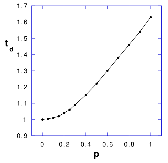
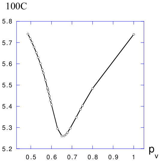
We have solved Eq. (60) numerically and the results for are shown in Fig. 1. The -dependence is indeed significant, becoming linear at high ; in the range we find . Thus (Eq. IV.1) at while at . We note also the significant enhancement in the value of in the latter case, i.e. . We note that the RG expansion is valid for , which limits Eq. (63) (by inserting it in Eq. (61)) to .
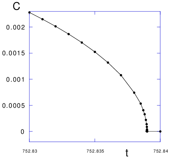
At we find that the variable first increases, then decreases, corresponding to weakening of the term, and finally increases up to at the scale where we should stop the renormalization process. The temperature dependence of is shown on Fig 2. We see that the correlation length as which shows that the phase transition is a continuous one. We note that the early estimate of Glazman and Koshelev glazman2 of the decoupling temperature gives a result similar to Eq. (63). They derive a condition for large fluctuations which by itself does not prove a phase transition; furthermore the estimated critical temperature vanishes with , i.e. it is incorrect at . The large fluctuation condition is close in spirit to the SCHA method and is further discussed in section V.
We present now numerical solutions of the full RG equations (53) with and given by Eq.(54) in Figs. 3, 4, for the same initial conditions as in Fig. 2 [, ] and , . We choose and these initial conditions since in this case the SCHA method (see section IV) yields a 1st order transition.
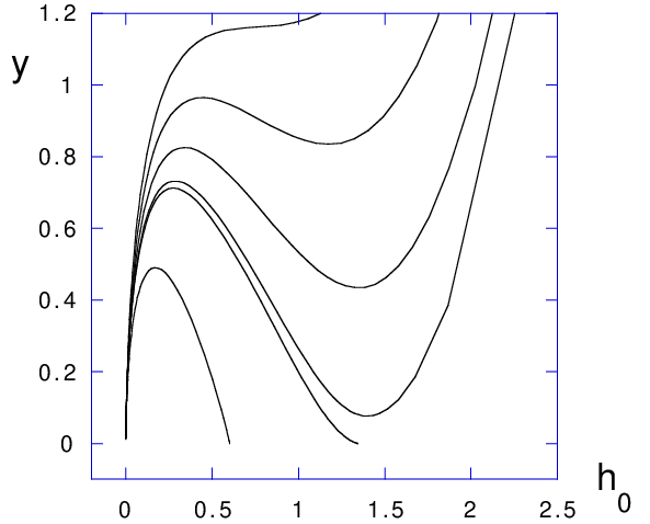
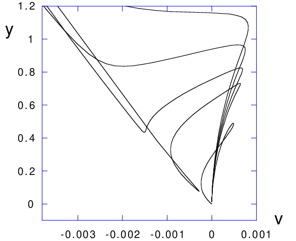
Figures 3 and 4 show the projected solution on the and planes, respectively. We find that ; for both the and variables vanish asymptotically, while at both and are relevant. The resulting correlation length diverges at , similar to Fig. 2, i.e. the transition is continuous. We have examined the transition also by varying the initial ; the correlation length was always found to diverge at defining a continuous type phase transition.
Another scenario for a 1st order transition is via changing the initial value of . Assuming a flow into strong renormalized the free energy is dominated by
| (64) |
The minimum at changes from to at large a negative , . This hints at a 1st order transition at some initial negative ; this is not the decoupling transition, but rather a transition within the coupled phase .
To emphasize the asymptotic forms we have integrated the RG equations up to and show in Fig. 5 the corresponding correlation length. For these parameters, the asymptotic v becomes negative above (with ). The curve in Fig. 5 is continuous at this since is dominated by in the asymptotic regime. One needs to further increase until the asymptotic and values become comparable. In fact at we observe a marked change in slope for in Fig. 5. The asymptotic form is found with decreasing from as increases, saturating at when . Therefore, a 1st order transition is possible within the coupled phase, associated with the relative strength of the renormalized and variables. The transition occurs when the initial is sufficiently negative.
V Plasma resonance
We show here the relation and then apply Eq. (34) to evaluate . In presence of a weak time dependent electric field in the direction perpendicular to the layers the Josephson relation imposes a time dependent addition to the Josephson phase. The kinetic energy has the form
| (65) |
where is a dielectric constant. Expanding the Josephson coupling yields to 2nd order (the 1st order term has ). This form neglects the possible time dependence of the Josephson term, e.g. dynamics of pancake vortices which are assumed to be slow on the scale of . In particular the ”phase slip” frequency was shown koshelev to be much smaller than . The plasma frequency is then
| (66) |
We proceed to evaluate from Eq. (34). Within 2nd order RG the contribution to the free energy h3 has the form of Eq. (30, i.e. with
| (67) |
We are mainly interested in where (see Fig. 4) so that we can use the truncated Eqs. (55). We use here the solution (81) for either or , written as
| (68) |
where and in general . The asymptotic form is so that identifies the transition temperature, e.g. in 1st order RG and (68) reduces to Eq. (50). Using and (68), Eq. (34) finally yields
| (69) |
where is assumed, corresponding to our requirement that is well below melting. In particular for the case , which is relevant for BSSCO shibauchi; matsuda, we have and
| (70) |
which can also be derived directly with (50); at high temperatures we obtain . note that Eq. (70) is reproduced by the high temperature expansion Eq. (40) up to a prefactor . While the latter expansion is in general deficient, for evaluating it is reasonable, as discussed below Eq. (41).
Our main result for the decoupled phase in systems is Eq. (70). In comparison, the melted phase where individual pancakes are uncorrelated has a correlation length of , so that is a plausible guess, hence from Eq. (35) we have ; this form with a prefactor of order 1 was confirmed by simulations koshelev. Hence in the decoupled phase is larger by a factor ; furthermore, since ( is B independent) in the melted phase while in the decoupled phase it is or not too close to decoupling. Thus the temperature dependence of can distinguish between decoupled and liquid phases.
VI The SCHA method
In this section we derive the decoupling transition within the variational SCHA method, reproducing the results of ref.daemen. In particular, this method results in a 1st order transition at large . We compare the method to that of 2nd order RG and show where the deficiency of SCHA originates.
The SCHA proceeds by searching for the optimal Gaussian Hamiltonian of the form
| (71) |
so that is determined by minimization of the variational free energy
where the averaging as well as correspond to . is then
| (72) |
where the term corresponds to and we have used . The last term in (72) is the Josephson term with,
| (73) |
This defines a parameter ; the renormalized Josephson coupling is then .
Minimizing Eq. (72) yields
| (74) |
Using the form (46) and the variable with , Eqs. (73,74) reduce to a self consistent equation for
| (75) |
This equation has exactly the same structure as that of Eq. (57) within 2nd order RG if the asymptotic form of RG variable is used. However the detailed behavior is significant and can affect the critical properties; in fact, and are non-monotonic.
We can perform the integration in Eq. (75), neglecting the type function as in Eq. (59) (i.e. replacing by ) leading to
| (76) |
where and is defined in Eq. (61).
If the transition is continuous then diverges near so that the effective Josephson coupling ; Eq. (76) then yields . The RG result shows instead a weak p dependence even at small as in Eq. (62) and Fig. 1.
At a 1st order transition is finite; anticipating a large , but , Eq.(76) can be written as:
| (77) |
The product is bounded by at , hence as temperature approaches from below increases up to but then jumps to in the decoupled phase, i.e. a 1st order transition. The critical temperature is then
| (78) |
This result is similar to that from RG, Eq. (63), except that the slope is somewhat different. The significant difference is that RG yields a continuous transition even at large .
At even larger p, where , , Eq. (76) yields
| (79) |
As above, is bounded by at , hence a 1st order transition at
| (80) |
The results for weak and Eq. (80) for strong are the results given in Ref. daemen. The intermediate range Eq. (78) is not mentioned there, though the plotted decoupling fields in their Fig. 1 are consistent with as from Eq. (78). Furthermore, Eq. (80) yields which is incompatible with the requirement that is well below .
It is interesting to note that the early estimate of Glazman and Koshelev glazman2 of the decoupling temperature gives a result similar to (78) or (63). Within this estimate the term in Eq. (23) is expanded and the condition of large fluctuations with yields . (This condition indicates decoupling, though by itself does not prove a phase transition.) The result is then the same as Eqs. (73,74) with , therefore it yields indeed a result close to that of Eq. (78).
Our main result in this section is to show the formal similarity between SCHA and 2nd order RG as well as an important difference, i.e. the mass term which is generated by RG is scale dependent. Both methods show significant enhancement of with increasing Josephson coupling, however the transition remains continuous in the RG solution.
VII Conclusions
In recent experiments on BSCCO khaykovich; fuchs the phase diagram has shown a number of low temperature phases. Most of these transitions are disorder driven by either bulk pinning or by surface barriers. In particular the possibility that the second peak transition is a disorder driven decoupling has been suggested h1; h2. The significant reduction of the Josephson plasma resonance at the second peak supports a decoupling scenario shibauchi; matsuda, however a conclusive signature for decoupling has not been shown so far.
The signature of decoupling is that translational order is maintained, though with softer tilt modulous, while superconducting order is lost, i.e. (Eq. 28) and the critical current in the direction vanish at . An additional signature is the power law decay of the Josephson correlation at . We find that the decoupling transition temperature is at low fileds ( of Eq. IV.1) while it changes to at higher fields () with significantly enhanced temperatures .
We have shown that RG can be used to evaluate and hence the Josephson plasma frequency. In particular for weak coupling , as in BSCCO, we find that , in contrast to a behavior in the melted phase. This temperature dependence can serve to identify a decoupled phase.
In the present work we assume that V-I defects are not generated. Hence superconductivity is lost only in the direction (i.e. ) while 2-dimensional superconductivity is maintained parallel to the layers. Our neglect of V-I defects is in fact not justified, since they are generated at a lower temperature in the system dodgson; ledou, i.e. at . The true transition is a 3-dimensional one in which both decoupling and the defect transition coalesce, similar to the scenario h3. The actual transition temperature is between and the defect transition. It can be estimated by the temperature at which the correlation lengths of the defects and become comparable. Thus e.g., if , the Josephson coupling is renormalized to strong coupling before the term feels the V-I defects. Since (where is the pancake vortex core energy; if local lattice relaxation is included olive then ) is exponentially large, and is close to unless is extremely small.
We expect for systems like BSCCO or YBCO that decoupling affects mostly superconductivity in the direction. The current-voltage relation parallel to the layers is expected then to be nonlinear h1, except at very low currents where the few V-I defects would eventually lead to a linear Ohmic behavior. Similarly, the power law for the Josephson correlation would eventually, beyond the V-I spacing decay exponentially.
In conclusion we have studied the meaning and critical properties of the decoupling transition. On the theory side, in our view this is one of the few transitions of vortex matter which is fully understood. It remains to be seen if experiment can also provide clear realizations for this type of transition.
Acknowledgements.
This research was supported by THE ISRAEL SCIENCE FOUNDATION founded by the Israel Academy of Sciences and Humanities. We thank A. Aharony, G. Zaránd and S. Teitel for useful and valuable comments.Appendix A Expansions for
We present in this appendix an analytic expansion for the decoupling temperature within the reduced set of Eq. (60) with . The results show a significant enhancement when the parameter in Eq. (61) is large.
We consider where flows to zero and reaches a finite asymptotic value , since the integration of in Eq. (60) is convergent. We assume that the integration of the equation is dominated by and will examine below the validity of this assumption.
Integrating in Eq.(60) with yields
| (81) |
We now substitute this solution into the equation (60) and solve for ,
| (82) | |||||
where is also included in and the important parameter is defined in Eq. (61). Since at large , defines the transition point.
We can now examine the consistency of replacing by in the equation. The condition that approaches relatively fast is that the dependent terms in Eq. (82) are small at , i.e. is small (but ), hence and are large. It seems plausible then that our approximation is valid at . Alternatively, if then it has anyway a weak effect on the RG, i.e. the present derivation is valid at .
Eq. (82) shows that converges to if . We now substitute in (82) and obtain a self consistent equation for , which for the variable becomes a cubic equation
| (83) |
This cubic equation has solutions only if the condition is satisfied, where
| (84) |
Therefore, correspond to and defines the temperature of the phase transition as given in Eqs. (62,63).
References
- (1) For a review see P. H. Kes, J. Phys. I (France) 6, 2327 (1996).
- (2) B. Khaykovich, E. Zeldov, D. Majer, T. W. Li, P. H. Kes and M. Konczykowski, Phys. Rev. Lett. 76, 2555 (1996); B. Khaykovich, M. Konczykowski, E. Zeldov, R. A. Doyle, D. Majer, P. H. Kes and T. W. Li, Phys. Rev.B, 56, R517 (1997).
- (3) D. T. Fuchs, E. Zeldov, T. Tamegai, S. Ooi, M. Rappaport and H. Shtrikman, Phys. Rev. Lett. 80, 4971 (1998).
- (4) K. Deligiannis, P. A. J. de Groot, M. Oussena, S. Pinfold, R. Langan, R. Gagnon and L. Taillefer, Phys. Rev. Lett. 79, 2121 (1997).
- (5) N. Avraham, B. Khaykovich, Y. Myasoedov, M. Rappaport, H. Shtrikman, D. E. Feldman, T. Tamegai. P. H. Kes, M. Li, M. Konczykowski, K. van der Beek and E. Zeldov, Nature 411, 451 (2001).
- (6) T. Shibauchi, T. Nakano, M. Sato, T. Kisu, N. Kameda, N. Okuda, S. Ooi, and T. Tamegai, Phys. Rev. Lett. 83, 1010 (1999).
- (7) M. B. Gaifullin, Y. Matsuda, N. Chikumoto, J. Shimoyama, and K. Kishio, Phys. Rev. Lett. 84, 2945 (2000).
- (8) L. I. Glazman and A. E. Koshelev, Physica (Amsterdam) 173 C, 180 (1991).
- (9) L. I. Glazman and A. E. Koshelev, Phys. Rev. B43, 2835 (1991).
- (10) L. L. Daemen, L. N. Bulaevskii, M. P. Maley and J. Y. Coulter, Phys. Rev. Lett. 70, 1167 (1993).
- (11) For a review on the theory of vortex matter see G. Blatter, M. V. Feigel’man, V. B. Geshkenbein, A. I. Larkin and V. M. Vinokur, Rev. Mod. Phys. 66, 1125 (1995).
- (12) A. E. Koshelev, Phys. Rev. Lett. 77, 3901 (1996).
- (13) Y. -H. Li and S. Teitel, Phys. Rev. B47, 359 (1993)
- (14) B. Horovitz and T. R. Goldin, Phys. Rev. Lett. 80, 1734 (1998).
- (15) M. J. W. Dodgson, V. B. Geshkenbein and G. Blatter, Phys. Rev. Lett. 83, 5358 (1999).
- (16) B. Horovitz and P. Le Doussal, Phys. Rev. Lett. 84, 5395 (2000); Phys. Rev. B 71, 134202 (2005).
- (17) B. Horovitz, Phys. Rev. B60, R9939 (1999).
- (18) B. Horovitz (following companion article).
- (19) A. Morozov, B. Horovitz and P. Le Doussal, Phys. Rev. B67, 140505(R) (2003)
- (20) W. E. Lawrence and S. Doniach, in Proceedings of the Twelfth International Conference on Low Temperature Physics (LT-12), Kyoto, 1970, edited by E. Kanda (Keigaku, Tokyo, 1971) p. 361.
- (21) M. J. W. Dodgson, A. E. Koshelev, V. B. Geshkenbein and G. Blatter, Phys. Rev. Lett. 84, 2698 (2000); H. Fanghor, A. E. Koshelev and M. J. W. Dodgson, Phys. Rev. B67, 174508 (2003).
- (22) B.Horovitz, Phys.Rev. B 47, 5947 (1993).
- (23) T. R. Goldin and B. Horovitz, Phys. Rev. B58, 9524 (1998).
- (24) E. Olive and E. H. Brandt, Phys. Rev. B57, 13861 (1998).