Electronic glasses

Starting from the full electronic Hamiltonian (fermions with interactions and disorder) is a near impossible task. In the crystal phase some simplifications can be made since the particles are now discernable by their position. This allows for a minimal phenomenological model to describe such a crystal [22, 23, 24, 21]: one assumes that the particles are characterized by an equilibrium position $R^{0}_{i}$ and a displacement $u_{i}$ relative to this equilibrium position. In order to define uniquely the displacement one should not have topological defects such as dislocations in the crystal. I will come back to this point in Sec. 5.2. From the original quantum problem one has to define the “particles” of the crystal. If the wavefunction is localized enough then one can indeed ignore the exchange between the various sites and thus define “particles” that have a size given by the extension of the wavefunction as indicated in Fig. 4.

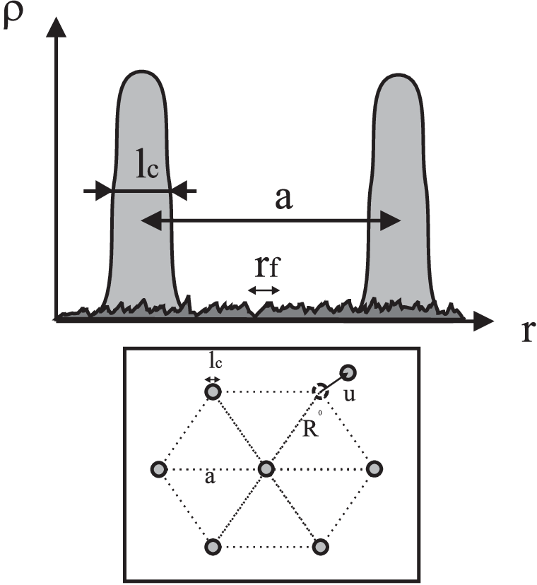
Of course the density fixes the lattice spacing $a$. These two lengthscales (size of particle, lattice spacing) are independent and should be kept. One then has to deal with the vibration modes of this crystal. As usual one considers the interaction between particles

$$H=\frac{1}{2}\sum_{i\neq j}V(R_{i}-R_{j})=\frac{1}{2}\int drdr^{\prime}V(r-r^{\prime})\rho(r)\rho(r^{\prime})$$

(1)

and expands to second order in the displacements. If the potential $V$ is short range this gives the standard elasticity. Here one has to be more careful since $V$ is the (long range) Coulomb interaction between the electrons. One has thus to distinguish the two modes presented in Fig. 5.

The compression mode changes the smeared density at one point of the crystal, creating an excess or a default charge. Such charges interact through the long range part of the Coulomb interaction. Since the density is essentially $\nabla u$ (I will be more precise later), this mode gives a contribution $V(q)q^{2}u^{*}_{q}u_{q}$ in the energy, where $V(q)$ is the Fourier transform of the Coulomb interaction. Since $V(r)\sim 1/r$, $V(q)\sim 1/q$ in two dimensions. The compression mode thus has an elasticity going as $|q|u^{*}_{q}u_{q}$. On the other hand the shear mode does not change the density (averaged over a couple of unit cells), and thus the long range part of the interaction does not couple to this mode. The coupling comes from the short range part (or if one prefers $V(q\sim 1/a)$). The shear mode has thus still an elasticity going as $q^{2}$. Being more precise one can define the longitudinal and transverse displacements for a mode $q$ by

$$\vec{u}(q)=\frac{\vec{q}}{q}u_{L}(q)+(\frac{\vec{q}}{q}\wedge\vec{z})u_{T}(q)$$

(2)

This leads to the action (see [24] for more details):

	$\displaystyle S$	$\displaystyle=$	$\displaystyle\frac{1}{2}\int_{\bf q}\frac{1}{\beta}\sum_{\omega_{n}}u_{L}(q,\omega_{n})(\rho_{m}\omega_{n}^{2}+c_{L}(q))u_{L}(-q,-\omega_{n})$		(3)
			$\displaystyle+u_{T}(q,\omega_{n})(\rho_{m}\omega_{n}^{2}+c_{T}(q))u_{T}(-q,-\omega_{n})$
			$\displaystyle+\rho_{m}\omega_{c}\omega_{n}[u_{L}(q,\omega_{n})u_{T}(-q,-\omega_{n})-u_{T}(q,\omega_{n})u_{L}(-q,-\omega_{n})]$

$\int_{\bf q}$ denote the integration over the Brillouin zone $\int_{BZ}\frac{d^{2}q}{(2\pi)^{2}}$ and the $\omega_{n}$ are the standard Matsubara frequencies. The $\omega_{n}^{2}$ terms are coming from the $P^{2}/2m$ term in the Hamiltonian, and are the ones embedding the quantum nature of the crystal. For a quantum crystal it is impossible to have the particles at rest since both its position and position would be determined simultaneously. Thus even at $T=0$ quantum fluctuations exists. The third term in (3) comes from the Lorentz force, that exists if the particles are submitted to a magnetic field. The action corresponding to this force is simply the work of the force $F_{L}\cdot u$ where $F_{L}=q\partial_{\tau}u\wedge B$. $\rho_{m}\simeq{m\over{\pi a^{2}}}$ is the mass density and $\omega_{c}=eB/m$ the cyclotron frequency.

The precise coefficients $C_{L,T}(q)$ are the elastic coefficients for the longitudinal and transverse modes respectively. These coefficients can be obtained from an expansion of the coulomb correlation energy of the WC in terms of the displacements [25, 26]. As I discussed $C_{L}(q)\sim|q|$ and $C_{T}(q)\sim q^{2}$. Keeping the lowest terms of the expansion one has

	$\displaystyle C_{L}(q)$	$\displaystyle=$	$\displaystyle d|q|-bq^{2}$
	$\displaystyle C_{T}(q)$	$\displaystyle=$	$\displaystyle cq^{2}$		(4)

where $c$,$d$,$b$ are positive constants.

For a pure system the consequences of the quadratic Hamiltonian (3) are easy to carry out. The eigenmodes of the system are obtained by doing the analytic continuation $i\omega_{n}\to\omega+i\delta$. In the absence of magnetic field the longitudinal and transverse modes are decoupled. The longitudinal one has a dispersion

$$\rho_{m}\omega^{2}_{L}=C_{L}(q)\sim d|q|$$

(5)

This is the standard plasmon dispersion in $d=2$. Because of the Coulomb repulsion it is extremely hard to excite this mode. The system is very rigid (much more than a normal elastic system) since it does not like to have its local density changed. This is not the case of the transverse mode which keeps a phonon-like dispersion

$$\rho_{m}\omega^{2}_{T}=C_{T}(q)\sim cq^{2}$$

(6)

In the presence of a large magnetic field the two modes are mixed. It is easy to obtain the new eigenmodes by diagonalizing the two by two matrix in (3). This gives the modes of Table 1.

The “plasmon” mode is now pushed to the cyclotron frequency $\omega_{c}$, while there is a low energy mode with a $q^{3/2}$ dispersion. This low energy mode is the mode that was probed in the sound absorption experiment shown in Fig. 2.

For the crystal, the current is simply given by $J=e\rho_{0}\partial_{t}u$, making thus the conductivity very simple to compute since it is essentially the correlator of the displacements (up to a factor $\omega^{2}$). The conductivity is thus given by

$$\sigma_{\alpha\beta}(\omega)=-(e\rho_{0})^{2}i(\omega+i\delta)\langle u_{\alpha}(q=0,\omega_{n})^{*}u_{\beta}(q=0,\omega_{n})\rangle_{i\omega_{n}\to\omega+i\delta}$$

(7)

In the absence of magnetic field the conductivity is simply

$$\sigma_{xx}(\omega)=\frac{e^{2}\rho_{0}}{m}\frac{i}{\omega+i\delta}$$

(8)

The real part is thus just a $\delta$-function at zero frequency. This traduces the fact that the crystal can slide freely in response to an external force (the electric field). The pure quantum crystal is thus a perfect conductor. In the presence of a finite magnetic field, the conductivity becomes

$$\sigma_{xx}(\omega)=\sigma_{yy}(\omega)=\frac{e^{2}\rho_{0}}{m}\frac{-i(\omega+i\delta)}{-(\omega+i\delta)^{2}+\omega_{c}^{2}}$$

(9)

Thus the $\delta$-function peak is pushed at the finite frequency $\omega_{c}$. The d.c. conductivity is zero. This is due to the fact that in presence of a magnetic field the electrons describe cyclotron orbits, and do not drift in response to a static electric field. Paradoxically the system is then an insulator. On the other hand the Hall conductivity is given by

$$\sigma_{xy}(\omega)=\frac{e^{2}\rho_{0}}{m}\frac{\omega_{c}}{-(\omega+i\delta)^{2}+\omega_{c}^{2}}$$

(10)

This gives for the Hall resistivity

$$\rho_{xy}(\omega)=\frac{\sigma_{xy}}{\sigma_{xx}^{2}+\sigma_{xy}^{2}}=\frac{m\omega_{c}}{e^{2}\rho_{0}}=\frac{B}{e\rho_{0}}$$

(11)

which quite remarkably is the classical Hall resistivity.

Of course these results are for the pure system only and the crucial question, in order to make contact with the experiments, is to determine how the disorder changes the above results.

The coupling of the crystal to the disorder writes

$$S_{\rm dis}=\int d\tau\int drV(r)\rho(r,\tau)$$

(12)

The potential $V$ represents the impurities. In these systems there are usually two main sources of disorder. One is provided by donors/acceptors far from the 2DEG. They interact with the 2DEG via the long range Coulomb interaction (see e.g. [27]). Since they are far from the 2DEG this produces a smooth potential. Another source of disorder is provided by interface roughness [28]. This type of disorder has a wavelength which is comparable or shorter than the lattice spacing of the crystal, and is most likely the main source of pinning.

In the limit where the impurities are weak and the pinning is collective, the disorder can be modelled by a gaussian potential, (see [22, 17] for a more in depth discussion of this limit)

$$\overline{V(r)V(r^{\prime})}=\Delta_{r_{f}}({r}-{r}^{\prime})$$

(13)

$\Delta_{r_{f}}$ is a delta-like function of range $r_{f}$ which is the characteristic correlation length of the disorder potential (see Figure 4). The density reads

$$\rho(r)=\sum_{i}\overline{\delta}(r-R^{0}_{i}-u_{i})$$

(14)

where $\overline{\delta}$ is a $\delta$-like function of range $l_{c}$ (see Figure 4) and $u_{i}\equiv u(R^{0}_{i})$. Since the disorder can vary at a lengthscale $r_{f}$ a priori shorter or comparable to the lattice spacing $a$, the continuum limit $u_{i}\to u(r)$, valid in the elastic limit $|u_{i}-u_{i+1}|\ll a$ should be taken with care in the disorder term. This can be done using the decomposition of the density in terms of its Fourier components [29, 30]

$$\rho(r)\simeq\rho_{0}-\rho_{0}\nabla\cdot{u}+\rho_{0}\sum_{{K}\neq 0}e^{i{K}\cdot({r}-{u}(r))}$$

(15)

where $\rho_{0}$ is the average density and $K$ are the reciprocal lattice vectors of the perfect crystal. This is a decomposition of the density in Fourier harmonics determined by the periodicity of the underlying perfect crystal as shown on Fig. 6.

Let me examine the various terms. The first term is just the average density. The second one is the textbook expression of the density in terms of the displacements. It corresponds to a density averaged at a scale of a few lattice spacing (smeared density). This part of the density thus traduces local changes of the density due to compression modes similar to the ones in Fig. 5. The other terms describes change of the density at a lengthscale comparable or smaller than the lattice spacing. The sum over the reciprocal lattice vectors $K$ obviously reproduces the $\delta$ function peaks of the density (14). The finite range of $\overline{\delta}$ is recovered [30] by restricting the sum over $K$ to momentum of order $K_{\rm max}\sim\pi/l_{c}$. This expression of the density is quite useful since it allows to express the density at all scales in term of the slowly varying function $u(r)$. The price to pay is the more complicated form of the operator that embeds in its very form the information about the periodicity of the crystal and the size of the particles. This is a quite useful trick, initially introduced for Luttinger liquids [31]. One keeps only the low energy-long wavelength part of the displacement field, since this field has a well defined continuum limit, and thus a quite simple continuum Hamiltonian (elastic Hamiltonian in this case). But it is still possible using this field that varies at a lengthscale large compared to the lattice spacing (this is the essence of the elastic limit) to describe phenomena that vary at a much shorter lengthscale, provided that one uses the proper form for the operator in terms of this continuum field. This expression of the density allows to write quite simply the coupling to disorder. Using the representation of density (15) it is easy to show [22, 20] that a Luttinger liquid is indeed very similar to the quantum crystals that are described here.

Using the expression of the density (15) one sees that different Fourier component of the disorder play different roles. The Fourier components close to $q\sim 0$ couple to $\nabla u$. These terms play little role (see [20] for more details). In our case because the compression modes are quite stiff thanks to the Coulomb repulsion this is even more so. The main effect of the disorder comes from the other Fourier modes, i.e. the ones that are close to $q\sim K$ where $K$ is one of the vectors of reciprocal lattice of the crystal. The effect of the disorder can thus be written as

$$S_{\rm dis}\simeq\sum_{K\neq 0}\int drV(r)\rho_{0}e^{iK(r-u(r))}$$

(16)

The coupling to the displacements is highly nonlinear which of course makes this problem very difficult to solve. The action (12) and (3) is the minimal model needed to describe a disordered quantum crystal.

For a quantum problem, the disorder is time independent. Thus if one looks at the space-time trajectories of the particles, as shown in Fig. 7, one can view the system as a classical system of lines in $d+1$ dimensions [22, 20]. These lines are pinned by columnar defects, i.e. defects independent of one of the coordinates ($\tau$ in this case).

The problem of lines pinned by columnar defects has been studied extensively in the context of vortex lattices [32, 33], where in that case the defects are produced by heavy ions irradiation. Thus some features of the two systems are indeed similar and one can gain considerable insight by thinking in term of the classical system of lines. There is however an important difference. In the classical system $\tau$ is simply one spatial direction, one is thus looking at the static of such systems. The dynamics of classical systems is a different problem, where an additional time $t$ needs to be introduced (see e.g. [17, 34]). For the quantum problem, $\tau$ is the imaginary time of the problem. Thus $\tau$ dependence of the quantities is describing the equilibrium dynamics of the quantum problem. In order to get the proper quantum dynamics however one should make the analytical continuation $\tau\to it$ (or more precisely $i\omega_{n}\to\omega+i\delta$). This analytical continuation, although seemingly innocent has severe consequences and changes many behaviors. Though although some analogy between the static (but $z=\tau$ dependent quantities such as e.g. the tilt of the lines) behavior of classical crystals with columnar defects and the dynamics behavior of quantum crystals can be made, one should exert great care because of the analytic continuation needed for the quantum problems, which ultimately leads to some differences in physics.

In order to define the basic properties of such systems let me consider first what happens in the ground state of the problem. Since the disorder is time independent, one can consider all displacements as time independent to get the ground state (it corresponds to the mode $\omega_{n}=0$). The problem is thus equivalent to a classical system in $d$ dimensions. The time integration is just providing a factor $\beta$ in front of the action and the problem is equivalent to determine the partition function of a systems

$$Z=\int{\mathcal{D}}u[r]e^{-\beta H_{cl}}$$

(17)

where

$$H_{\rm cl}=\frac{c}{2}\int d^{d}r(\nabla u)^{2}+\rho_{0}\int V(r)\rho(r)$$

(18)

I have forgotten for simplicity in the above formula the difference between longitudinal and transverse modes and simply rewritten everything with a standard elasticity (this corresponds in fact to the transverse mode with an elastic constant $C_{T}(q)\sim q^{2}$). It is thus enough to examine a classical crystal, in presence of point like defects (for more details see [17, 34]).

In order to understand the basic physics of such problem a simple (but ground breaking !) scaling argument was put forward by Larkin [35]. To know whether the disorder is relevant and destroys the perfect crystalline order, let me assume that there exists a characteristic lengthscale $R_{a}$ for which the relative displacements are of the order of the lattice spacing $u(R_{a})-u(0)\sim a$. If the displacements vary of order $a$ over the lengthscale $R_{a}$ the cost in elastic energy from (18) is

$$\frac{c}{2}R_{a}^{d-2}a^{2}$$

(19)

by simple scaling analysis. Thus in the absence of disorder minimizing the energy would lead to $R_{a}=\infty$ and thus to a perfect crystal. In presence of the disorder the fact that displacements can adjust to take advantage of the pinning center on a volume of size $R_{a}^{d}$ allow to gain some energy. Since $V$ is random the energy gained by adapting to the random potential is the square root of the potential over the volume $R_{a}^{d}$, thus one gains an energy from (18)

$$-VR_{a}^{d/2}\rho_{0}$$

(20)

Thus minimizing (19) plus (20) shows that below four dimensions the disorder is always relevant and leads to a finite lengthscale

$$R_{a}\sim a\left(\frac{c^{2}a^{d}}{V^{2}\rho_{0}^{2}}\right)^{1/(4-d)}$$

(21)

at which the displacements are of order $a$. The conclusion is thus that even an arbitrarily weak disorder destroys the perfect positional order below four spatial dimensions, and thus no disordered crystal can exist for $d\leq 4$. This is an astonishing result, which has been rediscovered in other context (for charge density waves $R_{a}$ is known as Fukuyama-Lee [36] length and for random field Ising model this is the Imry-Ma length [37]). Of course it immediately prompt the question of what is the resulting phase of elastic system plus disorder?

Since solving the full problem is tough another important step was made by Larkin [35, 38]. For small displacements he realized that (18) could be expanded in powers of $u$ leading to the simpler disorder term

$$H_{\rm larkin}=\int d^{d}rf(r)u(r)$$

(22)

where $f(r)$ is some random force acting on the vortices. Because the coupling to disorder is now linear in the displacements the Larkin Hamiltonian is exactly solvable. Taking a local random force $\overline{f(r)f(r^{\prime})}=\Delta\delta(r-r^{\prime})$ gives for the relative displacements correlation function and structure factor

$\displaystyle B(r)=\overline{\langle[u(r)-u(0)]\rangle}$

$\displaystyle=$

$\displaystyle B_{\rm thermal}(r)+\frac{\Delta}{c^{2}}r^{4-d}$

(23)

where $\langle\rangle$ denotes the thermodynamics average and $\overline{\cdots}$ denotes the disorder average. $B_{\rm thermal}$ is the same correlation function in the absence of disorder due to thermal fluctuations (which remain bounded in $d>2$ and are thus negligeable at large distance compared to the disorder term). Thus the solution of the Larkin model confirms the scaling analysis: (i) displacements do grow unboundedly and thus perfect positional of the crystal is lost; (ii) the lengthscale at which the displacements are of the order of the lattice is the similar to the one given by the scaling analysis. In addition the Larkin model tells us how fast the positional order is destroyed: the displacements grow as power law thus one can expect the positional order to be destroyed exponentially fast. However these two conclusions should be taken with a serious grain of salt. Indeed the Larkin model is an expansion in powers of $u$, and thus cannot be valid at large distance (since the displacements grow unboundedly the expansion has to break down at some lengthscale). What is this characteristic lengthscale? A naive expectation is that the Larkin model cease to be valid when the displacements are of order $a$ i.e. at $r=R_{a}$. In fact this is too naive as was understood by Larkin and Ovchinikov. To understand why, in a transparent way, let me use the expression for the density (15) This immediately allows to reproduce the Larkin model by expanding the disorder term (18)

$$\rho_{0}\int d^{d}r\sum_{K}e^{iK(r-u(r))}V(r)$$

(24)

in powers of $u$. Clearly the expansion is valid as long as $K_{max}u\ll 1$ This will thus be valid up to a lengthscale $R_{c}$ such that $u(R_{c})$ is of the order of the size of the particles $l_{c}$. Note that this lengthscale is different (and quite generally smaller) than the lengthscale $R_{a}$ at which the displacements are of the order of the lattice spacing $a$. The Larkin model cease to be valid way before the displacements become of the order of $a$ and thus cannot be used to deduce the behavior of the positional order at large length scale. In addition it is easy to check that because the coupling to disorder is linear in the Larkin model, this model does not exhibit any pinning, since the model is invariant by changing $u(r)\to u(r)+C$ where $C$ is an arbitrary constant (remember that the total of the random forces has to be zero $\int drf(r)=0$). Thus sliding by an arbitrary amount does not cost any energy and any addition of an external force leads to a sliding of the vortex lattice. Thus the lengthscale at which this model breaks down is precisely the lengthscale at which pinning appears [38]. The lengthscale $R_{c}$ is thus the lengthscale above which various chunks of the system are collectively pinned by the disorder. A simple scaling analysis on the energy gained when putting an external force

$$H=\int d^{d}rF_{\rm ext}u(r)$$

(25)

allows to determine the critical force needed to unpin the lattice. Assuming that the critical force needed to unpin the lattice is when the energy gained by moving due to the external force is equal to the balance of elastic energy and disorder $\frac{c}{2}l_{c}^{2}R_{c}^{d-2}$, one obtains for the critical force needed to move the lattice

$$F_{c}\propto\frac{cl_{c}}{R_{c}^{2}}$$

(26)

This is the famous Larkin-Ovchinnikov relation which allows to relate a dynamical quantity (the critical force at $T=0$ needed to unpin the lattice) to purely static lengthscales, here the Larkin-Ovchinikov length at which the displacements are of the order of the size of the particle. Let me insist again that this lengthscale controlling pinning is quite different from the one $R_{a}$ at which displacements are of the order of the lattice spacing at that controls the properties of the positional order.

These two lengthscales $R_{c}$ and $R_{a}$ are thus the crucial ones in controlling the properties of a pinned classical crystal, and thus will of course be crucial for our quantum crystals. For the quantum crystals this leaves us with two main questions: (i) what is the conductivity of the system, and which length controls it; (ii) what happens beyond the length $R_{a}$.

Up to know we have been on relatively firm ground, but answering the above questions, even for a classical crystal is a tough cookie. Given the difficulty in obtaining the answers, instead of a solution people have been happy for a long time with a kind of consensus on how the system “should” behave, based on physical intuition and some incomplete, or in some cases incorrect proofs. I will give in this section a summary of these preconceived ideas on disordered crystals, since they were at the root of most of the physical solutions given for the dynamics. Fortunately recent progress have made it possible to truly analyze these systems. As usual the true behavior turned out to be quite different from what was naively believed. I will examine these solutions in the next section. But for the moment let me go along and describe the (incorrect) picture of a disordered crystal, that was used for a long time.

The first point is to naturally assume that because there exists a lengthscale $R_{a}$ for which displacements are of the order of the lattice spacing, positional order is destroyed exponentially fast beyond this lengthscale. This behavior would be in agreement with the too naive extrapolation of the Larkin model to arbitrary lengthscales and is in agreement with exact solutions of interface problems in random environments (so called random manifold problems) and solutions in one spatial dimension. It was thus quite naturally assumed that an algebraic growth of displacements was the correct physical solution of the problem, and thus that the positional order would be destroyed exponentially beyond the length $R_{a}$. This led to an image of the disordered vortex lattice that consisted of a crystal “broken” into crystallites of size $R_{a}$ due to disorder. To reinforce this image (incorrect) “proofs” were given [39] to show that due to disorder dislocations would be generated at the lengthscale $R_{a}$ (even at $T=0$) further breaking the crystal apart and leaving no hope of keeping positional order beyond $R_{a}$. A summary of this (incorrect) physical image is shown on Fig. 8.

If one assumes that all positional order is lost, this allows to solve for the dynamics of the problem. In that case one can consider that each crystallite is pinned independently. When one tries to move it it sees a pinning potential that one can approximate by an harmonic well. The shape of the well depends on the size of the crystallite. If the system is submitted to an electric field at frequency $\omega$, each crystallite will respond as a particle in a well. Crudely speaking the minimal frequency one can excite is (using $\omega=cq$ and $q_{\rm min}\sim 1/R_{a}$) is

$$\omega_{\rm pin}\propto\frac{c}{R_{a}}$$

(27)

The perfect conductivity of the pure crystal, i.e. the $\delta$-function peak that existed at zero frequency is now pushed to the finite frequency $\omega_{\rm pin}$, as shown in Fig. 9.

If there is a finite magnetic field the peak at $\omega_{c}$ is essentially unchanged and there is a second peak that appears at $\omega_{\rm pin}$. Of course the approximation of independent crystallites is not exactly true and the coupling between the crystallites as well as the distribution of pinning strength leads to a broadening of the peaks. The broadening is hard to determine precisely since one does not know exactly the static solution, so quite often a lorentzian broadening is assumed. This physical image inspired from pioneering theories [36] used for charge density waves allows to compute, using some approximations, the optical conductivity (see e.g. [20] for further details on that point). This gives specific predictions, in particular the density dependence of the pinning frequency would be from the above mentioned approximations $\omega_{p}\propto n^{1/2}$.

Measuring the optical conductivity is thus a very powerful way to check for the presence of a pinned Wigner crystal. An example of data is shown in Fig. 10.

One clearly observes a pinning peak in the optical conductivity. However there are many problems. First the broadening is far from being simply lorentzian as is obvious when simply looking at the data. A much more serious problem comes from the density dependence of the pinning frequency that can be extracted from the above data and is shown in Fig. 11.

When one compares the experiments, with these theoretical predictions the agreement is qualitatively wrong. The predicted result would be totally opposite to the data which shows a decrease of the pinning frequency with the density. Such important problems when one tries to compare with the data could cast serious doubts on the interpretation of the insulating phase in terms of a Wigner crystal and quite naturally other interpretations for this phase have been proposed [41].

In fact, the reason of this discrepancy is that the phenomenological image of nearly independent crystallites is simply plain wrong. In order to be able to compute the transport properties we thus need sharper tools to solve the problem of pinned quantum crystals. These are the tools I now present.

The first method is to try to reduce this problem to the “best” quadratic problem approximating $S_{\rm el}+S_{\rm dis}$. The most brutal way would be to simply expand the cosine, but as is well known for sine-Gordon problems this is very often a poor approximation. Here is would be a complete catastrophe for reasons that will become clear later. An improved way is to perform a self consistent calculation. The simplest way to implement such a scheme it through Feynman’s variational approach [44]. The method has been extended to deal with replicas in [45]. Let me define a trial action $S_{0}$. Then the free energy $F$ of the system verifies

$$F\leq S_{\rm var}=F_{0}+\langle S-S_{0}\rangle_{0}$$

(41)

where $\langle\rangle_{0}$ denotes an average taken with the action $S_{0}$. If $S_{0}$ depends on some variational parameter one can hope that the “best” way (i.e. the one giving a physics as close as possible to the one of the true action $S$) of choosing this parameter is to minimize $S_{\rm var}$. Let us take for $S_{0}$ the most general quadratic action

$$S_{0}=\frac{1}{\beta\Omega}\sum_{ab}\sum_{q,\omega_{n}}G^{-1}_{ab}(q,\omega_{n})u_{a}^{*}(q,\omega_{n})u_{b}(q,\omega_{n})$$

(42)

The choice of a quadratic action for $S_{0}$ has two motivations: (i) quadratic actions are the only ones with which one is able to compute something; (ii) on a physical basis one can expect the properties of the system to be dominated by the small oscillations around one of the minima of the cosine. We will have to come back to this assumption. In doing so one implicitly neglects excitations that can take the system from one minimum of the cosine to the other. For the sine-Gordon model these excitations are known as solitons [46]. For the pure problem this method is equivalent to the well known self consistent harmonic approximation, and gives excellent results. The disordered case is more involved [22, 20]. In particular special case should be paid to the mode $\omega_{n}=0$ since the disorder is time independent. I will only sketch the main lines here. The full Green’s functions are here the variational parameters. They are determined by

$$\frac{\partial S_{\rm var}}{\partial G_{ab}(q,\omega_{n})}=0$$

(43)

Using (41) leads to nasty integral equations, roughly of the form

$$G^{-1}_{ab}(q,\omega_{n})=(\omega_{n}^{2}+q^{2})\delta_{ab}+\int d\tau[1-\cos(\omega_{n}\tau)]e^{-\frac{1}{\beta\Omega}\sum_{q,\nu_{n}}G_{ab}(q,\nu_{n})\cos(\nu_{n}\tau)}\ldots$$

(44)

One has to remember that the limit $n\to 0$ should be taken at the end so $G_{ab}$ is in fact a $0\times 0$ matrix. In order to invert this matrix to solve the equations (44) one needs to know what is the structure of such matrices. In the original action, $S_{\rm el}$ is purely diagonal in replicas, whereas $S_{\rm dis}$ couples each replica with another and is thus independent of the value of the indices $a,b$. This suggests that a good structure for $G_{ab}$ is to take one (for each value of $q$ and $\omega_{n}$ of course) value on the diagonal, and one unique value away from the diagonal

$$G_{ab}=[\tilde{G}-G]\delta_{ab}+G$$

(45)

Such a matrix structure is shown in Fig. 12.

This is the natural choice, and is called replica symmetric since it respects the permutation symmetry between the replicas. The matrix depends in fact on only two numbers: the value on the diagonal $\tilde{G}$ and the off diagonal value $G$. It is easy to see that such matrices can be inverted and have a well defined limit when $n\to 0$. Calling $\tilde{G}^{-1}$ and $G^{-1}$ the diagonal and off diagonal value of the matrix $G^{-1}_{ab}$ and the connected part $G_{c}=\sum_{b}G_{ab}$ one has the inversion formulas (in the limit $n\to 0$)

$$G_{c}=\frac{1}{G_{c}^{-1}}\quad,\quad G=-\frac{G^{-1}}{(G_{c}^{-1})^{2}}$$

(46)

This allows to close the integral equations (44) and in principle to solve them. Unfortunately, it is easy to see that (45) cannot be right. This can be seen if one brutally expand the cosine. This indeed corresponds to a RS structure and gives “directly” $S_{0}$ (this approximation corresponds to the variational approach if one assumes the RS structure and that the disorder $\Delta$ is large). In that case only the $\omega_{n}=0$ frequency appears due to the double integration on $\tau$ and $\tau^{\prime}$. Since the action is quadratic this means that the disorder would only affect the mode $\omega_{n}=0$, and thus would be unable to change the current. This is obviously completely opposite to the idea of pinning, so such an approximation misses all this physics. The answer to this paradox resides in the assumption of the replica symmetric structure for the matrix $G_{ab}$. Indeed as is now well known for spin glasses, such a saddle point might be unstable [47]. In that case one should look for another structure for $0\times 0$ matrices. This structure was discovered by Parisi, and breaks the replica symmetry [48]. The matrix is now a hierarchical matrix. There is not a single element off diagonal but many values defined in a hierarchical way. I will not enter in the structure of the theory, and refer the reader to [49, 20] for a discussion. A pictorial representation of the matrix is shown in Fig. 12. Such matrices can also be inverted in the $n\to 0$ limit. This structure is called replica symmetry breaking. In this limit the off diagonal element becomes a function $G(v)$ of a continuous variable varying between zero and one. If $G(v)$ is a continuous function one speaks of continuous RSB, whereas if $G(v)$ has step(s) one talks about $n$-step RSB ($n$ being the number of steps). I will not dwell too much on the physical interpretation and refer the reader to [20]. As is well known for spin glasses, the occurrence of RSB signals glassiness, and the presence of metastable states. Since there is one matrix $G_{ab}(q,\omega_{n})$ for each value of $q$ and $\omega_{n}$, the replica structure depends a priori on $q$ and $\omega_{n}$. For quantum problems since the disorder is time independent one can show [22] that one has off diagonal replica terms only for the mode $\omega_{n}=0$. The structure is replica symmetric for $q>1/R_{c}$ and RSB for $q<1/R_{c}$. This confirms the physical picture that pinning and metastability appear above the Larkin length $R_{c}$.

RSB might look like magic¹¹ 1 This is metaphysical question, since the only point is whether a method works or not!, so let us try to solve our disordered problem by a more conventional renormalization approach. Doing it on quantum problems is tedious so I will explain the method on a classical system. One simply takes $\hbar=0$ in the quantum action which removes all time dependence in time of $u(r,\tau)$. The system is thus described by the classical action

$\displaystyle S$

$\displaystyle=$

$\displaystyle\frac{c}{2T}\sum_{a}\int d^{d}r(\nabla u_{a}(r))^{2}-\frac{\Delta}{T^{2}}\sum_{ab}\int d^{d}r\cos(K(u_{a}(r)-u_{b}(r)))$

(47)

where I have retained only a single harmonic in the disorder term for simplicity. To implement an RG procedure one would decompose $u_{a}(r)$ into fast and slow modes. If for example $\Lambda$ is a cutoff in $q$ space and $\Lambda^{\prime}$ a smaller cutoff, one defines ($\Omega$ is the volume of the system)

	$\displaystyle u_{a}(r)$	$\displaystyle=$	$\displaystyle u_{a}^{<}(r)+u_{a}^{>}(r)$		(48)
		$\displaystyle=$	$\displaystyle\frac{1}{\Omega}\sum_{q<\Lambda^{\prime}}u_{a}(q)e^{iqr}+\frac{1}{\Omega}\sum_{\Lambda^{\prime}<q<\Lambda}u_{a}(q)e^{iqr}$

One then integrates over the fast modes ($\Lambda^{\prime}<q<\Lambda$) to get an effective action with new coupling constants for the slow modes. Since the cutoff has changed it is then convenient to rescale space by $q=q^{\prime}\Lambda^{\prime}/\Lambda$ or $r=r^{\prime}\Lambda/\Lambda^{\prime}$, such that the new space variable $q^{\prime}$ has again a cutoff $\Lambda$. One can then iterate this procedure. Even without performing the integration over the fast modes let me look at the bare dimensions of the operators (tree level). Let us assume that $u$ scales as $u\sim L^{\zeta}$. One sees directly that periodic systems are peculiar. Because the disorder term is a cosine, with a periodicity which corresponds to the lattice spacing, this periodicity cannot be changed in the renormalization. This imposes $\zeta=0$ [29, 30]. Let me parametrize the cutoff by $\Lambda(l)=\Lambda_{0}e^{-l}$, where $\Lambda_{0}$ is the initial cutoff. In order to keep the elastic part of the action invariant, one should thus have

$$\frac{1}{T(l+dl)}=\frac{1}{T(l)}\left(\frac{\Lambda(l)}{\Lambda(l+dl)}\right)^{d-2}$$

(49)

the $d-2$ comes from the integration $d^{d}r$ and the $\nabla^{2}$. This gives the scaling dimension for the temperature

$$\frac{dT(l)}{dl}=T(l)(2-d)$$

(50)

We thus see that for $d>2$ the temperature scales to zero. This is in agreement with the fact that the competition between disorder and elasticity is an energy problem, where the temperature plays little role. Let us look at the renormalization of the disorder term. Performing the same rescaling of $d^{d}r$ and using (49) for the temperature gives

$$\Delta(l+dl)=\Delta(l)\left(\frac{\Lambda(l+dl)}{\Lambda(l)}\right)^{d-4}$$

(51)

giving the equation

$$\frac{d\Delta(l)}{dl}=\Delta(l)(4-d)$$

(52)

We thus see that the disorder is relevant below $d=4$. Note that around $d=4$ the temperature is indeed irrelevant. One could thus naively think that this problem is quite similar to the standard $4-\epsilon$ renormalization in critical phenomena. There is however an important difference. Let us compare the present problem with a standard (non disordered problem) in the standard $\phi^{4}$ theory. Let me denote the action for this problem

$$\frac{c}{2T}\int d^{d}r(\nabla\phi)^{2}+\frac{\lambda}{T}\int d^{d}r\phi^{4}+\frac{\mu}{T}\int d^{d}r\phi^{6}$$

(53)

In that case and contrarily to the disorder case both the elastic term and the “potential” terms have the same power of the temperature. This is of course the signature that a normal phase transition results from a competition energy-entropy. The extra factor of $1/T$ in front of the cosine in (47) is the way for the replicated action to indicate that before averaging one had to compare the two energies of the elastic term and of the disorder term. For (53) one absorbs the factor $e^{-(d-2)dl}$ coming from the spatial rescaling in the rescaling of $u$ and one leaves the temperature invariant. This traduces the fact that a problem at $T=T_{c}$ stays at $T_{c}$. The rescaling for $u$ thus becomes

$$\phi^{2}(l+dl)=\phi^{2}(l)e^{(d-2)dl}$$

(54)

This gives for the renormalization of the coupling constants

	$\displaystyle\frac{d\lambda}{dl}$	$\displaystyle=$	$\displaystyle\lambda(4-d)$
	$\displaystyle\frac{d\mu}{dl}$	$\displaystyle=$	$\displaystyle\mu(6-2d)$		(55)

Thus all terms in the potential that have high (i.e. larger than $4$) powers of $u$ are irrelevant. Thus regardless of the precise form of the potential, one can always expand in power series and the only important term is the $\phi^{4}$ term. The situation is totally different for the disordered system [50]. In that case $u$ does not scale. It means that all terms in a power series expansion of the potential have the same scaling dimension and are equally relevant around four dimensions. Thus instead of having a single RG equation for a single parameter $\lambda$ one has now an infinity of (a priori coupled) RG equations for all the coefficients of the terms in the power series expansion of the potential. In other words for the disorder problem one has now to renormalize the whole function corresponding to the potential term. This means that one has to start with a potential term

$$S_{\rm dis}=-\frac{1}{T^{2}}\sum_{ab}\int d^{d}r\Delta(u_{a}(r)-u_{b}(r))$$

(56)

where $\Delta(z)$ is a function whose initial ($l=0$) value is $\Delta_{l=0}(z)=\cos(Kz)$ but which will change form in the course of the renormalization. Because one has to keep the whole function under renormalization this procedure is known as functional renormalization group. I will not derive the equations to the next order (a good description of the derivation can be found in an appendix of [51]) but just give the result (for a classical crystal) [29, 30]

$$\frac{d\Delta(z)}{dl}=\epsilon\Delta(z)+\frac{1}{2}\Delta^{\prime\prime}(z)^{2}-\Delta^{\prime\prime}(z=0)\Delta^{\prime\prime}(z)$$

(57)

Needless to say this is much more complicated to solve than if one had a single parameter. But in addition there is an important feature of the solution. Because we eliminate modes $u_{a}$ becomes smoother and smoother thus in a sense $u_{a}-u_{b}$ becomes smaller and smaller under renormalization. Thus if the function $\Delta$ stayed analytic one could expand it in powers of $u$ to get

$$\Delta(u_{a}-u_{b})=\Delta(0)+\frac{1}{2}\Delta^{\prime\prime}(0)(u_{a}-u_{b})^{2}+\frac{1}{4!}\Delta^{(4)}(0)(u_{a}-u_{b})^{4}+\ldots$$

(58)

and one would be asymptotically dominated by the $(u_{a}-u_{b})^{2}$ term. This would give back a RS solution, and in fact exactly Larkin’s result. Since we know that this is incorrect beyond a certain lengthscale, something has to go wrong with the above expansion. The only way to escape this is if $\Delta^{(4)}(0)$ becomes very large (in fact infinite) so that the above expansion breaks down and that higher power continue to play a role. Thus to get the glassy physics the function $\Delta(z)$ should become nonanalytic beyond a certain lengthscale. One can check that this is indeed the case. The equation for $\Delta^{(4)}(0)$ is from (57)

$$\frac{d\Delta^{(4)}(0)}{dl}=\epsilon\Delta^{(4)}(0)+3[\Delta^{(4)}(0)]^{2}$$

(59)

which indeed explodes at the lengthscale

$$e^{l}=\left(\frac{\epsilon}{3\Delta_{0}}\right)^{1/\epsilon}$$

(60)

This corresponds indeed to the Larkin scale (compare with (21)). Beyond this lengthscale, although the function itself remains finite, it develop a non-analyticity. If one looks at the second derivative of $\Delta$ it develops a cusp, as shown on Fig. 13.

I will stop there on the FRG method since this would take us way beyond the level of these notes. For more on the FRG and further references see [49, 34, 52, 53]

Let me now examine what are the results for the disordered Wigner crystal. I will not reproduce the calculations here that can be found in [22, 20] for quantum crystals in general and in [23, 24] for the specific case of the Wigner crystal.

Using the variational method on (3) and (12) one finds that the most stable solution is an RSB one. This is suggestive that the pinned system indeed has glassy properties due to the pinning. I will thus use loosely the term Wigner glass in the following. Second, since we know have from the displacement-displacement propagator, one can compute the conductivity. An example of the results is shown in Fig. 14.

At first sight the agreement with the experimental data is much better (see [24] for a full discussion). Note that the broadening is non lorentzian in agreement with the data. More importantly one finds a decrease of the pinning frequency with the density as $\omega_{p}\propto n^{-3/2}$, as well as a good magnetic field dependence of the pinning frequency. This very good agreement gives a good confirmation that the insulating phase in the 2DEG under strong magnetic field is indeed a Wigner crystal collectively pinned by impurities.

What is the reason of this difference with the naive answers explained in Sec. 3.2? An inspection of the variational solution [23, 24] shows that in the full solution the pinning frequency is not controlled by $R_{a}$ as in the naive answer but by $R_{c}$ (in fact the formula is more complicated). This is a very satisfactory and physical result. Indeed as we discussed, for a classical crystal $R_{c}$ is the length that controls the pinning force. Although is it of course impossible to directly extrapolate it is quite reasonable to obtain that the pinning frequency, that is another manifestation of pinning, is also controlled by this lengthscale. This difference is crucial since, as in the Wigner crystal $l_{c}$ and $a$ are quite different $R_{c}$ and $R_{a}$ corresponds to quite different lengthscales and have in general quite different dependence in the various parameters. Since $R_{c}$ depends on the size of the particle $l_{c}$, this gives, for example for the case of strong magnetic field for which $l_{c}$ is just the cyclotron orbit, additional magnetic field dependence to the pinning frequency. This is to be contrasted with charge density waves for which $l_{c}\sim a$ due to the nearly sinusoidal density modulation and thus $R_{c}\sim R_{a}$. Thus borrowing directly the solutions that have been developed [36] for this case is dangerous and gives part of the physics incorrectly.

I refer the reader to [23, 24], for other physical properties such as the Hall conductivity. I will just mention here the compressibility. Defining the compressibility for a charged system is a delicate question since one has to maintain the neutrality of the system. Naively one relates the compressibility to the density-density correlation function by

$$\kappa=\lim_{q\to 0}\langle\rho(q,\omega_{n}=0)\rho(-q,\omega_{n}=0)\rangle$$

(61)

Let me look first at the pure system. The compressibility is simply (only the longitudinal mode plays a role)

$$\kappa(q)=\lim_{q\to 0}\frac{q^{2}}{c_{L}(q)}$$

(62)

If only short range interactions are present in the system the longitudinal mode is a phonon-like mode $c_{L}(q)\propto q^{2}$ and the one recovers a finite compressibility. On the other hand if one has long range Coulomb interactions $c_{L}(q)\propto|q|$ and the compressibility becomes zero. This is simply due to the fact that (61) measures the density response to a change of chemical potential while keeping the neutralizing background unchanged. A charged system thus does not remain neutral, hence the infinite compressibility. One has thus to define the compressibility more precisely. Many derivations of the compressibility use instead directly a derivative of the free energy with respect to the number of particles. The free energy can be computed for a neutral system for an arbitrary number of particles which solves the above-mentioned problem. Unfortunately very often the calculation is only possible in some sort of approximate way such as an Hartree-Fock approximation. Here again the link with the direct measurements of the compressibility is not clear. Using such procedures, so called “negative” compressibilities are found for some range of the interactions, for interacting electrons. Similarly, experiments measure such negative “compressibilities” [54, 16] (see [18] for further references and discussion on this question).

In order to make the physics of such negative compressibility more transparent, I discuss now a very simple way to compute it [21]. It is in fact a direct calculation of the quantity that is actually measured to determine the “compressibility”, i.e. the capacitance of a system made by with the 2DEG [54]. For simplicity I take here a capacitor formed of two identical systems, as shown in Fig. 15.

Taking one system and one metallic plate would not change the results in an essential way. The Hamiltonian of the system is thus

$$H_{1}^{0}+H_{2}^{0}+\sum_{(\alpha,\beta)=1,2}\int_{r,r^{\prime}}\frac{1}{2}V(r-r^{\prime})[\rho_{\alpha}(r)-\rho_{0}][\rho_{\beta}(r^{\prime})-\rho_{0}]+\frac{\mu}{2}\int_{r}[\rho_{1}(r)-\rho_{2}(r)]$$

(63)

If one assumes that the system is neutral in the absence of $\mu$, then the charge on one plate when a potential $\mu$ is applied is

$$\langle\rho_{1}\rangle=\frac{\mu}{2}[\langle\rho_{1}\rho_{1}\rangle-\langle\rho_{1}\rho_{2}\rangle]$$

(64)

in linear response. (64) give directly the capacitance $\langle\rho_{1}\rangle/\mu$.

One can use the general formula (64) to compute the capacitance for the Wigner crystal. One substitutes in (3) the density decomposition (15). The $\nabla u$ terms give directly the contribution of the long range part of the Coulomb interaction

$$H_{\rm long-range}=\frac{1}{2}\rho_{0}^{2}\sum_{q}\sum_{\alpha\beta=1,2}[V_{\alpha\beta}(q)u_{L}^{\alpha}(q)u_{\beta}(-q)]$$

(65)

Since $V_{11}(q)\sim 1/q$, (65) gives obviously the part proportional to $q$ in the elastic coefficients for an isolated plane. The higher harmonics give the regular part (i.e. the part proportional to $q^{2}$ in the elastic coefficients. Such a way to determine the coefficient is equivalent the calculation of the coefficients in [25].

Taking a pure system the Hamiltonian becomes (only the $\omega_{n}=0$ term of the longitudinal part needs to be computed to have the compressibility)

$$H=\left(\begin{array}[]{c}u_{L}^{1}(q)\\ u_{L}^{2}(q)\end{array}\right)=\left(\begin{array}[]{cc}c_{L}^{\rm SR}(q)+\rho_{0}^{2}q^{2}V_{11}(q)&\rho_{0}^{2}q^{2}V_{12}(q)\\ \rho_{0}^{2}q^{2}V_{12}(q)&c_{L}^{\rm SR}(q)+\rho_{0}^{2}q^{2}V_{11}(q)\end{array}\right)\left(\begin{array}[]{c}u_{L}^{1}(-q)\\ u_{L}^{2}(-q)\end{array}\right)$$

(66)

where $c_{L}^{\rm SR}(q)$ is the “short range” part of the elastic coefficients. Using (64) and the expression of the density for small $q$ from (15) $\rho_{L}(q)=-\rho_{0}qu_{L}(q)$ one gets for the capacitance $\frac{1}{C}=\frac{1}{C_{\rm geom}}+\frac{1}{C_{\rm el}}$, where $C_{\rm geom}=1/(4\pi d)$ is the standard geometrical capacitance and

$$\frac{1}{C_{\rm el}}=\lim_{q\to 0}\frac{2c_{L}^{\rm SR}(q)}{\rho_{0}^{2}q^{2}}$$

(67)

(again the factor of $2$ comes from the fact that here I took two identical plates). The electronic capacitance corresponds to the propagator where only the short range part of the elastic coefficients is kept. Using [25] $c_{L}^{\rm SR}(q)=-\omega_{0}^{2}(0.18..)(aq)^{2}$, where $\omega_{0}=\frac{4\pi e^{2}}{\sqrt{3}ma^{3}}$, one finds for the Wigner crystal a “negative” compressibility. The fact that a system of discrete charges can lead to such effects has been noted before for classical Wigner crystals (see e.g. [55] and references therein).

The disorder can be considered easily. The variational method discussed in Sec. 5 gives straightforwardly the density-density correlation function which is simply related to the $\langle uu\rangle$ correlation. Since it is a gaussian approximation one can easily use the capacitance method shown above. The capacitance is thus given by (67) but where one should use the propagator in the presence of disorder. It is given by (within the variational approximation used [23, 24]) by:

$$\langle uu\rangle=\frac{1}{\rho_{m}\omega_{n}^{2}+c_{L}(q)+\Sigma(1-\delta_{n,0})+I(\omega_{n})}$$

(68)

where $\Sigma$ and $I(\omega_{n})$ are respectively a constant and a function related to the disorder verifying $I(0)=0$. At $\omega_{n}=0$ (68) leads to a compressibility in identical to the one of the pure system, and thus also “negative”. More on this point can be found in [21].

References

- [1] P. Nozieres, Theory of Interacting Fermi systems (W. A. Benjamin, New York, 1961).
- [2] V. L. Berezinskii, Sov. Phys. JETP 38, 620 (1974).
- [3] A. A. Abrikosov and J. A. Rhyzkin, Adv. Phys. 27, 147 (1978).
- [4] E. Abrahams, P. W. Anderson, D. C. Licciardello, and T. V. Ramakrishnan, Phys. Rev. Lett. 42, 673 (1979).
- [5] F. Wegner, Z. Phys. B 35, 207 (1979).
- [6] K. B. Efetov, A. I. Larkin, and D. E. Khmel’nitskii, Sov. Phys. JETP 52, 568 (1980).
- [7] K. B. Efetov, Adv. Phys. 32, 53 (1983).
- [8] E. Wigner, Phys. Rev. 46, 1002 (1934).
- [9] B. L. Altshuler and A. G. Aronov, in Electron-electron interactions in disordered systems, edited by A. L. Efros and M. Pollak (North-Holland, Amsterdam, 1985).
- [10] A. M. Finkelstein, Z. Phys. B 56, 189 (1984).
- [11] P. A. Lee and T. V. Ramakhrishnan, Rev. Mod. Phys. 57, 287 (1985).
- [12] B. I. Shklovskii and A. L. Efros, Sov. Phys. JETP 54, 218 (1981).
- [13] E. Y. Andrei and al., Phys. Rev. Lett. 60, 2765 (1988).
- [14] R. L. Willett et al., Phys. Rev. B 38, R7881 (1989).
- [15] F. I. B. Williams and et al, Phys. Rev. Lett. 66, 3285 (1991).
- [16] S. Ilani, A. Yacoby, D. Mahalu, and H. Shtrikman, Phys. Rev. Lett. 84, 3133 (2000).
- [17] T. Giamarchi and S. Bhattacharya, in High Magnetic Fields: Applications in Condensed Matter Physics and Spectroscopy, edited by C. Berthier et al. (Springer-Verlag, Berlin, 2002), p. 314, cond-mat/0111052.
- [18] E. Abrahams, S. V. Kravchenko, and M. P. Sarachik, Rev. Mod. Phys. 73, 251 (2001).
- [19] S. V. Kravchenko et al., Phys. Rev. B 51, 7038 (1995).
- [20] T. Giamarchi and E. Orignac, in Theoretical Methods for Strongly Correlated Electrons, CRM Series in Mathematical Physics, edited by D. Sénechal et al. (Springer, New York, 2003), cond-mat/0005220.
- [21] T. Giamarchi, in Strongly correlated fermions and bosons in low dimensional disordered systems, edited by I. V. Lerner et al. (Kluwer, Dordrecht, 2002), cond-mat/0205099.
- [22] T. Giamarchi and P. Le Doussal, Phys. Rev. B 53, 15206 (1996).
- [23] R. Chitra, T. Giamarchi, and P. Le Doussal, Phys. Rev. Lett. 80, 3827 (1998).
- [24] R. Chitra, T. Giamarchi, and P. Le Doussal, Phys. Rev. B 65, 035312 (2001).
- [25] L. Bonsall and A. A. Maradudin, Phys. Rev. B 15, 1959 (1977).
- [26] K. Maki and X. Zotos, Phys. Rev. B 28, 4349 (1983).
- [27] I. M. Rusin, S. Marianer, and B. I. Shklovskii, Phys. Rev. B 46, 3999 (1992).
- [28] F. I. B. Williams, 2001, private communication.
- [29] T. Giamarchi and P. Le Doussal, Phys. Rev. Lett. 72, 1530 (1994).
- [30] T. Giamarchi and P. Le Doussal, Phys. Rev. B 52, 1242 (1995).
- [31] F. D. M. Haldane, Phys. Rev. Lett. 47, 1840 (1981).
- [32] D. R. Nelson and V. M. Vinokur, Phys. Rev. B 48, 13060 (1993).
- [33] G. Blatter et al., Rev. Mod. Phys. 66, 1125 (1994).
- [34] T. Nattermann and S. Scheidl, Adv. Phys. 49, 607 (2000).
- [35] A. I. Larkin, Sov. Phys. JETP 31, 784 (1970).
- [36] H. Fukuyama and P. A. Lee, Phys. Rev. B 17, 535 (1978).
- [37] Y. Imry and S. K. Ma, Phys. Rev. Lett. 35, 1399 (1975).
- [38] A. I. Larkin and Y. N. Ovchinnikov, J. Low Temp. Phys 34, 409 (1979).
- [39] D. S. Fisher, M. P. A. Fisher, and D. A. Huse, Phys. Rev. B 43, 130 (1990).
- [40] C. C. Li et al., Phys. Rev. B 61, 10905 (2000).
- [41] S. C. Zhang, S. Kivelson, and D. H. Lee, Phys. Rev. Lett. 69, 1252 (1992).
- [42] A. Kamenev, in Strongly correlated Fermions and Bosons in low dimensional disordered systems, edited by I. V. Lerner et al. (Kluwer Academic Publishers, Dordrecht, 2002), p. 313.
- [43] S. F. Edwards and P. W. Anderson, J. Phys. F 5, 965 (1975).
- [44] R. P. Feynman, Statistical Mechanics (Benjamin Reading, MA, 1972).
- [45] M. Mézard and G. Parisi, J. de Phys. I 1, 809 (1991).
- [46] R. Rajaraman, Solitons and Instantons: An Introduction to solitons and Instantons in Quantum Field Theory (North Holland, Amsterdam, 1982).
- [47] J. R. L. de Almeida and D. J. Thouless, J. Phys. A 11, 983 (1978).
- [48] M. Mézard, G. Parisi, and M. A. Virasoro, Spin Glass Theory and beyond (World Scientific, Singapore, 1987).
- [49] T. Giamarchi and P. Le Doussal, in Spin Glasses and Random fields, edited by A. P. Young (World Scientific, Singapore, 1998), p. 321, cond-mat/9705096.
- [50] D. S. Fisher, Phys. Rev. B 31, 7233 (1985).
- [51] L. Balents and D. S. Fisher, Phys. Rev. B 48, 5959 (1993).
- [52] P. Le Doussal, K. J. Wiese, and P. Chauve, Phys. Rev. B 66, 174201 (2002).
- [53] K. J. Wiese, Acta Physica Slovaca 52, 341 (2002), cond-mat/0205116.
- [54] J. P. Eisenstein, L. N. Pfeiffer, and K. W. West, Phys. Rev. B 73, 535 (1978).
- [55] T. T. Nguyen, A. Y. Grosberg, and B. I. Shklovskii, 2001, cond-mat/0101103.
- [56] P. Le Doussal and T. Giamarchi, Physica C 331, 233 (2000).
- [57] T. Nattermann, T. Giamarchi, and P. Le Doussal, preprint, cond-mat/0303233., 2003.
- [58] T. Giamarchi and P. Le Doussal, Phys. Rev. Lett. 76, 3408 (1996).
- [59] P. Le Doussal and T. Giamarchi, Phys. Rev. B 57, 11356 (1998).
- [60] F. Perruchot et al., Physica B 284, 1984 (2000).
- [61] Y. Togawa et al., Phys. Rev. Lett. 85, 3716 (2000).
- [62] L. F. Cugliandolo, J. Kurchan, J. P. Bouchaud and M. Mezard, in Spin Glasses and Random fields, edited by A. P. Young (World Scientific, Singapore, 1998).
- [63] L. F. Cugliandolo et al., Phys. Rev. B 66, 014444 (2002).