Efficient Rank Reduction of Correlation MatricesThanks: Date: 12 January 2005. We are grateful for the comments of Erik Balder, Pieter Eendebak, Andrea Giaccobe, Antoon Pelsser, Jordan Rizov and seminar participants at ECMI Conference 2004 (Eindhoven, The Netherlands), Leiden University, Quantitative Methods in Finance Conference 2003 (Sydney, Australia), Utrecht University, and Winter School on Mathematical Finance 2003 (Lunteren, The Netherlands). The second author is grateful for the financial support of the Erasmus Center of Financial Research.
Abstract
Geometric optimisation algorithms are developed that efficiently find the nearest low-rank correlation matrix. We show, in numerical tests, that our methods compare favourably to the existing methods in the literature. The connection with the Lagrange multiplier method is established, along with an identification of whether a local minimum is a global minimum. An additional benefit of the geometric approach is that any weighted norm can be applied. The problem of finding the nearest low-rank correlation matrix occurs as part of the calibration of multi-factor interest rate market models to correlation.
keywords
geometric optimisation, correlation matrix, rank, LIBOR market model1 Introduction
The problem of finding the nearest low-rank correlation matrix occurs in areas such as finance, chemistry, physics and image processing. The mathematical formulation of this problem is as follows. Let denote the set of real symmetric matrices and let be a symmetric matrix with unit diagonal. For we denote by that is positive semidefinite. Let the desired rank be given. The problem is then given by
|
(1) |
Here denotes a semi-norm on . The most important instance is
| (2) |
where is a weights matrix consisting of non-negative elements. In words: Find the low-rank correlation matrix nearest to the given matrix . The choice of the semi-norm will reflect what is meant by nearness of the two matrices. The semi-norm in (2) is well known in the literature, and it is called the Hadamard semi-norm, see ?. Note that the constraint set is non-convex for , which makes it not straightforward to solve Problem (1) with standard convex optimization methods.
For concreteness, consider the following example. Suppose is
and is the full matrix, . With the algorithm developed in this paper, we solve (1) with as above and . The algorithm takes as initial input a matrix of rank 2 or less, for example,
and then produces a sequence of points on the constraint set that converges to the point
that solves (1). The constraint set and the points generated by the algorithm have been represented in Figure
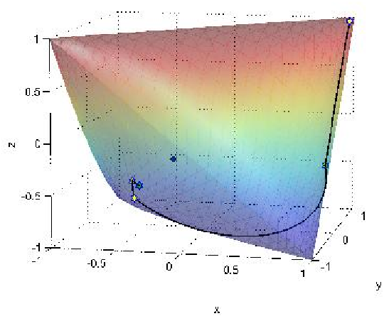
1. The details of this representation are given in Section 6.2. The blue point in the center and the green point represent, respectively, the target matrix and the solution point . As the figure suggests, the algorithm has fast convergence and the constraint set is a curved space.
This novel technique we propose, is based on geometric optimisation that can locally minimize the objective function in (1) and which incorporates the Hadamard semi-norm. In fact, our method can be applied to any sufficiently smooth objective function. Not all other methods available in the literature that aim to solve (1) can handle an arbitrary objective function, see the literature review in Section 2. We formulate the problem in terms of Riemannian geometry. This approach allows us to use numerical methods on manifolds that are numerically stable and efficient, in particular the Riemannian-Newton method is applied. We show, for the numerical tests we performed, that the numerical efficiency of geometric optimisation compares favourably to the other algorithms available in the literature. The only drawback of the practical use of geometric optimisation is that the implementation is rather involved. To overcome this drawback, we have made available a MATLAB implementation ‘LRCM min’ (low-rank correlation matrices minimization) at www.few.eur.nl/few/people/pietersz.
We develop a technique to instantly check whether an obtained local minimum is a global minimum, by adaptation of Lagrange multiplier results of ?. The novelty consists of an expression for the Lagrange multipliers given the matrix , whereas until now only the reverse direction (an expression for the matrix given the Lagrange multipliers) was known. The fact that one may instantly identify whether a local minimum is a global minimum is very rare for non-convex optimisation problems, and that makes Problem (1), which is non-convex for , all the more interesting.
Problem (1) is important in finance, as it occurs as part of the calibration of the multi-factor LIBOR11 1 London inter-bank offer rate. market model of ?, ?, ? and ?. This model is an interest rate derivatives pricing model and it is used in some financial institutions for valuation and risk management of their interest rate derivatives portfolio. The number of stochastic factors needed for the model to fit to the given correlation matrix is equal to the rank of the correlation matrix. This rank can be as high as the number of forward LIBORs in the model, i.e., as high as the dimension of the matrix. The number of LIBORs in the model can grow large in practical applications, for example, a model with over 80 LIBORs is not uncommon. This implies that the number of factors needed to fit the model to the given correlation matrix can be high, too. There is much empirical evidence that the term structure of interest rates is driven by multiple factors (three, four, or even more), see the review article of ?. Though the number of factors driving the term structure may be four or more, the empirical work shows that it is certainly not as high as, say, 80. This is one reason for using a model with a low number of factors. Another reason is the enhanced efficiency when estimating the model-price of an interest rate derivative through Monte Carlo simulation. First, a lower factor model simply requires drawing less random numbers than a higher factor model. Second, the complexity of calculating LIBOR rates over a single time step in a simulation implementation is of order , with the number of LIBORs and the number of factors, see ?.
The importance of Problem (1) in finance has been recognized by many researchers. In fact, the literature review of Section 2 refers to seventeen articles or books addressing the problem.
Due to its generality our method finds locally optimal points for a variety of other objective functions subject to the same constraints. One of the most famous problems comes from physics and is called Thomson’s problem. The Thomson problem is concerned with minimizing the potential energy of charged particles on the sphere in (). Geometric optimisation techniques have previously been applied to the Thomson problem by ?, but these authors have only considered conjugate gradient techniques on a ‘bigger’ manifold, in which the freedom of rotation has not been factored out. In comparison, we stress here that our approach considers a lower dimensional manifold, which allows for Newton’s algorithm (the latter not developed in ?). An implementation of geometric optimisation applied to the Thomson problem has also been included in the ‘LRCM min’ package.
Finally, for a literature review of interest rate models, the reader is referred to ?.
The paper is organized as follows. In Section 2, the literature is reviewed. In Section 3, the constraints of the problem are formulated in terms of differential geometry. We parameterize the set of correlation matrices of rank at most with a manifold named the Cholesky manifold. This is a canonical space for the optimisation of the arbitrary smooth function subject to the same constraints. In Section 4, the Riemannian structure of the Cholesky manifold is introduced. Formulas are given for parallel transport, geodesics, gradient and Hessian. These are needed for the minimization algorithms, which are made explicit. In Section 5, we discuss the convergence of the algorithms. In Section 6, the application of the algorithms to the problem of finding the nearest low-rank correlation matrix is worked out in detail. In Section 7, we numerically investigate the algorithms in terms of efficiency. Finally, in Section 8, we conclude the paper.
2 Literature review
We mention five algorithms available in the literature for rank reduction of correlation matrices, in reverse chronological order.
First, we mention the majorization approach of ?. This reference also contains a literature review covering all algorithms except for the alternating projections algorithm (discussed below). Majorization can handle an entry-weighted objective function and is guaranteed to converge to a stationary point. The rate of convergence is sub-linear.
Second, we point out the Lagrange multiplier algorithm of ? and ?. The correlation matrices produced by this algorithm are not guaranteed to converge to a stationary point of objective function in (1). This lack of convergence has been pointed out in ? and therefore it is not necessary to repeat the reasons here.
Third, we consider the alternating projections algorithm of ? and ?. The discussion below of alternating projections applies only to the problem of rank reduction of correlation matrices. The method is based on alternating projections onto the set of matrices with unit diagonal and onto the set of matrices of rank or less. Both these projections can be efficiently calculated. For projection onto the intersection of two convex sets, ? and ? have shown that convergence to a minimum can be obtained with alternating projections onto the individual convex sets if a normal vector correction is applied. Their results do not automatically hold for an alternating projections algorithm with normal correction for Problem (1)22 2 The algorithm with normal correction for rank reduction has also been studied in ?., since for the set of matrices of rank or less is non-convex. Indeed, ? and ? report that alternating projections with normal correction may fail in solving Problem (1). The alternating projections algorithm without normal correction stated in ? and ? however always converges to a feasible point, but not necessarily to a stationary point. In fact, in general, the alternating projections method without normal correction does not converge to a stationary point. The algorithm thus does not minimize the objective function in (1), it only selects a feasible point satisfying the constraints of (1).
The fourth important contribution is due to ?. The algorithm of ? is the alternating projection algorithm with normal correction applied to the case , i.e., to the problem of finding the nearest (possibly full-rank) correlation matrix. Note that the space of positive semidefinite matrices of rank is indeed convex, therefore the alternating projections with normal correction method is guaranteed to converge to the global minimum. Since the case is of primary interest in this paper, the alternating projections method with normal correction will not be considered in the remainder.
Fifth, we mention the parametrization method of ?, ?, ? and ?. The set of correlation matrices of rank or less is parameterized by trigonometric functions through spherical coordinates with . As a result, the objective value becomes a function of the angle parameters that live in . Subsequently, ordinary non-linear optimisation algorithms may be applied to minimize the objective value over the angle parameters . In essence, this approach is the same as geometric optimisation, except for the key difference of optimising over versus over . The major benefit of geometric optimisation over the parametrization method is as follows. Consider, for ease of exposition, the case of equal weights. The differential , in terms of , is given simply as , with , see (25) below. Note that can thus be efficiently calculated. The differential , in terms of however, is multiplied by the differential of with respect to , by the chain rule of differentiation. The latter differential is less efficient to calculate since it involves numerous sums of trigonometric functions.
An initial feasible point can be found by a principal component analysis and a suitable re-scaling. This method is explained in Section 6.5 below, and is due to ?. It first appeared in a finance setting in ? and ?. The starting point for the five above mentioned algorithms is the re-scaled PCA initial feasible point.
2.1 Weighted norms
We mention two reasons for assigning non-constant or non-homogeneous weights in the objective function of (2). First, in our setting has the interpretation of measured correlation. It can thus be the case that we are more confident of specific entries of the matrix . Second, the weighted norm of (2) has important applications in finance, see, for example, ?, ? and ?.
The semi-norm in the objective function can be (i) a Hadamard semi-norm with arbitrary weights per element of the matrix, as defined in (2), or (ii) a weighted Frobenius norm with a positive definite matrix. Here . The weighted Frobenius norm is, from a practical point of view, by far less transparent than the Hadamard or weights-per-entry semi-norm (2). The geometric optimisation theory developed in this paper, and most of the algorithms mentioned in Section 2, can be efficiently applied to both cases. The Lagrange multipliers and alternating projections methods however can only be efficiently extended to the case of the weighted Frobenius norm. The reason is that both these methods need to calculate a projection onto the space of matrices of rank or less. Such a projection, for the weighted Frobenius norm, can be efficiently found by an eigenvalue decomposition. For the Hadamard semi-norm, such an efficient solution is not available, to our knowledge, and as also mentioned in ?.
3 Solution methodology with geometric optimisation
Note that Problem (1) is a special case of the following more general problem:
|
(3) |
In this paper methods will be developed to solve Problem (3) for the case when is twice continuously differentiable. In the remainder of the paper, we assume , since for the constraint set consists of a finite number ( of points.
3.1 Basic idea
The idea for solving Problem (3) is to parameterize the constraint set by a manifold, and subsequently utilize the recently developed algorithms for optimisation over manifolds, such as Newton’s algorithm and conjugate gradient algorithms. Such geometric optimisation has been developed by ?.
In Section 3.2, the constraint set is equipped with a topology, and we make an identification with a certain quotient space. In Section 3.3, it will be shown that the constraint set as such is not a manifold; however a dense subset is shown to be a manifold, namely the set of matrices of rank exactly . Subsequently, in Section 3.4, we will define a larger manifold (named Cholesky manifold), of the same dimension as the rank- manifold, that maps surjectively to the constraint set. We may apply geometric optimisation on the Cholesky manifold. The connection between minima on the Cholesky manifold and on the constraint set will be established.
3.2 Topological Structure
In this section, the set of correlation matrices of rank or less is equipped with the subspace topology from . We subsequently establish a homeomorphism (i.e., a topological isomorphism) between the latter topological space and the quotient space of products of the sphere over the group of orthogonal transformations of . Intuitively the correspondence is as follows: We can associate with an correlation matrix of rank a configuration of points of unit length in such that the inner product of points and is entry of the correlation matrix. Any orthogonal rotation of the configuration does not alter the associated correlation matrix. This idea is developed more rigorously below.
Definition 1.
The set of symmetric correlation matrices of rank at most is defined by
Here denotes the identity matrix and denotes the map , , where denotes the Kronecker delta.
The set is a subset of . The latter space is equipped with the Frobenius norm , which in turn defines a topology. We equip with the subspace topology.
In the following, the product of unit spheres is denoted by . Elements of are denoted as a matrix , with each row vector of unit length. Denote by the group of orthogonal transformations of -space. Elements of are denoted by a orthogonal matrix .
Definition 2.
We define the following right -action33 3 It is trivially verified that the map thus defined is indeed an smooth action: and . Standard matrix multiplication is smooth. on :
| (4) |
An equivalence class associated with is denoted by and it is called the orbit of . The quotient space is denoted by . The canonical projection is denoted by . Define the map44 4 Although rather obvious, it will be shown in Theorem 3 that this map is well defined. as
Consider a map in the inverse direction of ,
defined as follows: For take such that . Such can always be found as will be shown in Theorem 3 below. Then set . It will be shown in Theorem 3 that this map is well defined. Finally, define the map , .
The following theorem relates the spaces and ; the proof has been deferred to Appendix A.
3.3 A dense part of equipped with a differentiable structure
For an exposition on differentiable manifolds, the reader is referred to ?. It turns out that is not a manifold, but a so-called stratified space, see, e.g., ?. However there is a subspace of that is a manifold, which is the manifold of equivalence classes of matrices of exactly rank . The proof of the following proposition has been deferred to Appendix B.
Proposition 4.
Let be the subspace defined by
Then we have the following:
- 1.
is a sub-manifold of .
- 2.
Denote by the quotient space . Then is a manifold of dimension .
As shown in Proposition 4, a subset of is a manifold. In the following, we will study charts given by sections of the manifold that will ultimately lead to the final manifold over which will be optimized.
A section on is a map , with open in , such that . Such a map singles out a unique matrix in each equivalence class. In our case we can explicitly give such a map . Let in , and let denote a subset of with exactly elements, such that , for . Note that is well defined since any two are coupled by an orthogonal transformation, see the proof of Theorem 3, and orthogonal transformations preserve independence. The collection of all such is denoted by . It is readily verified that is not empty. Let denote the lexicographical ordering, then is a well-ordered set. Thus we can choose the smallest element, denoted by . Define by taking the rows of from , thus . Define . Since is positive definite, Cholesky decomposition can be applied to , see for example ?, to obtain a unique lower-triangular matrix such that and . By Theorem 3, there exists a unique orthogonal matrix such that . Define . Note that is lower-triangular, since for , let be the largest integer such that , then is dependent on , as is the smallest element from , which implies a lower-triangular form for . Then define . It is obvious that and are open in the corresponding topologies. Then
| (6) |
is a section of at . The following proposition shows that the sections are the charts of the manifold . The proof has been deferred to Appendix C.
Proposition 5.
The differentiable structure on is the one which makes into a diffeomorphism.
3.4 The Cholesky manifold
In this section, we will show that, for the purpose of optimisation, it is sufficient to perform the optimisation on a compact manifold that contains one of the sections. For simplicity we choose the section where . The image is a smooth sub-manifold of with the following representation in
with embedded in by the first coordinates such that coordinate is bigger than and with the remaining coordinates set to zero. Also, is similarly embedded in . We can consider the map restricted to , which is differentiable since is a sub-manifold of . The map is a homeomorphism, in virtue of Theorem 3.
For the purpose of optimisation, we need a compact manifold which is surjective with . Define the following sub-manifold of of dimension ,
which we call the Cholesky manifold. The Cholesky parametrization has been considered before by ?, but these authors do not consider non-Euclidean geometric optimisation. The map is surjective, in virtue of the following theorem, the proof of which has been relegated to Appendix D.
Theorem 6.
If , then there exists a such that .
A function on can be considered on , too, via the composition
From here on, we will write viewed as a function on .
For a global minimum on , we have that attains a global minimum of on , since the map is surjective. For a local minimum, we have the following theorem. The proof has been deferred to Appendix E.
Theorem 7.
The point attains a local minimum of on if and only if attains a local minimum of on .
These considerations on global and local minima on show that, to optimize over , we might as well optimize over the manifold . For the optimisation of over , there is no straightforward way to use numerical methods such as Newton and conjugate gradient, since they require a notion of differentiability, but for optimisation of on , we can use such numerical methods.
3.5 Choice of representation
In principle, we could elect another manifold and a surjective open map . We insist however on explicit knowledge of the geodesics and parallel transport, for this is essential to obtaining an efficient algorithm. We found that if we choose the Cholesky manifold then convenient expressions for geodesics, etc., are obtained. Moreover, the Cholesky manifold has the minimal dimension, i.e., .
In the next section, the geometric optimisation tools are developed for the Cholesky manifold.
4 Optimisation over the Cholesky manifold
For the development of minimization algorithms on a manifold, certain objects of the manifold need to calculated explicitly, such as geodesics, parallel transport, etc. In this section, these objects are introduced and made explicit for .
From a theoretical point of view, it does not matter which coordinates we choose to derive the geometrical properties of a manifold. For the numerical computations however this choice is essential because the simplicity of formulas for the geodesics and parallel transport depends on the chosen coordinates. We found that simple expressions are obtained when is viewed as a sub-manifold of , which, in turn, is viewed as a subset of the ambient space . This representation reveals that, to calculate geodesics and parallel transport on , it is sufficient to calculate these on a single sphere.
The tangent space of the manifold at a point is denoted by . A tangent vector at a point is an element of and is denoted by .
4.1 Riemannian structure
We start with a review of basic concepts of Riemannian geometry. Our exposition follows ?. Let be an -dimensional differentiable manifold. A Riemannian structure on is a smooth map , which for every assigns an inner product on , the tangent space at point . A Riemannian manifold is a differentiable manifold with a Riemannian structure.
Let be a smooth function on a Riemannian manifold . Denote the differential of at a point by . Then is a linear functional on . In particular, let , , be a smooth curve on such that and expressed in a coordinate chart is equal to , then can be expressed in this coordinate chart by
| (7) |
The linear space of linear functionals on (the dual space) is denoted by . A vector field is a map on that selects a tangent at each point . The Riemannian structure induces an isomorphism between and , which guarantees the existence of a unique vector field on , denoted by , such that
| (8) |
This vector field is called the gradient of . Also, for Newton and conjugate gradient methods, we have to use second order derivatives. In particular, we need to be able to differentiate vector fields. To do this on a general manifold, we need to equip the manifold with additional structure, namely the connection. A connection on a manifold is a rule which assigns to each two vector fields on a vector field on , satisfying the following two conditions:
| (9) |
for smooth functions on and vector fields on .
Let be a smooth curve on with tangent vector . A given family of tangent vectors at the points is said to be parallel transported along if
| (10) |
where are vector fields that coincide with and , respectively, on . If the tangent vector itself is parallel transported along then the curve is called a geodesic. In particular, if is a coordinate chart on and the corresponding vector fields then the affine connection on can be expressed by
| (11) |
The functions are smooth functions, called the Christoffel symbols for the connection. In components, the geodesic equation becomes
| (12) |
where are the coordinates of . On a Riemannian manifold there is a unique torsion free connection compatible with the metric, called the Levi-Civita connection. This means that Christoffel symbols can be expressed as functions of a metric on . Note also that (12) implies that, once we have determined the equation for the geodesic we can simply read off Christoffel symbols. With respect to an induced metric the geodesic is the curve of shortest length between two points on a manifold. For a manifold embedded in Euclidean space an equivalent characterization of a geodesic is that the acceleration vector at each point along a geodesic is normal to the manifold so long as the curve is traced with uniform speed.
We start by defining Riemannian structures for and for the Cholesky manifold . We use the Levi-Civita connection, associated to the metric defined as follows on the tangent spaces. Both tangent spaces are identified with suitable subspaces of the ambient space , and subsequently the inner product for two tangents , is defined as
| (13) |
which is the Frobenius inner product for matrices. Note that, in our special case, the inner product is independent of the point ; therefore we suppress the dependency on .
4.2 Normal and tangent spaces
An equation determining tangents to at a point can be obtained by differentiating yielding , i.e., . The dimension of the tangent space is . The normal space at the point is defined to be the orthogonal complement of the tangent space at the point , i.e., it consists of the matrices , for which for all in the tangent space. It follows that the normal space is dimensional. It is straightforward to verify that if , where is diagonal, then is in the normal space. Since the dimension of the space of such matrices is , we see that the normal space at is given by
The projections and onto the normal and tangent spaces of are given by
respectively. The projection onto the tangent space of is given by
| (14) |
4.3 Geodesics
It is convenient to work with the coordinates of the ambient space . In this coordinate system, geodesics on with respect to the Levi-Civita connection obey the second order differential equation
| (15) |
To see this, we begin with the condition that remains on ,
| (16) |
Differentiating this equation twice, we obtain,
| (17) |
In order for to be a geodesic, must be in the normal space at , i.e.,
| (18) |
for some diagonal matrix . To obtain an expression for , substitute (18) into (17), which yields (15).
The function is the matrix notation of the Christoffel symbols, , with respect to , the standard basis vectors of . More precisely, with defined by .
The geodesic at in the direction is given by,
| (19) |
for , per component on the sphere. By differentiating, we obtain an expression for the evolution of the tangent along the geodesic:
| (20) |
Since is a Riemannian sub-manifold of it has the same geodesics.
4.4 Parallel transport along a geodesic
We consider this problem per component on the sphere. If is parallel transported along a geodesic starting from in the direction of , then decompose in terms of ,
Then changes according to (20) and remains unchanged. Parallel transport from to defines an isometry . When it is clear in between which two points is transported, then parallel transport is denoted simply by . Since is a Riemannian sub-manifold of it has the same equations for parallel transport.
4.5 The gradient
Since is a sub-manifold of we can use coordinates of to express the differential of at the point , namely . The gradient of a function on can be determined by (8). It follows that,
| (21) |
4.6 Hessian
The Hessian of a function is a second covariant derivative of . More precisely, let be two vector fields, then
In local coordinates of
| (22) |
where
Newton’s method requires inverting the Hessian at minus the gradient, therefore we need to find the tangent to such that
| (23) |
To solve (23), it is convenient to calculate the unique tangent vector satisfying
since then the Newton Equation (23) becomes . From (15) and (22), we obtain
| (24) |
where the notation means the tangent vector satisfying
4.7 Algorithms
We are now in a position to state the conjugate gradient algorithm, given as Algorithm 1, and the Newton algorithm, given as Algorithm 2, for optimisation over the Cholesky manifold. These algorithms are instances of the geometric programs presented in ?, for the particular case of the Cholesky manifold.
5 Discussion of convergence properties
In this section, we discuss convergence properties of the geometric programs: global convergence and the local rate of convergence.
5.1 Global convergence
First, we discuss global convergence for the Riemannian-Newton algorithm. It is well known that the Newton algorithm, as displayed in Algorithm 2, is not globally convergent to a local minimum. Moreover, the steps in Algorithm 2 may even not be well defined, because the Hessian mapping could be singular. The standard way to resolve these issues, is to introduce jointly a steepest descent algorithm. So Algorithm 2 is adjusted in the following way. When the new search direction has been calculated, then we also consider the steepest descent search direction . Subsequently, a line minimization of the objective value is performed in both directions, and . We then take as the next point of the algorithm whichever search direction finds the point with lowest objective value. Such a steepest descent method with line minimization is well known to have guaranteed convergence to a local minimum.
Second, we discuss global convergence for conjugate gradient algorithms. For the Riemannian case, we have not seen any global convergence results for conjugate gradient algorithms in the literature. Therefore we focus on the results obtained for the flat-Euclidean case. ? and ? establish global convergence of the ? conjugate gradient method with line minimization. ? establish alternative line search minimizations that guarantee global convergence of the ? conjugate gradient method.
Input: .
Input: .
5.2 Local rate of convergence
Local rates of convergence for geometric optimisation algorithms are established in ?, ? and ?.
In Theorem 3.3 of ?, the following result is established for the Riemannian-Newton method. If is a non-degenerate stationary point, then there exists an open set containing , such that starting from any in , the sequence of points produced by Algorithm 2 converges quadratically to .
In Theorem 4.3 of ?, the following result is stated for the Riemannian ? and ? conjugate gradient methods. Suppose is a non-degenerate stationary point such that the Hessian at is positive definite. Suppose is a sequence of points, generated by Algorithm 1, converging to . Then, for sufficiently large , the sequence has -steps quadratic convergence to .
As a numerical illustration, convergence runs have been displayed in Figure

2, for reducing a correlation matrix to rank 3. The following algorithms are compared:
- 1.
Steepest descent, for which the search direction in Algorithm 1 is equal to , i.e., to minus the gradient. The steepest descent method has a linear local rate of convergence, see ?.
- 2.
PRCG, Polak-Ribière conjugate gradient.
- 3.
FRCG, Fletcher-Reeves conjugate gradient.
- 4.
Newton.
- 5.
Lev.-Mar., the ? & ? method, which is a Newton-type method.
The code that is used for this test is the package ‘LRCM min’, to be discussed in Section 7. This package also contains the correlation matrix used for the convergence run test. Figure 2 clearly illustrates the convergence properties of the various geometric programs. The efficiency of the algorithms is studied in Section 7 below.
6 A special case: Distance minimization
In this section, the primary concern of this paper to minimize the objective function of (2) is studied. The outline of this section is as follows. First, some particular choices for and are examined. Second, the differential and Hessian of are calculated. Third, the connection with Lagrange multipliers is stated; in particular, this will lead to an identification method of whether a local minimum is a global minimum. Fourth, we discuss the PCA with re-scaling method for obtaining an initial feasible point.
6.1 The case of
The case that is a symmetric matrix and the closest positive semidefinite matrix is to be found allows a successive projection solution, which was shown by ?.
6.2 The case of ,
A symmetric matrix with ones on the diagonals is denoted by
Its determinant is given by
By straightforward calculations it can be shown that implies that all eigenvalues are nonnegative. The set of 3 by 3 correlation matrices of rank 2 may thus be represented by the set . To get an intuitive understanding of the complexity of the problem, the feasible region has been displayed in Figure 1.
6.3 Formula for the differential of
Consider the specific case of the weighted Hadamard semi-norm of (2). This semi-norm can be represented by a Frobenius norm by introducing the Hadamard product . The Hadamard product denotes entry-by-entry multiplication. Formally, for two matrices and of equal dimensions, the Hadamard product is defined by . The objective function (2) can then be written as
with and with . Then
Thus from (7) we have
| (25) |
Similarly, we may compute the second derivative
with any curve starting from in the direction of .
6.4 Connection normal with Lagrange multipliers
The following lemma provides the basis for the connection of the normal vector at versus the Lagrange multipliers of the algorithm of ? and ?. The result is novel since previously only an expression was known for the matrix given the Lagrange multipliers. The result below establishes the reverse direction. This Lagrange result will allow us to identify whether a local minimum is also a global minimum. That we are able to efficiently determine whether a local minimum is a global minimum, is a very rare phenomenon in non-convex optimisation, and makes the rank reduction problem (non-convex for ) all the more interesting.
Note that the Lagrange theory is based on an efficient expression of the low-rank projection by an eigenvalue decomposition. Therefore the theory below can be extended efficiently only for the Hadamard norm with equal weights and for the weighted Frobenius norm, see also the discussion in Section 2.1. The proof of the following lemma has been deferred to Appendix F.
Lemma 8.
Let be such that . Here, is the gradient of on , , with in (25). Define
and define . Then there exist a joint eigenvalue decomposition
where can be obtained by selecting at most nonnegative entries from (here if an entry is selected it retains the corresponding position in the matrix).
The characterization of the global minimum for Problem (1) was first achieved in ? and ?, which we repeat here: Denote by a matrix obtained by eigenvalue decomposition of together with leaving in only the largest eigenvalues (in absolute value). Denote for : . The proof of the following theorem has been repeated for clarity in Appendix G.
Theorem 9.
This brings us in a position to identify whether a local minimum is a global minimum:
Theorem 10.
6.5 Initial feasible point
To obtain an initial feasible point we use a method of ?. We first perform an eigenvalue decomposition
| (27) |
Then we define by assigning to each row
where consists of the first columns of and where is the principal sub-matrix of of degree , filled only with the non-negative elements from . The scaling is to ensure that each row of is of unit length. If row is a priori of zero length, then we choose to be an arbitrary vector in of unit length. Finally, to obtain an initial feasible point in , we perform a Cholesky decomposition as in the proof of Theorem 6.
7 Numerical results
There are many different algorithms available in the literature, as detailed in Section 2. Some of these have an efficient implementation, i.e., the cost of a single iteration is low. Some algorithms have fast convergence, for example, the Newton method has quadratic convergence. Algorithms with fast convergence usually require less iterations to attain a predefined convergence criterion. Thus, the real-world performance of an algorithm is a trade-off between cost-per-iterate and number of iterations required. A priori, it is not clear which algorithm will perform best. Therefore, in this section, the numerical performance of geometric optimisation is compared to other methods available in the literature.
7.1 Acknowledgement
Our implementation of geometric optimisation over low-rank correlation matrices ‘LRCM min’55 5 LRCM min can be downloaded from www.few.eur.nl/few/people/pietersz. is an adoption of the ‘SG min’ template of ? (written in MATLAB) for optimisation over the Stiefel and Grassmann manifolds. This template contains four distinct well-known non-linear optimisation algorithms adapted for geometric optimisation over Riemannian manifolds: Newton algorithm; dogleg step or ? and ? algorithm; ? conjugate gradient; and ? conjugate gradient.
7.2 Numerical comparison
The performances of the following seven algorithms, all of these described in Sections 4 and 2, except for item 7 (fmincon), are compared:
- 1.
Geometric optimisation, Newton (Newton).
- 2.
Geometric optimisation, Fletcher-Reeves conjugate gradient (FRCG).
- 3.
Majorization, e.g., ? (Major.).
- 4.
Parametrization, e.g., ? (Param.).
- 5.
Alternating projections without normal vector correction, e.g., ? (Alt. Proj.).
- 6.
Lagrange multipliers, e.g., ? (Lagrange).
- 7.
fmincon, a MATLAB built-in medium-scale constrained nonlinear program (fmincon).
Note that the first two algorithms in this list have been developed in this paper. The algorithms are tested on a large number of randomly generated correlation matrices. The benefit of testing on many correlation matrices is, that the overall and generic performance of the algorithms may be assessed. The correlation matrices are randomly generated as follows. A parametric form for (primarily interest rate) correlation matrices is posed in ?. We repeat the parametric form here for completeness.
with and with denoting the expiry time of rate . (Our particular choice is , ) This model was then subsequently estimated with USD historical interest rate data. In Table 3 of ? the estimated -parameters are listed, along with their standard error. An excerpt of this table has been displayed in Table 1.
| estimate | 0.000 | 0.480 | 1.511 | 0.186 |
| standard error | - | 0.099 | 0.289 | 0.127 |
The random correlation matrix that we use is obtained by randomizing the -parameters. We assume the -parameters distributed normally with mean and standard errors given by Table 1, with capped at zero.
As the benchmark criterion for the performance of an algorithm, we take its obtained accuracy of fit given a fixed amount of computational time. Such a criterion corresponds to financial practice, since decisions based on derivative valuation calculations often need to be made within seconds. To display the comparison results, we use the state-of-the-art and convenient performance profiles; see ?. The reader is referred there for details, but the idea is briefly described here. There are 100 test correlation matrices and seven algorithms . As performance measure we take the obtained function value of algorithm on problem given the limited computational time. The performance ratio is defined to be the ratio of the performance measure of the algorithm over the best obtained performance measure for all seven algorithms,
The cumulative distribution function of the performance ratio for algorithm , viewed as a random variable , is then the performance profile of algorithm ,
A rule of thumb is, that the higher the profile of an algorithm, the better its performance. The performance profiles have been displayed in Figures


3–6, for various choices of , , and computational times. Each performance profile represents a benchmark on 100 different test interest rate correlation matrices. For Figures 3–5, an objective function with equal weights is used. For Figure 6, we use a Hadamard semi-norm with non-constant weights. These weights are chosen so as to reflect the importance of the correlation entries for a specific trigger swap, as outlined in, e.g., ?. For this specific trigger swap, the first three rows and columns are important. Therefore the weights matrix takes the form
8 Conclusions
We applied geometric optimisation tools for finding the nearest low-rank correlation matrix. The differential geometric machinery provided us with an algorithm more efficient than any existing algorithm in the literature, at least for the numerical cases considered. The geometric approach also allows for insight and more intuition into the problem. We established a technique that allows one to straightforwardly identify whether a local minimum is a global minimum.
References
- [2] [] Abraham, R., Marsden, J. E. & Ratiu, T. (1988), Manifolds, Tensor Analysis, and Applications, Springer-Verlag, Berlin.
- [4] [] Al-Baali, M. (1985), ‘Descent property and global convergence of the Fletcher-Reeves method with inexact line search’, IMA Journal of Numerical Analysis 5, 121–124.
- [6] [] Brace, A., Ga̧tarek, D. & Musiela, M. (1997), ‘The market model of interest rate dynamics’, Mathematical Finance 7(2), 127–155.
- [8] [] Brigo, D. (2002), A note on correlation and rank reduction, www.damianobrigo.it.
- [10] [] Brigo, D. & Mercurio, F. (2001), Interest Rate Models: Theory and Practice, Springer-Verlag, Berlin.
- [12] [] do Carmo, M. P. (1992), Riemannian Geometry., 12 edn, Birkhäuser, Boston, MA.
- [14] [] Dai, Q. & Singleton, K. (2003), ‘Term structure dynamics in theory and reality’, Review of Financial Studies 16(3), 631–678.
- [16] [] De Jong, F., Driessen, J. & Pelsser, A. A. J. (2004), ‘On the information in the interest rate term structure and option prices’, Review of Derivatives Research 7(2), 99–127.
- [18] [] Dedieu, J.-P., Priouret, P. & Malajovich, G. (2003), ‘Newton’s method on Riemannian manifolds: Covariant alpha-theory’, IMA Journal of Numerical Analysis 23(3), 395–419.
- [20] [] Depczynski, U. & Stöckler, J. (1998), A differential geometric approach to equidistributed knots on Riemannian manifolds, in C. K. Chui & L. L. Schumaker, eds, ‘Approximation Theory IX, Theoretical Aspects’, Vol. 1, Vanderbilt University Press, Nashville, TN, pp. 99–106.
- [22] [] Dolan, E. D. & Moré, J. J. (2002), ‘Benchmarking optimization software with performance profiles’, Mathematical Programming, Series A 91(2), 201–213.
- [24] [] Duistermaat, J. J. & Kolk, J. A. C. (2000), Lie Groups, Springer-Verlag, Berlin.
- [26] [] Dykstra, R. L. (1983), ‘An algorithm for restricted least squares regression’, Journal of the American Statistical Association 87(384), 837–842.
- [28] [] Edelman, A. & Lippert, R. (2000), Nonlinear eigenvalue problems with orthogonality constraints (section 8.3), in Z. Bai, J. Demmel, J. Dongarra, A. Ruhe & H. van der Vorst, eds, ‘Templates for the Solution of Algebraic Eigenvalue Problems: A Practical Guide’, SIAM, Philidelphia, NJ.
- [30] [] Edelman, A., Arias, T. A. & Smith, S. T. (1998), ‘The geometry of algorithms with orthogonality constraints’, SIAM Journal of Matrix Analysis and its Applications 20(2), 303–353.
- [32] [] Fletcher, R. & Reeves, C. M. (1964), ‘Function minimization by conjugate gradients’, Computer Journal 7(2), 149–154.
- [34] [] Flury, B. (1988), Common Principal Components and Related Multivariate Models, J. Wiley & Sons, New York.
- [36] [] Gilbert, J.-C. & Nocedal, J. (1992), ‘Global convergence properties of conjugate gradient methods for optimization’, SIAM Journal on Optimization 2(1), 21–42.
- [38] [] Golub, G. H. & van Loan, C. F. (1996), Matrix Computations, 3 edn, John Hopkins University Press, Baltimore, MD.
- [40] [] Grubišić, I. (2002), Interest rate theory: BGM model, Master’s thesis, Leiden University. www.math.uu.nl/people/grubisic.
- [42] [] Han, S.-P. (1988), ‘A successive projection method’, Mathematical Programming 40, 1–14.
- [44] [] Higham, N. J. (2002), ‘Computing the nearest correlation matrix–a problem from finance’, IMA Journal of Numerical Analysis 22(3), 329–343.
- [46] [] Horn, R. A. & Johnson, C. R. (1990), Matrix Analysis, Cambridge University Press, Cambridge.
- [48] [] Hull, J. C. & White, A. (2000), ‘Forward rate volatilities, swap rate volatilities, and implementation of the LIBOR market model’, Journal of Fixed Income 10(2), 46–62.
- [50] [] Jamshidian, F. (1997), ‘LIBOR and swap market models and measures’, Finance and Stochastics 1(4), 293–330.
- [52] [] Joshi, M. S. (2003), ‘Rapid computation of drifts in a reduced factor LIBOR market model’, Wilmott Magazine 5, 84–85.
- [54] [] Levenberg, K. (1944), ‘A method for the solution of certain non-linear problems in least squares’, Quarterly of Applied Mathematics 2, 164–168.
- [56] [] Marquardt, D. W. (1963), ‘An algorithm for least-squares estimation of nonlinear parameters’, Journal of the Society for Industrial and Applied Mathematics 11(2), 431–441.
- [58] [] Miltersen, K. R., Sandmann, K. & Sondermann, D. (1997), ‘Closed form solutions for term structure derivatives with log-normal interest rates’, Journal of Finance 52(1), 409–430.
- [60] [] Morini, M. & Webber, N. (2004), An EZI method to reduce the rank of a correlation matrix, www.cass.city.ac. uk/facfin/facultypages/nwebber/.
- [62] [] Munkres, J. R. (1975), Topology, Prentice-Hall, London.
- [64] [] Musiela, M. & Rutkowski, M. (1997), ‘Continuous-time term structure models: Forward measure approach’, Finance and Stochastics 1(4), 261–291.
- [66] [] Pietersz, R. & Groenen, P. J. F. (2004a), ‘A major LIBOR fit’, Risk Magazine. December issue.
- [68] [] Pietersz, R. & Groenen, P. J. F. (2004b), ‘Rank reduction of correlation matrices by majorization’, Quantitative Finance. Forthcoming.
- [70] [] Polak, E. & Ribière, G. (1969), ‘Note sur la convergence de méthodes de directions conjuguées’, Revue Française d’Informatique et de Recherche Opérationnelle 16, 35–43.
- [72] [] Rapisarda, F., Brigo, D. & Mercurio, F. (2002), Parametrizing correlations: A geometric interpretation, Banca IMI Working Paper, www.fabiomercurio.it.
- [74] [] Rebonato, R. (1999a), ‘Calibrating the BGM model’, Risk Magazine, pp. 74–79. March.
- [76] [] Rebonato, R. (1999b), ‘On the simultaneous calibration of multifactor lognormal interest rate models to Black volatilities and to the correlation matrix’, Journal of Computational Finance 2(4), 5–27.
- [78] [] Rebonato, R. (1999c), Volatility and Correlation in the Pricing of Equity, FX and Interest-Rate Options, J. Wiley & Sons, Chichester.
- [80] [] Rebonato, R. (2002), Modern Pricing of Interest-Rate Derivatives, Princeton University Press, New Jersey.
- [82] [] Rebonato, R. (2004a), ‘Interest-rate term-structure pricing models: a review’, Proceedings of the Royal Society London 460, 667–728. Series A.
- [84] [] Rebonato, R. (2004b), Volatility and Correlation: The Perfect Hedger and the Fox, 2 edn, J. Wiley & Sons, Chichester, UK.
- [86] [] Sidenius, J. (2000), ‘LIBOR market models in practice’, Journal of Computational Finance 3(3), 5–26.
- [88] [] Smith, S. T. (1993), Geometric Optimization Methods for Adaptive Filtering, PhD thesis, Harvard University, Cambridge, MA.
- [90] [] Weigel, P. (2004), ‘Optimal calibration of LIBOR market models to correlations’, Journal of Derivatives (3).
- [92] [] Wu, L. (2003), ‘Fast at-the-money calibration of the LIBOR market model using Lagrange multipliers’, Journal of Computational Finance 6(2), 39–77.
- [94] [] Zhang, Z. & Wu, L. (2003), ‘Optimal low-rank approximation to a correlation matrix’, Linear Algebra and its Applications 364, 161–187.
- [96] [] Zoutendijk, G. (1970), Nonlinear programming, computational methods, in J. Abadie, ed., ‘Integer and nonlinear programming’, pp. 37–86.
- [97]
Appendix A The proof of Theorem 3
Proof of (i). The maps and are well defined: To show that is well defined, we need to show that if , then . From the assumption, we have that . If follows that
which was to be shown.
To show that is well defined, we need to show:
- (A)
If then there exists such that .
- (B)
If , with then there exists such that .
Ad (A): Let
be an eigenvalue decomposition with for . Note that such a decomposition of the specified form is possible because of the restriction . Then note that
Thus if we set then and , which was to be shown.
Ad (B): Let . Without loss of generality, we may assume that the first rows of and are independent. We extend the set of row vectors to a set of row vectors , such that the latter forms a basis of . Similarly, we obtain a basis of . It follows that there exists an orthogonal rotation , , such that , . Note that then also for , by linearity of and since the last row vectors are linearly dependent on the first row vectors by assumption. It follows that , which was to be shown.
Proof (ii). Diagram (5) is commutative: To show that : Let , then and and also . To show that : Let , then and and also .
Proof of (iii). The map is a homeomorphism with inverse : It is straightforward to verify that and are both the identity maps. The map is thus bijective with inverse . To show that is continuous, note that for quotient spaces we have: The map is continuous if and only if is continuous (see for example ?, Proposition 1.4.8). In our case, with is continuous. The proof now follows from a well-known lemma from topology: A continuous bijection from a compact space into a Hausdorff space is a homeomorphism (see for example ?, Theorem 5.6).
Appendix B Proof of Proposition 4
- 1.
It is sufficient to show that is open in , since is open in if and only if is open in . Since the rank of a symmetric matrix is a locally constant function, it follows that is an open subset of , with as in Definition 2.
- 2.
This part is a corollary of Theorem 1.11.4 of ?. This theorem essentially states that for a smooth action of a Lie group on a manifold the quotient is a manifold if the action is proper and free. First, we show that the action of on is proper66 6 For a definition, see ?.. Let
and a compact subset of . We have to show that is compact. By continuity of , is closed in . Because is bounded it follows that is compact.
Second, we show that the -action on is free. Let and such that . Since , it follows from the proof of Theorem 3 () that there exists precisely one such that . Thus, this must be the identity matrix.
The dimension of .
Appendix C Proof of Proposition 5
This part is a corollary of Theorem 1.11.4 of ?. This theorem states that there is only one differentiable structure on the orbit space which satisfies the following: Suppose that, for every , we have an open neighbourhood and a bijective map:
such that, for every , , . The differentiable structure on is the one which makes into a diffeomorphism. The topology of obtained in this manner is equal to the quotient topology.
Let and be a section over defined in (6). We define as follows. For , , there is a unique element such that . Then we define by . By definition, we have that . Since is a bijective map, we have that is bijective, too. It can be easily verified that satisfies the condition of Theorem 1.11.4 of ? stated above. It follows that is a diffeomorphism if and only if is a diffeomorphism. Thus, the differentiable structure on is the one which makes into a diffeomorphism.
Appendix D Proof of Theorem 6
Let and suppose that . Then there is a such that , by Theorem 3. Apply to the procedure77 7 The procedure in Section 3.3 is stated in terms of , but should be read there in this case. outlined in Section 3.3, to obtain a lower-triangular matrix , such that . A lower-triangular matrix that satisfies can now easily be obtained by setting
which was to be shown.
Appendix E Proof of Theorem 7
First, we prove the ‘only if’ part. Note that it is sufficient to show that the map is open. For then if attains a local minimum of on the open neighbourhood , then attains a local minimum of on the open neighbourhood of , since for any , .
To show that is open, note that it is sufficient to show that is open, since is a homeomorphism (see Proposition 4, item 3) and .
Suppose, then, that is open in . We have to show that is open in , by definition of the quotient topology of . We have
It is sufficient to show that the complement is closed. Let be a sequence in converging to , i.e. . We can write with and . Then,
| (28) |
Since is compact, there exists a convergent subsequence , with and , say. From (28) it follows that , which implies .
The reverse direction is obvious since the map is continuous.
Appendix F Proof of Lemma 8
It is recalled from matrix analysis that and admit a joint eigenvalue decomposition if and only if their Lie bracket equals zero. Define . Note that is the projection of onto the normal space at . Note also that
| (29) |
We calculate
| (30) |
The last equality follows from the assumption that , i.e. the differential is normal at . (Here, denotes the gradient on .) It follows from (30) and from the symmetry of that
- (i)
and also,
- (ii)
.
From (ii), and admit a joint eigenvalue decomposition, but then also jointly with because of (29). Suppose . From (i) we then have that and cannot both be non-zero. The result now follows since is positive semidefinite and has rank less than or equal to .
Appendix G Proof of Theorem 9
Define the Lagrangian
| (31) |
Note that the minimization problem in Equation (31) is attained by any (see e.g., Equation (30) of ?). For any ,
(This is the equation at the end of the proof of Theorem 4.4 of ?.) Here (in-)equality
- (a)
is obtained from the property that ,
- (b)
is by definition of , and
- (c)
is by assumption of (26).