Quantum first order phase transitions

Scaling theories are invaluable tools in the theory of quantum critical phenomena [1, 2]. They yield relations among the critical exponents governing the behavior of relevant thermodynamic quantities at very low temperatures. In the study of strongly correlated metals close to a quantum instability, they led to the discovery of a new characteristic temperature which marks the onset of Fermi liquid behavior [1]. Here we study the extension of scaling ideas to quantum first order phase transitions [3]. Although there is no diverging length in these transitions, this has proved to be very useful [4, 5, 6, 7] for temperature driven transitions and will turn out to be also the case for discontinuous quantum transitions.

Let us consider the scaling form of the $T=0$ free energy density close to the quantum phase transition,

$$f\propto|g|^{2-\alpha}$$

(1)

where $g$ measures the distance to the transition at $g=0$. The exponent $\alpha$ is related to the correlation exponent $\nu$ through the quantum hyperscaling relation $2-\alpha=\nu(d+z)$ [1] where $d$ is the dimension of the system and $z$ the dynamic critical exponent [3]. The total internal energy close to the transition can be written as,

$$U(g=0^{\pm})=U(g=0)\pm A_{\pm}|g|^{2-\alpha}$$

(2)

for $g\rightarrow 0^{\pm}$. Then the existence of a first order phase transition at $T=0$ with a discontinuity in $dU/dg$ and a latent heat implies the value $\alpha=1$ for this critical exponent. If quantum hyperscaling applies, this leads to a correlation length exponent $\nu=1/(d+z)$. This is the quantum equivalent of the classical result $\nu=1/d$ for temperature driven first order transitions [4, 5, 6, 7]. Associated with this value of the correlation length there is on the disordered side of the phase diagram a new energy scale, $T^{*}\propto|g|^{z/(d+z)}$.

The presence of a discontinuity in the order parameter and the assumption of no-decay of it’s correlation function imply $\beta=0$, as in the classical case [5] and $d+z-2+\eta=0$, respectively. As for classical transitions $\delta=\infty$ and for consistency with the scaling relations the order parameter susceptibility seems to diverge with an exponent $\gamma=1$ [5].

If the quantum transition is driven, for example, by pressure, $g\propto(P-P_{c})/P_{c}$ where $P_{c}$ is a critical pressure and a finite latent heat means in this case a finite amount of work, $W=A_{+}+A_{-}=P_{c}\Delta V$, to bring one phase into another. Such finite latent work is associated with a change in volume since the intensive variable, pressure in this case, remains constant at the transition. In the case of a density driven first order transition the chemical potential remains fixed while the number of particles changes.

In the next sections we study two problems which present first order quantum transitions and confirm the results obtained above on the basis of scaling arguments. These results are also important to clarify the meaning and the range of application of a scaling analysis in situations where criticality is in fact avoided.

An interesting case of a quantum first order transition occurs in a superconductor coupled to the electromagnetic field at $T=0$. The starting point to describe this transition is the Lagrangian density of charged particles minimally coupled to the electromagnetic field. The Lagrangian density of the model in given by,

	$\displaystyle L$	$\displaystyle=$	$\displaystyle-\frac{1}{4}(F_{\mu\nu})^{2}\!+\!\frac{1}{2}(\partial_{\mu}\varphi_{1}\!+\!qA_{\mu}\varphi_{2})^{2}+$		(3)
			$\displaystyle+\frac{1}{2}(\partial_{\mu}\varphi_{2}-qA_{\mu}\varphi_{1})^{2}+$
			$\displaystyle-\frac{1}{2}m^{2}(\varphi_{1}^{2}+\varphi_{2}^{2})-\frac{\lambda}{4!}(\varphi_{1}^{2}+\varphi_{2}^{2})^{2}$

where the first term is the Lagrangian of the electromagnetic field ($F_{\mu\nu}=\partial_{\mu}A_{\mu}-\partial_{\nu}A_{\nu}$) and the complex scalar field $\varphi$ associated with the superconducting state is given by, $\varphi=\frac{1}{\sqrt{2}}(\varphi_{1}+i\varphi_{2})$, with $\varphi_{1}$ and $\varphi_{2}$ real. At $T=0$ time enters as a new direction and the indices $\mu,\nu$ run from $0$ to $d=3$. The minimal coupling between these fields is through the electric charge $q$ and we are working in $\hbar=c=1$ units. This is essentially a quantum version of the Landau-Ginzburg free energy of a superconductor in a magnetic field [8]. As we are dealing with a Lorentz invariant case in which space and time enter on equal footing in the Lagrangian density, we can identify the dynamic critical exponent, $z=1$. For the chargeless problem ($q=0$) the Lagrangian above is associated with a quantum superfluid-insulator transition at $m^{2}=0$ as we discuss below. Furthermore, we are interested here in the case of spatial dimension $d=3$, such that, the effective dimension of the quantum problem is $d_{eff}=d+z=4$. The zero temperature effective potential associated with this Lagrangian density in the one-loop approximation is given by [3, 9],

$$V^{0}_{e\!f\!f}(\!\varphi_{c}\!)\!\!=\!\!\frac{m^{2}\varphi_{c}^{2}}{2}\!-\!\frac{m^{2}\varphi_{c}^{4}}{4\langle\varphi\rangle^{2}}\!+\!\frac{3q^{4}\varphi_{c}^{4}}{64\pi^{2}}[\ln(\frac{\varphi_{c}^{2}}{\langle\varphi\rangle^{2}})\!-\!\frac{1}{2}]$$

(4)

where $\varphi_{c}$ is the classical value of the field and $\langle\varphi\rangle$ an extremum of the effective potential defined such that $(dV_{eff}/d\varphi_{c})_{\varphi_{c}=\langle\varphi\rangle}=0$. When the mass term vanishes the effective potential reduces to the Coleman-Weinberg result [8]. In Fig. 1 we plot the effective potential for different values of the mass $m^{2}$. At a critical value of the mass, $m_{c}^{2}$, given by,

$$m_{c}^{2}=\frac{3q^{4}}{32\pi^{2}}\langle\varphi\rangle^{2}$$

(5)

there is a first order phase transition at zero temperature to a new state of broken symmetry with $\varphi_{c}\neq 0$.

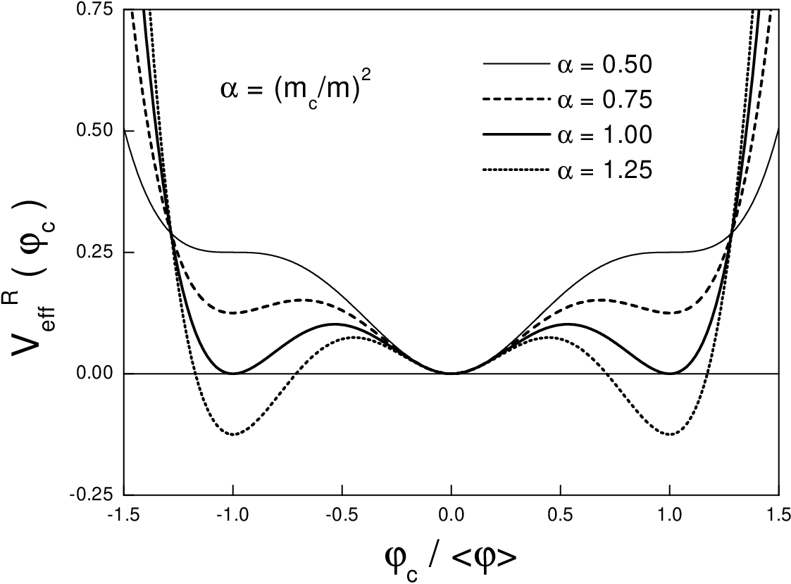
Let us examine how the energies of the different ground states that exchange stability at the critical mass $m_{c}$ behave in the neighborhood of the first order transition. For values of $m>m_{c}$, the stable ground state, i.e. the minimum of the effective potential, Eq. (4), occurs when the order parameter $\varphi_{c}=0$, such that, $V_{eff}(\varphi_{c}=0)=0$. The value of the effective potential at the metastable minimum $\varphi_{c}=\langle\varphi\rangle$ is given by,

$$V^{0}_{eff}(\langle\varphi\rangle)=\frac{1}{4}m^{2}\langle\varphi\rangle^{2}\left[1-\frac{m_{c}^{2}}{m^{2}}\right]$$

(6)

Then at $m^{2}=m_{c}^{2}$ the two ground states at ${\varphi_{c}=0}$ and $\varphi_{c}=\langle\varphi\rangle$ are degenerate and for $m^{2}<m_{c}^{2}$, the true ground state is at $\varphi_{c}=\langle\varphi\rangle$. The effective potential at $T=0$ represents the ground state energy [10] and close to the critical mass $m_{c}$, we find, $V_{eff}~\propto~|m^{2}-m_{c}^{2}|~\propto~|g|^{2-\alpha}$ which implies that the critical exponent $\alpha=1$ and if hyperscaling applies the correlation length exponent $\nu=1/{(d+z)}$. The latent heat is given by

$$L_{h}=(A_{+}+A_{-})=\frac{1}{4}m_{c}^{2}\langle\varphi\rangle^{2}$$

where we used $A_{+}=0$. Notice the existence of a spinodal at $(m_{c}/m)^{2}=0.5$ which marks the limit of metastability of the superconductor in the normal phase. On the other hand there is always a metastable minimum at $\varphi_{c}=0$ in the superconducting phase.

In order to treat the finite temperature case we note that for quantum theories of Euclidean fields at finite temperatures, the effective potential is equivalent to the thermodynamic free energy [10]. The generalization of the effective potential to $T\neq 0$ is done replacing frequency integrations in the calculation of the effective potential by a sum over Matsubara frequencies. The effective potential at finite $T$ ($k_{B}=1$) is given by,

	$\displaystyle V_{eff}(T)$	$\displaystyle=$	$\displaystyle\frac{1}{4}m^{2}\langle\varphi\rangle^{2}|g|\left\{1+\right.$		(7)
			$\displaystyle+\!\!\left.\frac{2}{\pi^{2}m^{2}\langle\varphi\rangle^{2}}\frac{T^{d+1}}{|g|}I\left(\frac{M(\varphi_{c})}{T}\right)\right\}$

where $M^{2}(\varphi_{c})=m^{2}+q^{2}\varphi_{c}^{2}$ and

$$I_{d}(y)=\int_{0}^{\infty}dxx^{d-1}\ln[1-e^{-\sqrt{x^{2}+y^{2}}}].$$

The function $I_{3}(y)=I(y)$ for three dimensions is plotted in the inset of Fig. 2. In the limit $T\gg M$ and close to the critical point, we have [3],

	$\displaystyle V_{eff}(\varphi_{c},T)=-\frac{\pi^{2}}{18}T^{4}-\frac{1}{8}m^{2}T^{2}+\frac{1}{2}m_{T}^{2}\varphi_{c}^{2}$
	$\displaystyle+\frac{\lambda}{24}\varphi_{c}^{4}+\frac{3q^{4}}{64\pi^{2}}\varphi_{c}^{4}[\ln(\frac{\varphi_{c}^{2}}{\Lambda^{2}})-\frac{25}{6}]$		(8)

where we defined a renormalized temperature dependent mass,

$$m_{T}^{2}=|m^{2}|(1-T^{2}/T_{MF}^{2})$$

with ${T_{MF}^{2}\approx 12|m^{2}|/3q^{2}}$. Alternatively we can write $m_{T}$ as

$$m_{T}^{2}=m^{2}+(q^{2}/4)T^{2}$$

(9)

and if we choose the arbitrary value of the quantity $\Lambda$ as the minimum, $\langle\varphi\rangle$, of the temperature dependent effective potential, we obtain

	$\displaystyle V_{eff}(\varphi_{c},T)=-\frac{\pi^{2}}{18}T^{4}-\frac{1}{8}m^{2}T^{2}+\frac{1}{2}m_{T}^{2}\varphi_{c}^{2}$
	$\displaystyle-\frac{m_{T}^{2}}{4\langle\varphi\rangle^{2}}\varphi_{c}^{4}+\frac{3q^{4}}{64\pi^{2}}\varphi_{c}^{4}[\ln(\frac{\varphi_{c}^{2}}{\langle\varphi\rangle^{2}})-\frac{1}{2}]$		(10)

Let us now discuss these results. First, notice from Eq. (9) that the line at which the temperature dependent mass $m_{T}$ vanishes is given by,

$$T_{MF}=\frac{2}{q}|m^{2}|^{1/2}$$

If we consider the contribution of terms of $O(\lambda)$, this temperature is in fact given by, ${T_{MF}^{2}=12|m^{2}|/(4\lambda+3q^{2})}$. This line has no special meaning since, on cooling the system a first order transition occurs before it, as we show below (see Fig. 2). It is governed by the same (mean-field) shift exponent, $\psi=z/(d+z-2)=1/2$, of the critical line of a neutral superfluid given by $T_{SF}^{2}=12|m^{2}|/(4\lambda)$. Notice that in the $3d$-case, this superfluid insulator transition at zero temperature is described exactly by the one-loop effective potential since $d+z=d_{c}=4$ is the upper critical dimension for this transition. This transition is the interaction driven quantum superfluid-insulator transition studied by Fisher et al. [11]. The insulating character of the disordered phase is due to the presence of a gap for excitations, $\Delta=|m^{2}|^{\nu z}=|m^{2}|^{1/2}$ since the correlation exponent $\nu$ assumes it’s mean-field value for $d=d_{c}$.

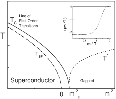
In the charged superfluid the actual transitions are quite different and occur for

$$m_{T}^{2}=m^{2}+(q^{2}/4)T_{c}^{2}=m_{c}^{2}$$

(11)

where $m_{c}^{2}$ is given by Eq. (5). The critical line of first order transitions is now given by,

$$T_{c}=\frac{2}{q}\sqrt{m_{c}^{2}-m^{2}}$$

(12)

and at the quantum critical point of the neutral superfluid, $m^{2}=0$, there is now a superconducting instability at a finite critical temperature,

$$T_{c}(m^{2}=0)=\sqrt{\frac{3}{8\pi^{2}}}q\langle\varphi\rangle$$

The physical origin of this phase transition is the energy gained by the system with the expulsion of the electromagnetic field when the system becomes superconducting.

From the temperature dependent effective potential of Eq. (7) and the plot of the function $I(y)$ in the inset of Fig. 2 we conclude that there are two relevant scales for the present problem in the disordered phase ($\varphi_{c}=0$, $m^{2}>m_{c}^{2}$). For $m/T\gg 1$, the thermal contribution to the effective potential vanishes exponentially as can be easily checked. For $m/T<0.12$, which corresponds to high temperatures $I(y)$ saturates, $I(y<0.12)\approx-2.16$. In this case the effective potential,

$\displaystyle V_{eff}(T)\approx\frac{1}{4}m^{2}\langle\varphi\rangle^{2}|g|\bigg\{1-\frac{4.32}{\pi^{2}m^{2}\langle\varphi\rangle^{2}}\frac{T^{d+1}}{|g|}\bigg\}$

which can be cast in the scaling form,

$$V_{eff}(T)\propto|g|^{2-\alpha}F\left[\frac{T}{T^{*}}\right]$$

with the critical exponent $\alpha=1$ and the characteristic temperature,

$$T^{*}\propto|g|^{\frac{z}{d+z}}=|g|^{\frac{1}{d+1}}=|g|^{\frac{1}{4}}.$$

This is similar to that of continuous quantum phase transitions, where $T^{*}\propto|g|^{\nu z}$ [3] but with $\nu=1/(d+z)$ confirming the expectations of our previous discussion. Notice that in the present problem, the mass $m$ (or $m^{2}$), the control parameter itself, provides the natural cut-off for breakdown of scaling along the temperature axis. The two characteristic energies $T^{*}$ and $m^{2}$, the scaling temperature and the cut-off scale are general features expected to play a role near quantum discontinuous transitions.

The quantum mechanical problem of two coexisting phases at $m_{c}$, the superconductor and the insulator, can be described by a double wave function $\psi=a\psi_{1}+b\psi_{2}$. In the probability density $|\psi|^{2}a^{2}|\psi_{1}|^{2}+b^{2}|\psi_{2}|^{2}+ab(\psi_{1}\psi_{2}^{*}+\psi_{2}\psi_{1}^{*})$, the coefficients $a^{2}$ and $b^{2}$ are the relative proportions of each phase. The interference term may have experimental significance as one of the phases has macroscopic coherence. Even if the overlap between the wave functions vanishes in the thermodynamic limit, at the first order transition it may give rise to finite corrections as the system is made up of finite domains due to the avoided criticality.

The transition investigated above is a special case of quantum first order transitions referred as fluctuation induced first order transitions. From the scaling analysis we expect however that the result $\nu=1/(d+z)$ holds generally for transitions with a latent heat. As an example that this is the case we investigate the biquadratic spin-1 chain [12],

$$H=-\sum_{i}\epsilon_{i}(\vec{S}_{i}\cdot\vec{S}_{i+1})^{2}$$

(13)

with

$$\epsilon_{i}=\left\{\begin{array}[]{ll}1&\mbox{if $i$ is odd}\\ \lambda&\mbox{if $i$ is even}\end{array}\right.$$

(14)

At $\lambda=1$ there is a zero temperature first order phase transition where two spontaneously dimerized ground states exchange stability [12]. The ground state energy can be written as

$$E_{g}(\lambda)-E_{g}(\lambda=1)=A_{\pm}|1-\lambda|$$

(15)

consistent with $\alpha=1$ and the latent heat ${L=-(A_{+}+A_{-})}$ can be exactly obtained [12]. Furthermore in this case the correlation length exponent has been directly obtained from finite lattice calculations [13]. The numerical value, $\nu\approx 0.5$ agrees with the expected value $\nu=1/(d+z)=1/2$ since for this transition $z=1$ [13].

The effects of disorder on classical first order transitions have been extensively studied [14]. Here we must distinguish weak or fluctuation-induced first order transitions from strong first order transitions which map into the random field problem [14] since disorder couples to the order parameter. In the latter case a criterion for the role of disorder based on domain wall arguments can be easily generalized to quantum systems. In analogy with the random field problem [15], we define a generalized stiffness $J$ associated with the (continuous) symmetry-broken phase [3], which scales as $J^{\prime}=b^{d+z-2}J$ close to the strong coupling attractor of this phase. In this equation $b$ is the scaling factor and $d$ and $z$ are respectively the dimension and the dynamical critical exponent discussed earlier. At this fixed point the random field scales as $h^{\prime}=b^{d/2}h$ [15], and their ratio

$$\left(\frac{h}{J}\right)^{\prime}=b^{\frac{4-(d+2z)}{2}}\left(\frac{h}{J}\right)$$

(16)

If $d+2z>4$ the fixed point at $(h/J)=0$ is stable and a critical amount of disorder is required to destroy the ordered phase. As concerns the first order transition this implies that the coexistence of phases is possible at least for sufficiently weak disorder. In the opposite case, i.e., for $d+2z<4$ disorder destroys the first order character of the transition since there can be no coexistence and one phase grows at the expenses of the other. The case $d+2z=4$ is marginal and requires specific calculations. For the biquadratic chain discussed above $d+2z=1+2=3<4$ and any amount of disorder drives this system to a random singlet phase associated with an infinite disorder fixed point as has been shown using a perturbative renormalization group calculation [16].

In the case of fluctuation induced quantum first order transitions we find no general criterion as for the standard case. For the problem treated here of a superconductor coupled to a gauge field, Boyanovsky and Cardy [17] have shown that to order $4-\epsilon$, at least for weak disorder, this transition remains first order.

We have investigated quantum first order transitions using scaling ideas and looking at two specific cases. In both cases there is a discontinuity in the first derivative of the ground state energy equivalent to a latent heat associated with the transition. Therefore, as in classical transitions, we have $\alpha=1$ which allows the definition of the correlation length exponent $\nu=1/(d+z)$ for the quantum case. The consideration of the problem of the superconductor coupled to a gauge field has been important to clarify the meaning of a scaling approach in a system where criticality is avoided. We have studied the effects of disorder in these transitions in the case this couples to fluctuations of the order parameter. A simple criterion to determine if the first order nature of the quantum transition is modified by disorder is discussed.

References

- [1] M. A. Continentino, G. Japiassu and A. Troper, Phys. Rev. B39 , 9734 (1989); M.A. Continentino, Phys. Rev. B47 , 11587 (1993).
- [2] J. Hertz, Phys. Rev. B14, 1165 (1976).
- [3] M. A. Continentino, Quantum Scaling in Many Body Systems, World Scientific, Singapore, 2001.
- [4] B. Nienhuis and N. Nauenberg, Phys. Rev. Lett. 35, 477 (1975).
- [5] M. E. Fisher and A. N. Berker, Phys. Rev. B 26, 2507 (1982).
- [6] B. Nienhuis, A. N. Berker, E. K. Riedel, and M. Schick, Phys. Rev. Lett. 43, 737 (1979).
- [7] J. Sólyom and P. Pfeuty, Phys. Rev. B 24, 218 (1981); L. Turban and F. Igloi, Phys. Rev. B 66, 014440 (2002).
- [8] S. Coleman and E. Weinberg, Phys. Rev. D7, 1888 (1973); B. I. Halperin, T. C. Lubensky and S. Ma, Phys. Rev. Lett. 32, 292 (1974).
- [9] A.P.C. Malbouisson, F. S. Nogueira and N.F. Svaiter, Mod. Phys. Letts. A11, 749 (1996).
- [10] R. Jackiw, Phys. Rev. D9, 1686 (1973).
- [11] M. P. A. Fisher, P.B. Weichman, G. Grinstein and D. S. Fisher, Phys. Rev. B40, 546 (1989).
- [12] M. Barber and M T. Batchelor, Phys. Rev. B40, 4621 (1989).
- [13] J. Sólyom, Phys. Rev. B36, 8642 (1987).
- [14] see J. L. Cardy, Physica A263, 215 (1999) and references therein.
- [15] B. Boechat and M.A. Continentino, J. Phys: Condensed Matter, 2 , 5277 (1990).
- [16] B. Boechat, A. Saguia e M.A. Continentino, Sol. St. Comm. 98, 411 (1996).
- [17] D. Boyanovsky and J. L. Cardy, Phys. Rev. B25, 7058 (1982).