Particle In Cell Simulation of Combustion Synthesis of TiC Nanoparticles
Abstract
A coupled continuum-discrete numerical model is presented to study the synthesis of TiC nanosized aggregates during a self-propagating combustion synthesis (SHS) process. The overall model describes the transient of the basic mechanisms governing the SHS process in a two-dimensional micrometer size geometry system. At each time step, the continuum (micrometer scale) model computes the current temperature field according to the prescribed boundary conditions. The overall system domain is discretized with a desired number of uniform computational cells. Each cell contains a convenient number of computation particles which represent the actual particles mixture. The particle-in-cell (discrete) model maps the temperature field from the (continuum) cells to the respective internal particles. Depending on the temperature reached by the cell, the titanium particles may undergo a solid-liquid transformation. If the distance between the carbon particle and the liquid titanium particles is within a certain tolerance they will react and a TiC particle will be formed in the cell. Accordingly, the molecular dynamic method will update the location of all particles in the cell and the amount of transformation heat accounted by the cell will be entered into the source term of the (continuum) heat conduction equation. The new temperature distribution will progress depending on the cells which will time-by-time undergo the chemical reaction. As a demonstration of the effectiveness of the overall model some paradigmatic examples are shown.
1 Introduction
The self-propagating high-temperature synthesis process (SHS) [12] is a promising method employed for the synthesis of many advanced materials, such as ceramic, intermetallics, composites, etc. [13]. Usually the process applies to powders mixture which are conveniently homogenized and pressed in order to form a loosely compacted pellet. The SHS exploits the ability of certain materials mixture in producing high exothermic and self-sustaining reactions once ignited locally or uniformly. Ignition can be made by a laser beam, induction, resistance, radiant or a spark source. The exothermic reaction makes the temperature increase rapidly in the pellet, reaching and surpassing the combustion temperature. The resulting product are usually very pure and rather porous (about 50% of the theoretical density [13]). The final product composition and its morphology depend on [14]:
- i)
-
initial particles size and distribution, shape and purity;
- ii)
-
initial density of the reacting mixture;
- iii)
-
initial temperature of the reacting system;
- iv)
-
size of the sample and reactor configuration;
- v)
-
dilution of the reacting mixture with the final product.
Thus, the actual combustion process involves simultaneously
critical factors at both the particle (i.e. i) and the sample
scale (i.e. ii-v).
Typical advantages of the process are:
- •
high purity products;
- •
low equipment, operation and processing costs;
- •
extremely short processing times;
- •
possibility of forming unique metastable phases with improved properties as a result of the inherent strong non-equilibrium conditions (i.e. steep thermal gradients and high heating/cooling rates).
However, beside the above advantages, the rapidity of SHS and the complexity of involved concomitant physical and chemical phenomena, makes rather difficult the optimization of the process as well as that of the chemistry and the morphology of the final products. In addition, the strong exothermicity of the reaction may generate a combustion wave which passes through all the pellet by igniting abnormally the reaction thus stopping or making unstable the reaction.
It is therefore desirable the development of flexible predictive
simulation tools in order to give a significant step forward to
the progress of the SHS process.
In this study we focus our
attention to a specific Ti and C particles mixture system, in
order to obtain TiC particles. According to standard
classification, this powder system involves a solid-solid reaction
in the sense that no gas reactant contributes to the combustion.
Many studies have been carried out on the SHS synthesis of TiC as model material under both microgravity [17, 19] and normal gravity [10, 18] conditions, either experimentally [17, 19] and theoretically [10, 18]. This system is particularly convenient because Ti and C powders are not very expensive. In addition, the formation heat of TiC is very large (185 kJ/mol) and the melting point of the product is very high (3423 K) which make the reactions initiation rather easy and the product formation straightforward.
The study of this reacting system is complex because of the many processes involved e.g. the propagation of the combustion wave in the given granular system, the phase changes of the metallic component, the occurrence of the chemical reaction, the physical and mechanical interaction among the powders and the heat and mass transport in the system which implies strongly inhomogeneous properties.
We propose a discrete approach to model the kinetics of the reaction considering the thermal and the chemical evolution of a small portion of the system, thereby simulating the actual non uniformity of the mixture properties.
In the section II, we describe the physical phenomena we take into consideration in the modelling. Section III describes the numerical methods used to reproduce these physics processes at macroscopic and microscopic level and their relative coupling. Section IV presents results on the formation of nanoparticles during a typical combustion process.
2 Physical processes and mathematical model
During the SHS operation, the pellets are rapidly heated. Usually, a thermal wave precedes the combustion front, thus preheating the powder mixture ahead. Usually, the metallic constituent has to melt before reaction occurs [15]. Under this condition, the reactions is mainly controlled by the carbon diffusion in the liquid Ti.
The reaction scheme is
| (1) |
All the atoms and molecules, and in particular the composites of titanium carbide, are subjects to an interaction potential with all the other species and at the same time they are thermically perturbed by the Brownian motion. In consequence of these competing effects nanoparticles of TiC can be formed.
In the developed model the following steps are considered:
- a)
-
the solid-liquid transition of titanium;
- b)
-
the chemical reaction between the melted titanium and the graphitic carbon granules;
- c)
-
the interaction between clusters of different kinds of particles (Ti, C and TiC);
- d)
-
the formation of nano-sized aggregates of TiC.
Below we analyze in detail the three fundamental steps: phase change, chemical reaction, nanoparticle formation.
2.1 Heat transfer and phase change
In the solid-liquid transition the enthalpy of the system has to be taken into consideration. In figure 1 the curve of the enthalpy per unit of mass () as a function of the temperature is shown for titanium.

The function includes three continuous parts divided by two
discontinuity points (i.e. A and B) at the and
-liquid transition, which occur at
K and K. During melting or
transition it is necessary to supply an extra amount of enthalpy
to break the interatomic bonds between the atoms of the solid
metal ( kJ/kg and kJ/kg respectively).
The enthalpy versus temperature function for a mass is defined
as
| (2) |
The heat conduction equation for the system is given by [9]:
| (3) |
where is temperature, the energy source, the density, the specific heat at constant pressure and the thermal conductivity.
However, equation (3) it is not convenient in this form when is discontinuous. In this condition the presence of a heat flux does not modify the temperature in the volume where phase change is taking place and the eq. (3) can be replaced more conveniently by:
| (4) |
where is the specific heat flux (J/s) across its surface given by the standard Fourier law
| (5) |
2.2 Chemical reaction
As experiments suggest we assume that the chemical reaction occurs
when the Ti surrounding the C particles has melted, while the
carbon remains solid since its melting point, K, is
far higher temperature. Similarly the TiC being created
is solid since its melting temperature is K.
Due to the exothermicity of the reaction, the heat source in eq.
(3) is evaluated as
| (6) |
where is the mass of the TiC product and indicates the heat generated per unit of mass of product( kJ/kg [7]).
2.3 Nanoclusters interactions
After the reaction has taken place, the temperature of the system
is locally increased and the TiC product becomes dispersed in the
liquid Ti phase. Since the atomistic simulation of Ti, C and TiC
is computationally prohibitively expensive, we consider the
dynamics of clusters made of a large number of atoms. The behavior
of the clusters attemps to reproduce on the average that of the
single particles relatively to the phenomena we study.
The motion of the cluster is partly deterministic (due to the
interaction with the other clusters) and partly stochastic,
because of their Brownian motion.
For the particles and
the potential energy has the form [3]
| (7) |
where and . The parameter defines the strength of the pair interaction and defines a length scale [3]. The interaction is repulsive at close distance, and attractive at larger distance. A cut off is assumed, for numerical convenience, beyond a limiting separation . The corresponding Lennard-Jones force is and has the expression
| (8) |
The detailed motion of the clusters is described by the Langevin equation [8]
| (9) |
where is the cluster mass, v the velocity, a parameter depending on the liquid [8] and the Brownian random force acting on the cluster.
The motion of these clusters, and in particular that of the TiC clusters, can generate a phenomenon of coalescence in the form of very small aggregates of nano-metric sizes. Thus, starting from micro-sized reacting particles of carbon, we obtain nano-sized aggregates of TiC.
3 Numerical methods
The simulation of the processes described above and the discretization of the various mathematical models used to describe them requires to handle multiple length and time scales. The Brownian motion and the chemical reactions are much slower than the evolution of the temperature. The processes at the particle level (chemical reactions, motion) require a spatial resolution at the nanometer range, while the temperature field is characterized by micrometer scales and the overall system is on the centimeter scale.
To handle these multiple scales we have decided to focus our attention at the mesoscopic level, describing the evolution of only a portion of the complete system. Our domain is on the micrometer range and is treated at that level using a continuum model discretized with a finite volume (FV) method. However, we retain the physics at the nanometer range by resorting to two additional methods: we describe the nanometer physics using computational particles. The interactions among particles at the nanometer range are treated with the molecular dynamics (MD) approach, and the coupling between mesoscopic (micrometer) scales and nanometer scales is treated with the particle in cell (PIC) method. Figure 2 summarizes the approach.

This approach has the advantage to use the numerical approach most suitable for each phenomenon we consider but requires to handle multiple methods and algorithms and their mutual interaction. To this end we have applied a modular approach based on the object-oriented software paradigm.
3.1 Mesoscopic model
The heat transfer in a system with phase changes is described by
equation (3) coupled to equation (5). It
is a continuum model that involves a local energy balance. At each
point of the system the enthalpy content, which depends on the
local temperature and on the state of aggregation of the matter,
is known.
When a chemical reaction event occurs, the amount
of energy released is added to the local enthalpy
content as a source term in eq. (3). Consequently the
local temperature is increased. The TiC particles generated become
a part of the system.
The integration of (3) and (5) is the
obtained using a finite volume method on a two dimensional
cartesian domain of sizes , with a
boundary indicated by . This system is discretized using a
two dimensional uniform grid in the direction and with
cells of sizes and . We also defined a third
dimension of size which is used to dimensionalize all
quantities as in the physical system. The time is discretized in
time steps .
The discretized forms of eq.
(4) and (3) are applied to cells with
or without phase change respectively. To avoid numerical
instabilities we use an implicit scheme based on the Euler
algorithm.
- •
cells with no phase change
(10) - •
cells with phase change
(11) being the perimeter of the cell in which phase change is taking place. The heat flux is calculated by the discretized form of eq. (5):
(12) where is the thermal conductivity at the interface between the and the cells. Its value is given by
(13) Analogous expressions are valid for all other interfaces.
Upon computing the coefficients at the time level , the eqs. (10)-(13) become a linear system which is solved using the GMRES algorithm.
A new algorithm has been implemented to solve the problems arising from the non-linearity and discontinuity of the enthalpy function versus temperature, . In order to illustrate the approach, we consider for convenience solidification first, and then melting for a given cell of the system.
3.1.1 Solidification
For temperatures above , we use eq. (10) to advance the temperature for the cell at the temporal step , the corresponding enthalpy content for a generic cell is given by
| (14) |
We indicate with and () the enthalpies of a cell of titanium corresponding to the beginning and the end of the solidification respectively.
Solidification starts when for we have
| (15) |
and at subsequent time levels , the following condition holds:
| (16) |
In that case, eq. (10) is no longer appropriate and the enthalpy and the temperature are advanced using:
| (17) |
Finally, the solidification process is completed at the time step , when the following condition holds:
| (18) |
In this last instance, the temperature is advanced as
| (19) |
Later, solidification no longer occurs in the cell and, for time steps , the temperature is again computed using eq. (10) and the enthalpy is given by
| (20) |
3.1.2 Melting
In the case of melting, the system starts at a temperature below and eq. (10) governs the evolution of the temperature. Again the enthalpy is computed from
| (21) |
The process of solidification starts at the time step , when the following conditions are verified
| (22) |
Subsequently, for , enthalpy and temperature are calculated using
| (23) |
Solidification ends at the time step , when the condition below is verified
| (24) |
At the time step , the temperature is advanced as prescribed by conservation of energy:
| (25) |
Finally when melting is completed, for the temperature is advanced using eq. (10) and the enthalpy is given by
| (26) |
3.2 Coupling of mesoscopic and nanometer scale through PIC
The mesoscopic subdivision of the system is made using the grid of
cells described above. The cells are used to treat the heat
transfer in a melting or solidifying continuum media.
To study
the nanometer scale physics and the detail of the phenomena at
particle (i.e. nanometer) level, it is necessary to use a discrete
approach. Thus, the Particle In Cell method (PIC)
[2] has been adopted. This implies that the system is
subdivided in computational particles which physically represent a
cluster of atoms. Therefore the granules of carbon correspond to a
set of computational particles with the properties of the carbon
atoms. Similarly the Ti and the TiC are represented by
computational particles with the corresponding properties. Then
the cell properties are computed based on the particles properties
which change in time. This approach is particularly convenient in
the study of powder systems when the mass transfer and the heat
transport are closely coupled.
The two levels of description of the system permit us to map not only the thermophysical properties (, and ) from one level to the other, but also to map the field variables such as temperature and enthalpy. Thus the temperature and the enthalpy of a particle can be computed by knowing the corresponding values in the cells and viceversa.
The approach followed is summarized in Fig. 2. The
system is characterized by particles, each of volume
, and concurrently the same system can also be represented
by cells of volume .
Assuming an equal number of
particles per cell, , the initial volume of each particle
is given by
| (27) |
By introducing a system of logical coordinates as and , for a generic cell and particle we define the assignment function W as the function resulting from the tensor product between functions of first order in each direction:
| (28) |
where () is the position of the particle, () the position of the cell center and is given by
| (29) |
This function which will be denoted by
for shorthand, gives the contribution of a generic
property of the particle to the cell as a function of the
relative positions.
Similarly, it is possible to perform the opposite operation
consisting in mapping a property (or a physical quantity) of the
cells to a particle.
The properties and the physical quantities that are calculated with this method are summarized in Table I.
| From particles to cells | From cells to particles |
|---|---|
By knowing the temperature in each cell, at each time step it is possible to single out those where the reaction can take place. By recalling the basic assumption, e.g. the titanium must be melted before the reaction can take place, the condition that must be verified is
| (30) |
Another necessary condition in order to have a reaction in the cells which fulfil the condition (30), is that each cell contains at least one particle of titanium and one of carbon. If more than one couple is present, then the reaction occurs first between those particles which have the shortest distance. These two particles are thus replaced by two new ones. If we indicate with the particle of titanium and with that of carbon, the number of moles of the new TiC particle being created is
| (31) |
whereas its volume is
| (32) |
where and are the
molecular weights of titanium and carbon.
For sake of mass
balance a new particle must be introduced into the system. This
can be either C or Ti particle. Its volume must fulfils the
conditions (33)
| (33) |
If the condition is verified, only a particle of
TiC is created.
The amount of energy developed during the formation of the
TiC particle is calculated using eq. (6).
3.3 Molecular Dynamics treatment of nanometer scale particles
The interaction between different particles in the system and
among the atoms that compose them is an aspect which plays a very
important role in the phenomenon of the formation of
nanoparticles. This interaction is reproduced by the Lennard-Jones
potential. This is only a first approximation of the real
situation, because it usually holds for atoms or molecules and not
for clusters. Indeed, our computational particles represent
cluster of atoms that, on average, we assume interacting with a
potential that includes a repulsive and an attractive part as that
of Lennard-Jones. In calculating the potential we consider the
distance between the center of the clusters.
The equations of
the motion for a generic computational particle are
| (34) | |||||
| (35) |
where x, v and F are position, velocity and force for a particle of mass . The equations of motion are solved using the Verlet algorithm [1]. To simulate the stochastic behaviour due to the Brownian motion of the particle we use the Andersen thermostat approach [1]. We consider each cell as interacting with an heat bath which sets its temperature at the value given by the continuum model described above while, at the same time, it permits this subsystem to access all the energy shells corresponding to this temperature according to their Boltzmann weight [1]. The coupling of the system to the bath is represented by stochastic velocities which are occasionally randomly assigned to the computational particles, using a collision probability. The strength of this coupling depends on the frequency of stochastic collisions between particles. The values of the accessible velocities are those of the Maxwell-Boltzmann distribution [8] with variance
| (36) |
where is the Boltzmann constant and is the temperature of the particle.
4 Results of the simulations
4.1 Validation test - 1D analytical benchmark
At first, we performed a comparison between the results of the present model with an analytical solution for a system undergoing a phase change [9]. The simulation has been carried out on a one-dimensional domain of length made of titanium for a time with the following initial and boundary conditions
| (37) |
In fig. 3 we show the time evolution of the liquid-solid interface. As it is possibile to see the agreement with the analytical solution is good. We have conducted a convergence study to verify the correctness of the implementation of the heat transport algorithm described above.

4.2 Validation test - 2D phase change benchmark
We carried out a simulation for a two-dimensional system made of titanium with sizes for a time . The initial and boundary conditions were
| (38) |
The enthalpy versus the temperature for the central cell is shown in fig. 4. The result proves that the phase change happens correctly and with the correct enthalpy change corresponding to the latent heat.

4.3 Formation kinetics of TiC nanoparticles
In this case the system considered is composed by titanium
surrounding three granules of graphite, two with a diameter
and the other with diameter . The size
of each side of the domain is .
The properties of the materials, and in particular the specific
heat and the thermal conductivity, depend on the temperature and
are obtained from [4, 5]. The density is
assumed as constant for both materials and equal to that at
. This means that the effects of the volume variation of
the species during the process are neglected.
A generic heat source is introduced to simulate the melting of titanium. The thermal behavior of the system assumes the following initial and boundary conditions
| (39) |
The domain is subdivided by using and cells along and directions respectively and with particles per cell. The simulation time is , the numbers of time steps in the heat equation and in the motion equations are and respectively. Subcycling of the heat equation is used to handle its much faster scale, compared with the scale of the particle motion. For the simulation shown below, the following values were used: , , , , and . The initial velocity of all particles is zero, allowing the Andersen thermostat to establish the proper thermal equilibrium. The collision frequency used in the Andersen thermostat is .
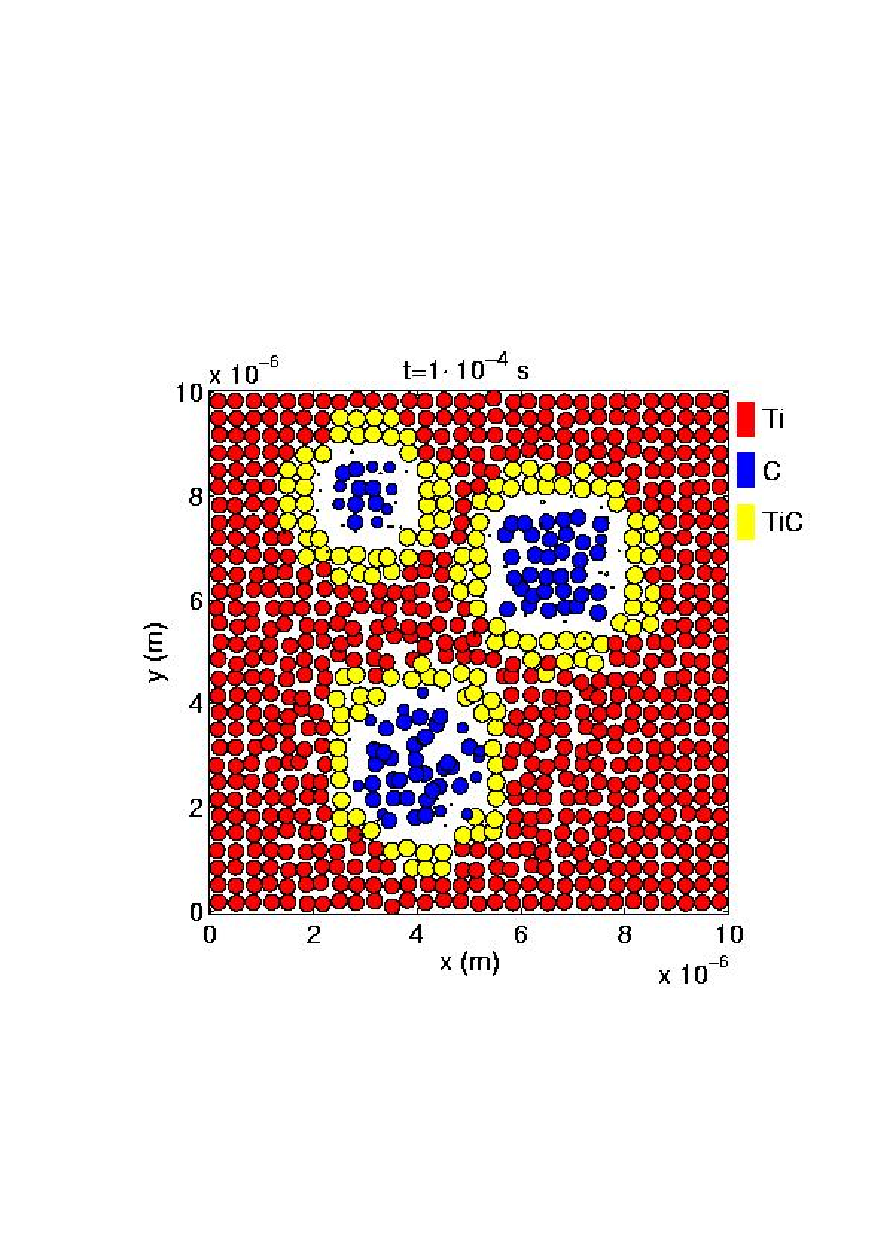
The time evolution of the reacting system is shown in fig. 5. The evolution of the combustion process is evident: TiC shells of particles are first formed at the interface between graphite and liquid Ti, as demonstrated in the experiments. After this stage, the thermal agitation of the particles breaks the shells and permits that the reaction develops further. The final aggregates of particles are the end product of the reaction: TiC nanoparticles.
 |
 |
 |
 |
Figure 6 shows the evolution of the concentration of the various chemical species for the same simulation.

5 Conclusions
A new coupled mesoscopic-nanometer scale model has been developed
to simulate the SHS process. The approach combines the solution of
PDEs for the continuum media on the mesoscopic level with the
discrete PIC-MD techniques for the nanometer scale. This model
permits the description of thermal phenomena on the mesoscale and
physical and chemical interaction on the nanoscale of both
reagents and products species.
The overall model offers a unique
opportunity to follow the evolution of the nanostructure during
the SHS process.
An interesting output of the meso/nano model is
the concentration history of chemical species which are relatively
easy accessible by actual experiments.
The model has been
validated against an analytical solution. The PIC-MD model
requires direct experimentation in order to determine the most
suitable LJ parameters and the collision frequency value
for more realistic application of the developed model.
Acknowledgments
This research is supported by the United States Department of Energy, under contract W-7405-ENG-36.
References
- [1] D. Frenkel, B. Smit, Understanding Molecular Simulation Academic Press, San Diego (1996).
- [2] R.W. Hockney, J.W. Eastwood, Computer simulation using particles A. Hilger, Bristol (1988).
- [3] D.C. Rapaport, The Art of Molecular Dynamics Simulation Cambridge Univ. Press, Cambridge (1995).
- [4] Y.S. Touloukian, D.P. DeWitt, Thermal Radiative Properties: Metallic Elements and Alloys IFI/Plenum, New York (1970).
- [5] Y.S. Touloukian, D.P. DeWitt, Thermal Radiative Properties: Nonmetallic Solids IFI/Plenum, New York (1970).
- [6] A.W. Weimer, Carbide, Nitride and Boride Synthesis and Processing Chapman and Hall, London (1997).
- [7] M.G. Lakshmikantha, J.A. Sekhar, Metallurgical Trans. A 24, 617 (1993).
- [8] F. Reif, Fundamentals of Statistical and Thermal Physics McGraw-Hill, New York (1965).
- [9] H.S. Carslaw, J.C. Jaeger, Conduction of Heat in Solids Oxford University Press, Oxford (1986).
- [10] A.M. Kanury, Metallurgical Trans. A 23, 2349 (1992).
- [11] A.G. Merzhanov, Combust. Sci. and Tech. 98, 307-336 (1994).
- [12] A.G. Merzhanov and I.P. Boroviskaya, Comb. Sci. and Tech. A 10, 175 (1975).
- [13] S.B. Badhuri and S. Badhuri, Combustion Synthesis in Non-equilibrium Processing of Materials C. Suryanarayama Ed., Pergamon Materials Series (1999).
- [14] A.W. Weiner, Carbide, Nitride and Boride Materials Synthesis and Processing, Chapman and Hall (1997).
- [15] S.D. Dunmead, D.W. Readey and C.E. Semler, J. Am. Cer. Soc. 72(12), 2318 (1989).
- [16] D.C. Halvenson, K.H. Ewald and Z. Munir, J. Mat. Sci. 28, 4583 (1993).
- [17] A. Makino, N. Araki, and T. Kuwabara, Trans. Jpn. Soc. Mech. Eng. B58(55), 271 (1992).
- [18] M.G. Lakshmikantha, A. Bhattacharya and J.A. Sekkar, Met. Trans. A23, 23 (1992).
- [19] Y. Tanabe, T. Sakamoto, N. Okada, T. Akatsu and E. Yasuda, J. Mat. Res. 14, 1516 (1999).