Weakly Interacting Bose Gas in the Vicinity of the Critical Point
Abstract
We consider a three-dimensional weakly interacting Bose gas in the fluctuation region (and its vicinity) of the normal-superfluid phase transition point. We establish relations between basic thermodynamic functions: density, , superfluid density , and condensate density, . Being universal for all weakly interacting systems, these relations are obtained from Monte Carlo simulations of the classical model on a lattice. Comparing with the mean-field results yields a quantitative estimate of the fluctuation region size. Away from the fluctuation region, on the superfluid side, all the data perfectly agree with the predictions of the quasicondensate mean field theory.—This demonstrates that the only effect of the leading above-the-mean-field corrections in the condensate based treatments is to replace the condensate density with the quasicondensate one in all local thermodynamic relations. Surprisingly, we find that a significant fraction of the density profile of a loosely trapped atomic gas might correspond to the fluctuation region.
pacs
03.75.Hh, 05.30.Jp, 67.40.-wI Introduction
Typically, only special properties of critical systems (such as critical exponents and amplitude ratios) are universal (see, e.g. Ref. book). Weakly interacting models, including dilute Bose gases (BG), are an exception from this rule in the sense that all their thermodynamic properties are universal close to the critical point. This unique feature allows complete characterization of the fluctuation region and its vicinity for all such models without adjustable parameters. In the recent paper our2D devoted to two dimensional systems we obtained the universal thermodynamic relations for the density, , superfluid density, , and quasicondensate density, , by performing high-precision Monte Carlo simulations of the classical model on a lattice. Here we present the results of a similar study of the three-dimensional (3D) case.
Away from the critical point, the mean-field (MF) treatment of the weakly interacting BG bogoliubov; LP; Popov is a reliable theoretical scheme controlled by the small dimensionless parameter
| (1) |
where is the scattering length. In the pseudo-potential approach, one models the same scattering length by introducing a weak short-range potential, , of radius and amplitude . The relation between and is provided by the perturbation theory (we set )
| (2) |
The divergence of the second term in the ultra-violet limit is cut at ; it cancels out when final answers are expressed in terms of the scattering length bogoliubov; LP; Popov. Close to the Bose condensation point, when , one can write Eq. (1) as
| (3) |
In the fluctuation region,
| (4) |
( is the critical temperature), perturbative in approaches do not work Popov; Baym99; Baym00; AM2000; us; AM. The physics now is determined by non-perturbative coupling between the long-wavelength components of the order parameter field, resulting in a crossover from MF to the generic U(1)-universality class critical behavior on approaching the critical point.
An important observation about the fluctuation region of a weakly interacting BG is that in the small interaction limit all models—quantum or classical, continuous or discrete—allow a universal description Popov; Baym99; our2D. The crucial circumstance is that long-wavelength components of the order parameter field, , with momenta much smaller then the thermal momentum are classical in nature (large occupation numbers), and only components with are strongly coupled. In this limit the effective Hamiltonian is given by the classical model
| (5) |
where is the renormalized chemical potential for long-wave modes. The microscopic physics of different models is important only at momenta , where the system behavior is perturbative and thus may be easily accounted for analytically.
Our approach to the problem starts from observation that , , and , are universal functions of the shifted chemical potential, , where are the (model specific) critical point parameters. To find these functions one has to solve accurately any of the weakly interacting models, and we resort to Monte Carlo (MC) simulations of the classical model on a lattice using very efficient Worm-algorithm not suffering from the critical slowing down Worm. In 2D, the same idea was successfully implemented in Ref. our2D. Before that, quantum to classical mapping was used in Refs. us; AM; PRS to determine the critical point parameters (both in 2D and 3D).
This approximation-free numerical solution yields an accurate description of the system thermodynamics. In the critical region, characterized by known exponents of the U(1) universality class, our goal is to find amplitudes of the power-law dependencies for all quantities in question. By comparing to the results of the MF theory, we establish quantitative limits on the size of the fluctuation region. Away from the fluctuation region our accurate data unambiguously distinguish between MF theories based on the notion of condensate and quasicondensate—the amplitude of the order parameter field at intermediate distances—in favor of the latter.
In the past, most non-perturbative calculations using renormalization group (RG) and -expansions (for the most recent work see, e.g., Refs. stoof; Baym00; AM2000; kleinert; Kastening; ledowski) concentrated on the critical temperature shift, , and the scattering in the results was quite substantial. In the absence of small parameters controlling the accuracy of the answer, the knowledge of final results is crucial in discriminating between competing approaches and in developing better schemes. However , or , is only one of many universal properties of weakly interacting systems. The critical chemical potential shift as well as superfluid and condensate density behavior in the critical regime are also universal. A reliable theoretical approach should be able to reproduce all of them, and our results provide corresponding benchmarks.
The paper is organized as follows. In Sec. II we use the analysis of dimensions to cast thermodynamic relations for the weakly interacting gas in the universal form. Special attention is paid to the ultra-violet and infra-red procedures of the chemical potential renormalization. In Sec. III we render MF theory based on the quasicondensate density. In Sec. IV we introduce the classical model on a lattice and the simulation algorithm. Our results are presented and compared to the critical and MF behavior in Secs. V. In Sec. VI we discuss our results in the context of experiments with ultracold gases and make comparisons with some analytical approaches to the fluctuation region.
II Universal relations for weakly interacting models
In the limit one can present simple arguments for the typical energy and density scales responsible for the non-perturbative behavior at the critical point Baym99; us; AM. To find the momentum separating weakly and strongly coupled modes, , one considers the three terms in the Hamiltonian (5) and determines when all of them are of the same order of magnitude for modes , assuming that modes with are already taken into account in renormalized values of the Hamiltonian parameters. This leads to the estimates
| (6) |
where
| (7) |
is the long wavelength contribution to the total density, and is the effective chemical potential for low-energy modes. In 3D one has , and since is separating strongly coupled long-wave harmonics from slightly perturbed short-wave ones, the order-of-magnitude estimate for may be obtained from the ideal system formula:
| (8) |
Substituting this back to Eqs. (6)-(7) yields
| (9) |

The critical values of the density, or chemical potential, are, of course, model specific. [We find it convenient to work in the grand canonical ensemble and keep temperature fixed; in Sec. V we explain how all the results are easily converted into more familiar temperature plots.] In fact, in 3D the major contribution to , and , is coming from high momenta . However, this model specific contribution to density does not depend on interactions in linear order in U, and thus can be easily calculated analytically. Thus if we count density and chemical potential from their critical values, we expect the dependence of on to be universal because of its long-wavelength nature. In view of Eq. (9) we write the equation of state in the dimensionless form as
| (10) |
where is the universal control parameter
| (11) |
with the typical variation across the fluctuation region of order unity. [For the gas in a slowly varying external potential, , the function describes the spatial density profile, provided in Eq. (11) is replaced with .] Similarly,
| (12) |
| (13) |
Establishing universal—for all weakly-interacting models—functions , , and , and explaining how they work for the quantum Bose gas is the main goal of this paper.
First, we note that and for the Bose gas have been already determined in previous MC studies us; AM; AM2002. The interaction induced shift of the critical density is universal
| (14) |
where is the critical density of the non-interacting system; for the Bose gas. [We quote the mean of the results presented in Refs. us and AM which overlap within the error bars.]
Before quoting the result for , we would like to discuss its subtle structure AM; Baym2001; AM2002. Linear in terms are accounted for by the MF expression . There are two distinctive contributions to which are quadratic in . One is universal and comes from strongly coupled critical fluctuations. The other one is perturbative and comes from the second-order diagram (see Fig. 1) for the self-energy, :
| (15) | |||||
where is the dispersion law, is the Matsubara frequency, and is the Bose distribution function. The corresponding classical expression is obtained by considering only the zero-frequency term ():
| (16) |
The self-energy integrals are divergent. In the infrared limit the divergence is logarithmic
| (17) |
For the Bose gas () it is also divergent in the ultra-violet limit as a power law
| (18) |
We cast the last expression in the form which immediately relates it to the definition of the pseudo-potential, Eq. (2), i.e. in the sum the ultra-violet divergences cancel each other for terms . Identically, the same result is obtained if in all final answers we simply substitute and use
| (19) |
as the second-order self-energy for the quantum Bose gas. In what follows we employ this well established trick bogoliubov; LP; Popov. Obviously, in classical models quantum corrections to are absent. Correspondingly, there are no divergencies in apart from the logarithmic one, and the original expression for the self-energy should be used: .
The logarithmic divergence (17) can be simply truncated at some infra-red energy scale, or regularized AM; AM2002. Whatever the procedure, as long as it is the same for all weakly-interacting models, the difference between the true value of and is coming from long-wave modes and thus is universal, while the term is model specific. In this paper we introduce an explicit infra-red cutoff by adding a constant to the dispersion law, i.e. everywhere in Eqs. (15) and (16). Then
| (20) |
The numerical value of has been determined in Refs. AM; AM2002. For the quantum gas it reads
| (21) |
where
| (22) |
In the MF theory, the definition of the effective chemical potential involves subtraction of the self-energy contributions
| (23) |
This quantity is model-independent, and we find it convenient to introduce the corresponding universal function
| (24) |
It is, of course, directly related to the equation of state function
| (25) |
If we were to change the infra-red cutoff in the definition of self-energy, we would have to modify the value of accordingly .
III Mean-field Theory
Away from the fluctuation region our simulation is supposed to reproduce the known perturbative results for a weakly interacting Bose gas. That is we need , , , and as functions of , the dimensionless variable playing the role of the small parameter that guarantees the applicability of perturbative treatment. The leading terms in the perturbative expansion away from the fluctuation region are , the next-order terms are . We confine ourselves to considering only these terms, ignoring the higher order corrections (in fact, we are not aware of existing results for them). Hence, our numerics is expected to agree with the known analytic results only at large enough , and only up to some constants.
This degree of accuracy can be achieved within the MF treatment (plus an extra care of the higher-energy logarithmic correction to the chemical potential) both on the normal and superfluid sides. In the superfluid region, however, it is essential, that MF be based on the quasicondensate, rather than genuine condensate. In the condensate-based treatments the same accuracy is achieved only if beyond-the-MF corrections are taken into account. The logarithmic correction to the chemical potential, , has been already discussed in Sec. II. For practical purposes, this correction is not large—unless the gas parameter is exponentially small, and taking it into account really makes sense only if all the -independent terms are accounted for as well. Theoretically, however, this correction involves the ultraviolet physics and thus is model-specific. Hence, if we ignore it, then we cannot render our answers model-independent. On the good side, we do not need to calculate more accurately than it was done in Sec. II, since that would lead to the higher-order corrections which we ignore here. Thus, we simply add the term (20) to MF expression for the chemical potential of the Bose gas.
III.1 Asymptotic behavior in the normal phase ()
In the normal region we have and identically zero. Hence, the only quantity we have to look at is the equation of state or . Using MF equation for the effective chemical potential , we calculate the difference between the density of the interacting gas and the critical density of the ideal gas keeping only the leading linear in terms:
| (26) |
We now notice that , see Eqs. (10) and (14), and use Eq. (25) to complete the derivation
| (27) |
III.2 Mean-field description of the superfluid region (). Quasicondensate
The standard MF approach to the weakly interacting Bose gas deals with the condensate density, , defined through the one-particle density matrix,
| (28) |
[ is either the field operator (in the quantum system) or a complex valued field (in the classical system); in the latter case ], as
| (29) |
Well inside the region of applicability of the MF description, but not too far from the fluctuation region, the MF theory based on is less accurate than the theory dealing with the notion of quasi-condensate. Of course one can go beyond the MF description in the condensate based theory and evaluate the corresponding corrections. It is important, however, that the quasicondensate MF description automatically captures the first order corrections to the condensate MF. [In 2D the quasicondensate MF has demonstrated perfect agreement with MC simulations away from the fluctuation regionour2D.] We thus find it instructive to resort here to the quasicondensate MF description.
The notion of quasicondensate was introduced by PopovPopov (“bare condensate” in the original version). Basically, it is used to describe the order parameter with fluctuating phase (see also KSS) and implies the possibility of parameterizing the field for the weakly interacting system as
| (30) | |||||
| (31) |
where is the quasicondensate density, and is the Gaussian field independent of . The Gaussian field is primarily responsible for the decay of at distances comparable to the thermal wavelength. The relation between and immediately follows from (30)-(31):
| (32) |
When fluctuations of the phase field, , become noticeable—this is precisely the case in the vicinity of the critical point— the difference between and should be taken into consideration as well.
There are strong arguments that it is , and not , that is relevant to all the characteristics of the system, with being just one of them. Indeed, the physics at large distances, or small, but finite momenta, including the spectrum of elementary excitations, is determined by what is happening on smaller lengthscales, in other words, “high-energy” physics ultimately determines what happens at lower energies. The condensate is the macroscopic characteristic of the system; it should be derived from other finite- properties, and governs them.
This fact has been rigorously shown by one of us Svist. Though the analysis of Ref. Svist has been done for 2D systems (where the notion of quasicondensate is of crucial importance and cannot be avoided), it is applicable to the 3D case as well. The actual treatment closely follows Popov’s theory Popov, with the only (but important) exception that is understood and treated as a physical quantity. [Popov treated bare condensate as an auxiliary mathematical quantity explicitly dependent on the momentum separating ‘slow’ harmonics from the ‘fast’ ones. Correspondingly, he attempted to exclude this quantity from final answers to render them -independent.—At low enough temperatures this can be easily done by replacing . However, in the high temperature region the quantity is a meaningful physical parameter KSS.]
One may consider Eq. (31) as the definition —it is the modulus of the order parameter field at large distances. This quantity appears in all MF equations just like does at low temperature. Then, and can be chosen as convenient independent thermodynamic parameters specifying the state of the system, the rest of the characteristics being expressed as functions of . The basic results are as follows KSS; Svist:
| (33) |
with the non-quasicondensate part of the particle density, , given by the integral
| (34) |
where is the free-particle dispersion law, and
| (35) |
is the Bogoliubov quasiparticle spectrum.
For the one-particle density matrix one obtains Svist (see also Ref. Krasavin for a numeric check in 2D)
| (36) |
| (37) |
| (38) |
[In Eq. (38), as well as in Eq. (34), the first term in square brackets is after integration, and may be omitted in the region addressed in the present paper.]
That is the relevant quantity behind the long-wave physics is clear from the structure of Eqs. (36)-(38). The second term in Eq. (38) decays first as a power law , and then exponentially fast, so that on large length-scales the amplitude of the order parameter is given by . Phase fluctuations are described by . They are negligible at short distances of order , but at distances their contribution to the density matrix results in the difference between and , see Eq. (32):
| (39) |
The trick to solve MF equations in the vicinity of the critical point () is to calculate differences between the corresponding densities (this makes all integrals to converge at energies ) keeping only the universal leading low-momenta terms. To get we add and subtract the ideal gas critical density
| (40) |
where
| (41) |
is the dimensionless parameter of asymptotic expansion for all thermodynamic quantities away from the fluctuation region.
The relation for the condensate density immediately follows from the asymptotic value of the phase correlator
| (44) |
Hence
| (45) |
To find , we consider the standard expression for the normal component density LP
| (46) |
Integrating by parts, we rewrite Eq. (46) as
| (47) |
We now subtract from the non-condensate density to evaluate the integral explicitly, and use identity to get
| (48) |
Finally, the quasicondensate density can be related to the chemical potential as KSS
| (49) |
where we have added the term , in accordance with the previous discussion. In contrast to the analogous relation in terms of the condensate and non-condensate densitiesHP, this relation does not imply corrections of the order .
Comparing Eq. (49) with the definition of -function, Eq. (24), we see that
| (50) |
and with the – relation (25) and Eq. (43) for we get a self-consistent equation for
| (51) |
Equation (51) along with Eqs. (50), (43), (45), and (48) define , , , and as functions of .
We are in a position now to demonstrate that quasicondensate MF reproduces results of the condensate-based diagrammatic technique which accounts for leading, , corrections to the condensate MF answers Popov. Indeed, in the limit , Eqs. (51) and (45) define the effective chemical potential dependence on the condensate density as
| (52) |
Similarly,
| (53) |
in complete agreement with Ref. Popov.



IV Lattice model and simulation algorithm
As explained in Secs. I and II, one can introduce universal functions for any model described in the long-wave limit by the Hamiltonian (5) with small . Classical lattice models are easier to deal with numerically, and there are very efficient classical algorithms which allow simulations of very large system sizes. In the present study, we performed simulations of systems with up to lattice points. In addition, results obtained for a classical model directly test the idea of universality, since they have to agree with all MF predictions formally derived for the quantum Bose gas.
Our simulations were done for the simple cubic lattice Hamiltonian
| (54) |
where is the Fourier transform of the complex lattice field , and
| (55) |
is the tight-binding dispersion law with momentum confined within the first Brillouin zone (BZ). The self-energy expression (16) was evaluated with this dispersion law and numerically for each system size, and used then in the definition of the function , Eq. (24).
We employed the Worm algorithm for classical statistical systems Worm which has Monte Carlo estimators for all quantities of interest here and does not suffer from critical slowing down. In cluster methods Wolff (which have comparable efficiency) the calculation of the superfluid density is more elaborate.
From simulations of a series of system sizes and coupling constants, , we eliminated finite-size and finite- corrections to the final results for , , , and .
V Simulation results
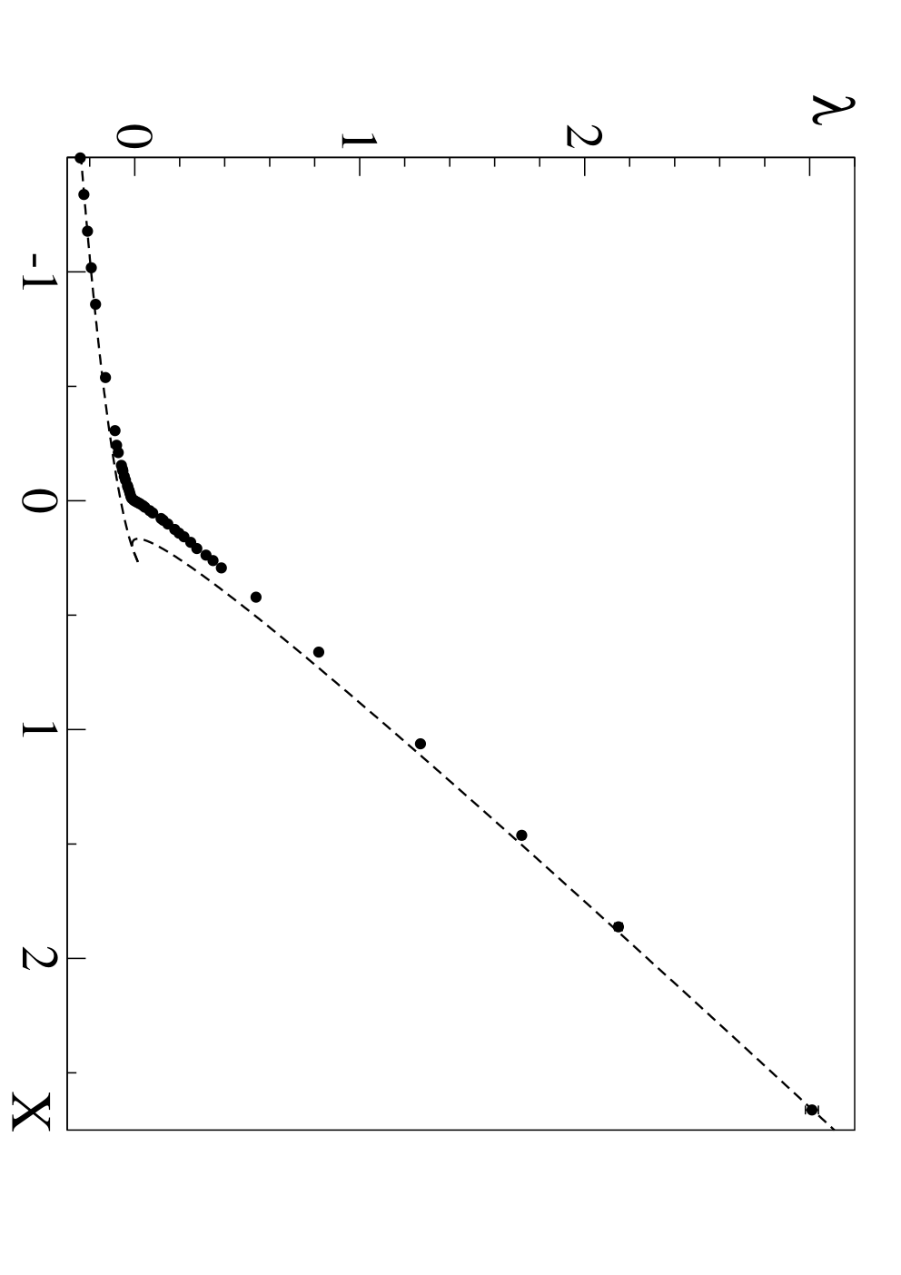
In Figs. 2 and 3 we present the final outcome of simulations throughout the fluctuation region. We also present all the data in Table I. The relative accuracy is high far from the fluctuation region (better then ), and gets worse in the vicinity of the critical point where finite-size corrections are the largest. We show errorbars in all plots.
First, we check for consistency between our approach and the previously obtained result for , see Eq. (22). Within the errorbars, the agreement is perfect, see Fig. 4.
Knowing and is all we need to address the asymptotic MF behavior at large , see Eqs. (51), (42), (45), and (48). The agreement with the MF theory based on the notion of quasicondensate is remarkable. Despite the fact that in MF we keep consistently only large terms and , for numeric reasons the constant term also happens to be accurate. The self-consistent theory of Ref. BH is claimed to go beyond conventional MF, but it is not known at present whether it reproduces correctly the terms.
The agreement between the data and MF predictions makes it easy to estimate the size of the fluctuation region (in terms of ) to be about on the superfluid side of the transition, and roughly two times smaller, , on the normal side.
Other quantities of interest are the universal amplitudes for the superfluid and condensate densities in the critical regime, when , and . Here and are the correlation length and the correlation function critical exponents of the XY-universality class in , see, e.g., Ref. Campostrini. By fitting the data for and at small to the power laws with known exponents we obtain
| (56) |
| (57) |
-effect. It appears in Fig. (2) as if the total density has a cusp at the critical point. However, is not singular at , and what looks as a cusp in Fig. (2) is in fact a relatively sharp crossover slightly shifted to the normal side of the transition point, see Fig. (4).
The crossover itself is predicted by MF equations since changes its slope from roughly to , see Eqs. (27) and (51). We are not aware of any special reason why it has to be so sharp and so close to the transition point—the slope changes at and the crossover region is only about in width. We call this surprising non-perturbative result the “-effect” as suggested by the shape of the -function.


VI Discussion
To discuss results in the canonical ensemble setup we need to change from the chemical potential as a control variable to reduced temperature. First, we note that our results immediately generalize to the case when the properly rescaled reduced density
| (58) |
is used as a tuning variable. Indeed,
| (59) |
is nothing but the parametric dependence of the condensate density on density at a fixed temperature [and similarly for and ].


Next, we observe that Eq. (14) can be also considered as an equation for
| (60) |
Using it in the definition of the -function we obtain
Finally, keeping only the leading linear in and terms we arrive at
| (61) |
where is the rescaled reduced temperature parameter
| (62) |
This establishes the functional relation between and , and the parametric dependence of other properties on .
In Figs. 5 and 6 we plot , and dependencies on the reduced temperature variable . From Fig. 5 we deduce the size of the fluctuation region consistent with the previous estimate in terms of and relation , i.e. it is about on the superfluid side and on the normal side. Amazingly, in temperature plots for and one may not even distinguish between the MF theory and numerical data on large scale; only in the inset which covers just the fluctuation region we can see that the MF curve goes wrong very close to .
We also verify the prediction of the self-consistent theory BH for the critical amplitude of the condensate density. As mentioned previously, the self-consistent theory makes predictions for the critical region as well; the relation between the condensate density and reduced temperature is derived as [see Eq. (18) in Ref. BH] with . The condensate density exponent is accurate, though the derivation was done assuming that the self-energy behaves as instead of the true critical behavior with (see Ref. Campostrini and the discussion below). Since the amplitude in the critical law is directly related to the value of in Eq. (57)
| (63) |
in disagreement with the theory by a factor of two.
To characterize the fluctuation region in terms of the gas parameter we identically rewrite
| (64) |
The coefficient in the denominator is too large to be ignored even in qualitative estimates. It was mentioned in Ref. us that Bose gases should demonstrate universal properties only at . This statement is unambiguously confirmed by the present study, since for larger values of the fluctuation region in temperature is already of order itself. The other identical way of writing is
| (65) |
Obviously, the idea of universality is meaningful only if it is possible to separate ideal-gas short-wavelength physics from strongly coupled long-wavelength fluctuations, i.e. when , and thus, according to Eq. (65), the fluctuation region in reduced temperature is small.
In a typical experiment with ultracold gases the parameter is as small as , and the system may be considered as weakly interacting. The interaction induced critical temperature shift in the homogeneous system is very small (the corresponding critical density shift is given by Eq. (14) and is only about 1% for ) and is difficult to study experimentally. This does not imply, however, that all non-perturbative effects in the vicinity of the critical point are of academic interest as well.
The quantity directly relevant to the experimental setup is since it describes, according to Eq. (10), the density profile in the trapping potential if it is smooth enough to guarantee the hydrostatic regime. In this regime the density variation over the mode-coupling radius reduces to , where is the homogeneous equation of state, , and is the trapping potential. It follows from Figs. 2 and 4 that the “cusp” on the density profile does not coincide with the point where the condensate first appears, but is slightly shifted to the perimeter of the trap. Moreover, by fitting experimental data away from the “cusp” using MF equations, one may directly measure the interaction induced universal chemical potential shift [through ].
The variation of the -function across the fluctuation region is about , which transforms into density variation of order
| (66) |
or a strong effect for ! In Fig. 7 we show the density profile in a smooth parabolic trap
| (67) |
when the condensate density in the middle of the trap is comparable to the critical density. Amazingly, in this situation the fluctuation region extends all the way from the critical point to the trap center, and the MF theory completely fails to describe the superfluid side. Thus, the non-perturbative physics of the fluctuation region and the prediction that it is completely characterized by the classical field theory can be studied even by experimenting with very dilute gases, . As Fig. 7 clearly demonstrates, all effects in the middle of the trap are strong.
It is also worth mentioning that in the fluctuation region the density profile can not be decomposed into the sum of the smoothly varying, monotonic non-condensate density background and the condensate density bump. The normalized condensate density in Fig. 7 increases faster then , and the naive “decomposition” technique would underestimate the actual condensate density by almost a factor of two.
For the quasi-homogenenous description to work, it is necessary to keep the external potential gradients small. If the chemical potential in the middle of the trap corresponds to , then the critical point is located at a distance . The hydrostatic approach can be used when , or
| (68) |
For the parameters in Fig. 7 we need then — a condition easily satisfied experimentally gasreview. The crucial point is then in achieving the necessary spatial resolution in shallow traps.


Our final result concerns the universal part of the self-energy at the critical point Baym00; BH; ledowski. The most recent calculation based on renormalization group equations for the vertex functions ledowski predicted ():
| (69) |
with , , and an extended crossover between the free particle and critical regimes (we preserve the present paper definition of ).
This quantity is directly related to the occupation numbers in the limit by . In Worm algorithms, the one-particle density matrix is calculated automatically as the central part of the numerical scheme Worm, and thus is readily available. In Fig. 8 we plot the universal part of the occupation number distribution as versus (in the inset we plot versus , i.e. subtracting the leading bare spectrum dependence) for the system size and see the crossover between the free particle, , and the U(1) critical, , behavior at . The smallest values of are effected by finite size effects and are not shown in the inset (in finite systems is finite at the critical point).
The correlation function exponent is known very accurately Campostrini , and we consider it as known (our data are consistent with this value). Clearly, very little changes occur in the structure of the expression across the fluctuation region. It seems the best way to characterize the crossover is to write the whole expression as with interpolating between and . Also, the crossover is localized in the vicinity of . The numerical value of in the asymptotic limit is found to be very close to unity
| (70) |
VII Acknowledgments
This work was supported by NASA under grant NAG32870. B.S. acknowledges a support from the Netherlands Organization for Scientific Research (NWO).
| -3.738 | 3.17 | -0.406(1) | ||
| -3.338 | 2.82 | -0.381 | ||
| -2.938 | 2.47 | -0.355 | ||
| -2.538 | 2.13 | -0.327 | ||
| -2.138 | 1.79 | -0.297(1) | ||
| -1.738 | 1.45 | -0.263 | ||
| -1.498 | 1.26 | -0.242 | ||
| -1.338 | 1.13 | -0.226 | ||
| -1.178 | 1.00 | -0.210(1) | ||
| -1.018 | 0.874 | -0.193 | ||
| -0.8584 | 0.751 | -0.174 | ||
| -0.5384 | 0.517 | -0.130(1) | ||
| -0.3064 | 0.361 | -0.0875(3) | ||
| -0.2424 | 0.323 | -0.0804(2) | ||
| -0.2104 | 0.304 | -0.0732(4) | ||
| -0.1544 | 0.275 | -0.0593(6) | ||
| -0.1384 | 0.267 | -0.0546(7) | ||
| -0.1304 | 0.263 | -0.0527(2) | ||
| -0.1064 | 0.252 | -0.0462(3) | ||
| -0.09039 | 0.246 | -0.0409(3) | ||
| -0.06639 | 0.237 | -0.0324(5) | ||
| -0.05839 | 0.234 | -0.0299(6) | ||
| -0.04479 | 0.229 | -0.0251(7) | ||
| -0.03199 | 0.227 | -0.0213(12) | ||
| -0.01839 | 0.225 | -0.0173(11) | ||
| -0.01039 | 0.226 | -0.0134(7) | ||
| -0.002393 | 0.235(1) | -0.0046(18) | ||
| 0.001607 | 0.244(2) | 0.0021(15) | 0.0116(30) | 0.0130(30) |
| 0.005607 | 0.255(2) | 0.0094(18) | 0.0240(15) | 0.0259(16) |
| 0.009607 | 0.266(2) | 0.0171(11) | 0.0356(10) | 0.0381(11) |
| 0.01361 | 0.277(1) | 0.0243(8) | 0.0446(7) | 0.0482(8) |
| 0.02161 | 0.294(3) | 0.0367(23) | 0.0630(6) | 0.0674(7) |
| 0.02850 | 0.307(2) | 0.0456(8) | 0.0772(8) | 0.0826(8) |
| 0.04350 | 0.332(2) | 0.0663(8) | 0.105(1) | 0.111(1) |
| 0.05361 | 0.349(1) | 0.0802(21) | 0.123 | 0.132 |
| 0.07761 | 0.394(2) | 0.117(3) | 0.160(2) | 0.173(2) |
| 0.08561 | 0.406(1) | 0.127(2) | 0.173(1) | 0.187(2) |
| 0.1016 | 0.431(1) | 0.147(4) | 0.197(2) | 0.215(1) |
| 0.1256 | 0.469(1) | 0.178(3) | 0.237(4) | 0.255(3) |
| 0.1416 | 0.492(2) | 0.197(4) | 0.260(2) | 0.279(3) |
| 0.1576 | 0.518(2) | 0.219(3) | 0.287(4) | 0.310(6) |
| 0.1816 | 0.555(1) | 0.249(2) | 0.320(3) | 0.342(4) |
| 0.2089 | 0.587(8) | 0.276(4) | 0.360(8) | 0.386(5) |
| 0.2376 | 0.637(3) | 0.317(4) | 0.401(4) | 0.426(9) |
| 0.2616 | 0.672(3) | 0.348(5) | 0.434(5) | 0.462(4) |
| 0.2936 | 0.716(2) | 0.385(3) | 0.479(2) | 0.511(6) |
| 0.4216 | 0.895(2) | 0.539(3) | 0.652(3) | 0.683(7) |
| 0.6616 | 1.21(1) | 0.818(9) | 0.956(7) | 0.995(10) |
| 1.062 | 1.72 | 1.27(1) | 1.44(1) | 1.51(1) |
| 1.462 | 2.22(1) | 1.72(1) | 1.93(1) | 2.00(2) |
| 1.862 | 2.69(1) | 2.15(2) | 2.40(1) | 2.47(3) |
| 2.662 | 3.63(2) | 3.01(3) | 3.28(4) | 3.39(7) |
| 3.462 | 4.56(3) | 3.89(4) | 4.20(3) | 4.33(5) |
References
- (1) J. Zinn-Justin, Quantum Field Theory and Critical Phenomena, 3-d ed., Clarendon Press, Oxford (1996).
- (2) N. Prokof’ev and B.V. Svistunov, Phys. Rev. A 66, 043608 (2002).
- (3) N. Bogoliubov, J. Phys. USSR 11, 23 (1947).
- (4) E.M. Lifshitz and L.P. Pitaevskii, Statistical Physics, Part II, Pergamon, (1980).
- (5) V.N. Popov, Functional Integrals in Quantum Field Theory and Statistical Phisics, Reidel, Dordrecht, (1983).
- (6) G. Baym, J.-P. Blaizot, M. Holzmann, F. Laloë, and D. Vautherin, Phys. Rev. Lett. 83, 1703 (1999).
- (7) G. Baym, J.-P. Blaizot, and J. Zinn-Justin, Europhys. Lett. 49, 150 (2000).
- (8) P. Arnold and B. Tomik, Phys. Rev. A 62, 063604 (2000).
- (9) V. A. Kashurnikov, N.V. Prokof ev, and B.V. Svistunov, Phys. Rev. Lett. 87, 120402 (2001).
- (10) P. Arnold and G. Moore, Phys. Rev. Lett. 87, 120401 (2001); Phys. Rev. E 64, 066113 (2001).
- (11) N.V. Prokof’ev, and B.V. Svistunov, Phys. Rev. Lett. 87, 160601 (2001).
- (12) N. Prokof’ev, O. Ruebenacker, and B. Svistunov, Phys. Rev. Lett. 87, 270402 (2001).
- (13) H.T.C. Stoof, Phys. Rev. A 45, 8398 (1992); M. Bijlsma and H.T.C. Stoof, Phys. Rev. A 54, 5085 (1996).
- (14) H. Kleinert, cond-mat/0210162.
- (15) B. Kastening, cond-mat/0303486; cond-mat/0309060.
- (16) S. Ledowski, N. hasselmann, and P. Kopietz, cond-mat/0311043.
- (17) P. Arnold, G. Moore, and B. Tomik, Phys. Rev. A 65, 013606 (2002).
- (18) M. Holzmann, G. Baym, J.-P. Blaizot, and F. Lalo, Phys. Rev. Lett. 87, 120403 (2001).
- (19) Yu. Kagan, B.V. Svistunov, and G.V. Shlyapnikov, Sov. Phys. - JETP 66, 314 (1987).
- (20) B.V. Svistunov, Ph. D. Thesis, Kurchatov Institute, Moscow, 1990.
- (21) Yu. Kagan, V.A. Kashurnikov, A.V. Krasavin, N.V. Prokof’ev, and B.V. Svistunov, Phys. Rev. A 61, 43608 (2000).
- (22) N.M. Hugenholtz and D. Pines, Phys. Rev. 116, 489 (1959).
- (23) U. Wolff, Phys. Rev. Lett. 62, 361 (1989).
- (24) M. Holzmann and G. Baym, Phys. Rev. Lett. 90, 040402 (2003).
- (25) M. Campostrini, M. Hasenbusch, A. Pelissetto, P. Rossi, and E. Vicari, Phys. Rev. B 63, 214503 (2001).
- (26) F. Dalfovo, S. Giorgini, L.P. Pitaevskii, and S. Stringari, Rev. Mod. Phys. 71, 463 (1999).