Optical properties of polaronic excitons in stacked quantum dots

V. N. Gladilin, S. N. Klimin, V. M. Fomin, and J. T. Devreese Affiliation: Theoretische Fysica van de Vaste Stoffen, Departement Natuurkunde, Universiteit Antwerpen, Universiteitsplein 1, B-2610 Antwerpen, Belgium

August 11, 2026

Abstract

We present a theoretical investigation of the optical properties of polaronic excitons in stacked self-assembled quantum dots, which is based on the non-adiabatic approach. A parallelepiped-shaped quantum dot is considered as a model for a self-assembled quantum dot in a stack. The exciton-phonon interaction is taken into account for all phonon modes specific for these quantum dots (bulk-like, half-space and interface phonons). We show that the coupling between stacked quantum dots can lead to a strong enhancement of the optical absorption in the spectral ranges characteristic for phonon satellites.

pacs

78.67.Hc,73.21.La,73.21.-b

Non-adiabaticity is an inherent property of exciton-phonon systems in various quantum-dot structures. Non-adiabaticity drastically enhances the efficiency of the exciton-phonon interaction. The effects of non-adiabaticity are important to interpret the surprisingly high intensities of the phonon ‘sidebands’ observed in the optical absorption, the photoluminescence and the Raman spectra of quantum dots, in particular, an enhancement of these intensities with decreasing the quantum-dot size (see, e. g., Refs. JH96; cap2000). Deviations of intensities of the phonon-peak sidebands, observed in some experimental optical spectra, from the Franck-Condon progression, which is prescribed by the commonly used adiabatic approximation, find a natural explanation within our non-adiabatic approach 12; nanot; PSS03; raman2002. Recently, stacked quantum dots have received increasing attention (see, e. g., Refs. Schmidt97; Luyken99; NN1; pi01; Bayer01; NN4; NN5) due to the possibility to finely control their energy spectra. This makes stacked quantum dots very promising for future nanodevices NN4; NN5. In the present work, the non-adiabatic approach is applied to stacked InAs/GaAs quantum dots, which reveal a richer structure of phonon and exciton spectra in comparison with those for a single quantum dot.

In order to model coupled self-assembled InAs/GaAs quantum dots, we consider a stack of $N$ parallelepiped-shaped quantum dots with sizes $l_{x},$ $l_{y},$ $l_{z}$ and interdot distance $d$ along the $z$ -axis. Within the present approach, the lateral sizes ( $l_{x},$ $l_{y}$ ) of each quantum dot in a stack are supposed to be much larger than its size $l_{z}$ along the growth axis. The stack is a system of $\left(2N+1\right)$ layers ( $n=1,\ldots 2N+1$ ) with parameters

\left\{\begin{array}[c]{ll}l_{n}=l_{z},\;\varepsilon_{n}=\varepsilon_{\mathrm{InAs}}&\mathrm{for}\;n=2,4,\ldots,2N;\\ l_{n}=d,\;\varepsilon_{n}=\varepsilon_{\mathrm{GaAs}}&\mathrm{for}\;n=3,5,\ldots,2N-1;\\ l_{n}\rightarrow\infty,\;\varepsilon_{n}=\varepsilon_{\mathrm{GaAs}}&\mathrm{for}\;n=1,2N+1.\end{array}\right.

The bulk-like optical-phonon frequencies in InAs and GaAs layers of the stacked InAs/GaAs quantum dots coincide with the LO-phonon frequencies in InAs and GaAs, respectively. The interface frequencies belong to the stacked quantum dots as a whole and satisfy the dispersion equation

\det\left\|a_{kn}\left(\omega\right)\right\|=0\quad\left(k,n=1,\ldots 2N\right),

(1)

where $a_{kn}\left(\omega\right)$ is the dynamic matrix of the interface vibrations with the matrix elements

\left\{\begin{array}[c]{l}a_{nn}\left(\omega\right)=\varepsilon_{n}\left(\omega\right)\coth q_{\parallel}l_{n}+\varepsilon_{n+1}\left(\omega\right)\coth q_{\parallel}l_{n+1},\\ a_{n,n-1}\left(\omega\right)=a_{n-1,n}\left(\omega\right)=-\varepsilon_{n}\left(\omega\right)/\sinh q_{\parallel}l_{n};\end{array}\right.

(2)

all other matrix elements are equal to zero.

In Fig. 1, typical interface-phonon spectra are represented for stacked InAs/GaAs quantum dots formed by two InAs parallelepipeds. The frequencies are plotted as a function of the in-plane wave number $q_{\parallel}$ , which takes discrete values due to the quantization of the phonons in the $xy$ -plane. In a stack of $N$ quantum dots, each interface-phonon frequency of a single quantum dot splits into $N$ branches. The splitting of the interface-phonon frequencies is due to the electrostatic interaction between the optical polar vibrations of the different quantum dots.

These features of the optical-phonon spectrum of stacked quantum dots are manifested in their optical properties. We calculate the optical absorption spectrum of polaronic excitons in stacked quantum dots starting from the Kubo formula. Within the non-adiabatic approach 12 the following expression results for the linear coefficient of the optical absorption by the exciton-phonon system in a quantum-dot structure:

\alpha(\Omega)\propto\mbox{Re}\sum\limits_{\beta,\beta^{\prime}}d_{\beta}^{*}d_{\beta^{\prime}}\int\limits_{0}^{\infty}dt\,e^{i(\Omega-\Omega_{\beta}+i0^{+})t}\left\langle\beta\left|\bar{U}(t)\right|\beta^{\prime}\right\rangle,

(3)

where $\Omega$ is the frequency of the incident light, $d_{\beta}$ and $\Omega_{\beta}$ are, respectively, the electric dipole matrix element and the Franck-Condon frequency of a transition between the exciton vacuum state and the one-exciton state $|\beta\rangle$ . Exciton states in stacked InAs/GaAs quantum dots are determined using an exact diagonalization of the exciton Hamiltonian with simple parabolic valence and conduction bands within a finite-dimensional basis of the electron-hole states. The evolution operator averaged over the phonon ensemble, $\bar{U}(t)$ , is

	$\displaystyle\bar{U}(t)$	$\displaystyle=\mathrm{T}\exp\Biggl\{-\frac{1}{\hbar^{2}}\sum\limits_{\lambda}\int\limits_{0}^{t}dt_{1}\int\limits_{0}^{t_{1}}dt_{2}\left[\frac{\mbox{e}^{-i\omega_{\lambda}\left(t_{1}-t_{2}\right)}}{1-y_{\lambda}}\right.\Biggr.$
		$\displaystyle\Biggl.\left.\times\gamma_{\lambda}(t_{1})\gamma^{{\dagger}}_{\lambda}(t_{2})+\frac{y_{\lambda}\mbox{e}^{i\omega_{\lambda}\left(t_{1}-t_{2}\right)}}{1-y_{\lambda}}\gamma^{{\dagger}}_{\lambda}(t_{1})\gamma_{\lambda}(t_{2})\right]\Biggr\}.$		(4)

In Eq. (4), $\mathrm{T}$ is the time ordering operator, the index $\lambda$ labels the phonon modes specific for the quantum-dot structure under consideration, $\omega_{\lambda}$ are phonon frequencies, $\gamma_{\lambda}(t)$ are the exciton-phonon interaction amplitudes in the interaction representation, and $y_{\lambda}=\mbox{exp}\left(-\hbar\omega_{\lambda}/k_{B}T\right)$ .

Within the adiabatic approximation, which has been widely used to calculate the optical spectra of quantum dots, non-diagonal matrix elements of the exciton-phonon interaction are neglected when calculating $\alpha(\Omega)$ as given by Eq. (3) with Eq. (4). In the adiabatic approach 8; 9 one supposes that (i) both the initial and the final states of a quantum transition are non-degenerate, (ii) the energy differences between the exciton states are much larger than the phonon energies. It has been shown in Refs. 12; nanot; PSS03; raman2002 that these conditions are often violated for optical transitions in small quantum dots, which have sizes less than the bulk exciton radius. In other words, the exciton-phonon system in a quantum dot can be essentially non-adiabatic. The polaron interaction for an exciton in a degenerate state results in internal non-adiabaticity (“the proper Jahn–Teller effect”), while the existence of exciton levels separated by an energy comparable with the LO-phonon energy leads to external non-adiabaticity (“the pseudo Jahn–Teller effect”).

In Ref. 12, a method was proposed to calculate the absorption spectrum given by Eqs. (3) and (4) taking into account the effect of non-adiabaticity on the probabilities of phonon-assisted optical transitions. The key step is the calculation of the matrix elements of the evolution operator $\langle\beta\left|\bar{U}(t)\right|\beta^{\prime}\rangle$ . In order to describe the effect of non-adiabaticity both on the intensities and on the positions of the absorption peaks, a diagrammatic approach can be used. When calculating these matrix elements we take into account that in a quantum dot, due to the absence of momentum conservation, the product $\langle\beta_{1}|\gamma_{\lambda}|\beta_{2}\rangle\langle\beta_{2}|\gamma_{\lambda}^{*}|\beta_{3}\rangle$ can be non-zero for $\beta_{1}\neq\beta_{3}$ , as distinct from the bulk case. Consequently, the evolution operator is in general non-diagonal in the basis of one-exciton wavefunctions $|\beta\rangle$ . For the absorption coefficient we obtain

	$\displaystyle\alpha(\Omega)$	$\displaystyle\propto-{\rm Im}\sum\limits_{\beta}\|d_{\beta}\|^{2}G_{\beta}\left(\Omega+i0^{+}\right)-{\rm Im}\sum\limits_{\beta,\beta^{\prime}}d_{\beta}d^{*}_{\beta^{\prime}}$
		$\displaystyle\times\left[Q^{(1)}_{\beta\beta^{\prime}}(\Omega+i0^{+})+Q^{(2)}_{\beta\beta^{\prime}}(\Omega+i0^{+})\right],$		(5)

where

\displaystyle G_{\beta}\left(\Omega\right)

\displaystyle=\sum\limits_{\{j_{\lambda}=-\infty\}}^{\{\infty\}}\frac{C_{\{j_{\lambda}\}\beta}^{(+)}}{A_{\beta}\left(\Omega-\sum\limits_{\lambda}j_{\lambda}\omega_{\lambda}\right)},

(6)

\displaystyle A_{\beta}\left(\Omega\right)=\Omega-\Omega_{\beta}+\sum\limits_{\lambda}S_{\lambda,\beta}\omega_{\lambda}-\Sigma_{\beta}^{(1)}\left(\Omega\right)-\Sigma_{\beta}^{(2)}\left(\Omega\right),

(7)

	$\displaystyle C_{\{j_{\lambda}\}\beta}^{(\pm)}$	$\displaystyle=\prod\limits_{\lambda}(\pm 1)^{j_{\lambda}}{\rm exp}\left[\mp(2\bar{n}_{\lambda}+1)S_{\lambda\beta}+\frac{j_{\lambda}\hbar\omega_{\lambda}}{2k_{B}T}\right]$
		$\displaystyle\times I_{\|j_{\lambda}\|}\left({S_{\lambda\beta}}\left[2\sinh\left(\frac{\hbar\omega_{\lambda}}{2k_{B}T}\right)\right]^{-1}\right).$		(8)

$I_{n}(x)$ is a modified Bessel function of the first kind and $S_{\lambda\beta}$ is the Huang-Rhys parameter, which is related to the interaction of the exciton in the state $\beta$ with phonons of the $\lambda$ -th mode:

\displaystyle S_{\lambda\beta}=\left|\frac{\langle\beta|\gamma_{\lambda}|\beta\rangle}{\hbar\omega_{\lambda}}\right|^{2}.

(9)

The self-energy terms $\Sigma_{\beta}^{(1)}\left(\Omega\right)$ and $\Sigma_{\beta}^{(2)}\left(\Omega\right)$ in Eq. (7) are obtained by summing diagrams, which describe one- and two-phonon non-adiabatic contributions:

\displaystyle\Sigma_{\beta}^{(1)}\left(\Omega\right)=\sum\limits_{j=\pm 1}\sum\limits_{\lambda,\beta_{1}}F_{\beta\beta_{1}}\left(\Omega-j\omega_{\lambda}\right)M_{\lambda\beta\beta_{1}\beta_{1}\beta}^{(j)}

(10)

and

$\displaystyle\Sigma_{\beta}^{(2)}\left(\Omega\right)$	$\displaystyle=\sum\limits_{j_{1},j_{2}=\pm 1}\sum\limits_{\lambda_{1},\lambda_{2}}\sum\limits_{\beta_{1},\beta_{2},\beta_{3}}F_{\beta\beta_{1}}\left(\Omega-j_{1}\omega_{\lambda_{1}}\right)$
	$\displaystyle\times F_{\beta\beta_{3}}\left(\Omega-j_{2}\omega_{\lambda_{2}}\right)\left[F_{\beta\beta_{2}}\left(\Omega-j_{1}\omega_{\lambda_{1}}-j_{2}\omega_{\lambda_{2}}\right)\phantom{M_{\lambda_{2}\beta_{1}\beta_{2}\beta_{3}\beta}^{(j_{2})}}\right.$
	$\displaystyle\times M_{\lambda_{1}\beta\beta_{1}\beta_{2}\beta_{3}}^{(j_{1})}M_{\lambda_{2}\beta_{1}\beta_{2}\beta_{3}\beta}^{(j_{2})}+F_{\beta\beta_{2}}\left(\Omega\right)$
	$\displaystyle\times\left.M_{\lambda_{1}\beta\beta_{1}\beta_{1}\beta_{2}}^{(j_{1})}M_{\lambda_{2}\beta_{2}\beta_{3}\beta_{3}\beta}^{(j_{2})}\left(1-\delta_{\beta_{2}\beta}\right)\right]$	(11)

where

F_{\beta\beta_{1}}\left(\Omega\right)=\sum\limits_{\{j_{\lambda}=-\infty\}}^{\{\infty\}}C_{\{j_{\lambda}\}\beta}^{(-)}G_{\beta_{1}}\left(\Omega-\sum\limits_{\lambda}j_{\lambda}\omega_{\lambda}\right),

(12)

\displaystyle M_{\lambda\beta_{1}\beta_{2}\beta_{3}\beta_{4}}^{(j)}=m_{\lambda\beta_{1}\beta_{2}\beta_{3}\beta_{4}}^{(j)}-m_{\lambda\beta_{1}\beta_{1}\beta_{1}\beta_{1}}^{(j)}\delta_{\beta_{1}\beta_{2}}\delta_{\beta_{3}\beta_{4}},

(13)

\displaystyle m_{\lambda\beta_{1}\beta_{2}\beta_{3}\beta_{4}}^{(j)}=\frac{j\langle\beta_{2-j}|\gamma_{\lambda}|\beta_{3-j}\rangle\langle\beta_{2+j}|\gamma_{\lambda}^{{\dagger}}|\beta_{3+j}\rangle}{\hbar^{2}\left(1-y_{\lambda}^{j}\right)}.

(14)

The functions $Q^{(1)}_{\beta\beta^{\prime}}(\Omega)$ and $Q^{(2)}_{\beta\beta^{\prime}}(\Omega)$ in Eq. (5), which describe contributions of one- and two-phonon processes to non-diagonal matrix elements of the evolution operator, take the form

	$\displaystyle Q^{(1)}_{\beta\beta^{\prime}}(\Omega)$	$\displaystyle=G_{\beta}\left(\Omega\right)G_{\beta^{\prime}}\left(\Omega\right)\left(1-\delta_{\beta\beta^{\prime}}\right)$
		$\displaystyle\times\sum\limits_{j=\pm 1}\sum\limits_{\lambda,\beta_{1}}G_{\beta_{1}}\left(\Omega-j\omega_{\lambda}\right)m_{\lambda\beta\beta_{1}\beta_{1}\beta^{\prime}}^{(j)},$		(15)

$\displaystyle Q^{(2)}_{\beta\beta^{\prime}}(\Omega)$	$\displaystyle=G_{\beta}\left(\Omega\right)G_{\beta^{\prime}}\left(\Omega\right)\left(1-\delta_{\beta\beta^{\prime}}\right)$
	$\displaystyle\times\sum\limits_{j_{1},j_{2}=\pm 1}\sum\limits_{\lambda_{1},\lambda_{2}}\sum\limits_{\beta_{1},\beta_{2},\beta_{3}}G_{\beta_{1}}\left(\Omega-j_{1}\omega_{\lambda_{1}}\right)$
	$\displaystyle\times G_{\beta_{3}}\left(\Omega-j_{2}\omega_{\lambda_{2}}\right)\left\{G_{\beta_{2}}\left(\Omega-j_{1}\omega_{\lambda_{1}}-j_{2}\omega_{\lambda_{2}}\right)\phantom{M_{\lambda_{2}\beta_{1}\beta_{2}\beta_{3}\beta}^{(j_{2})}}\right.$
	$\displaystyle\times\left[\left(1-\delta_{\beta_{3}\beta_{1}}\right)m_{\lambda_{1}\beta\beta_{1}\beta_{3}\beta^{\prime}}^{(j_{1})}m_{\lambda_{2}\beta_{1}\beta_{2}\beta_{2}\beta_{3}}^{(j_{2})}\right.$
	$\displaystyle+\left.m_{\lambda_{1}\beta\beta_{1}\beta_{2}\beta_{3}}^{(j_{1})}m_{\lambda_{2}\beta_{1}\beta_{2}\beta_{3}\beta^{\prime}}^{(j_{2})}\right]+G_{\beta_{2}}\left(\Omega\right)\left(1-\delta_{\beta_{2}\beta}\right)$
	$\displaystyle\times\left.\left(1-\delta_{\beta_{2}\beta^{\prime}}\right)m_{\lambda_{1}\beta\beta_{1}\beta_{1}\beta_{2}}^{(j_{1})}m_{\lambda_{2}\beta_{2}\beta_{3}\beta_{3}\beta^{\prime}}^{(j_{2})}.\right\}$	(16)

The absorption spectrum is thus expressed through the functions $G_{\beta}\left(\Omega\right)$ , which in turn are determined by a closed set of equations (6), (7), and (10) to (12).

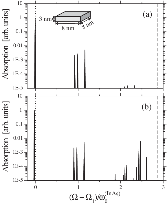
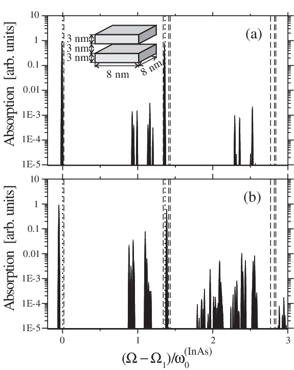
In Figs. 2 and 3 the calculated optical absorption spectra are shown for a single quantum dot and for a system of two stacked quantum dots, respectively. The calculations where performed for low temperatures ( $\left\{y_{\lambda}\ll 1\right\}$ ) when the absorption-line broadening due to the exciton-LO-phonon interaction is negligible. The broadening shown in Figs. 2 and 3 is introduced only to enhance visualization. From the comparison of the spectra obtained in the adiabatic approximation with those resulting from the non-adiabatic approach, the following effects of non-adiabaticity are revealed. First, the polaron shift of the zero-phonon lines with respect to the bare-exciton levels is larger in the non-adiabatic approach than in the adiabatic approximation. Second, there is a strong increase of the intensities of the phonon satellites compared to those given by the adiabatic approximation. This increase can be by more than two orders of magnitude. Third, in the optical absorption spectra found within the non-adiabatic approach, there appear phonon satellites related to non-active bare exciton states.

Fourth, the optical-absorption spectra demonstrate the crucial role of non-adiabatic mixing of different exciton and phonon states in quantum dots. This results in a rich structure of the absorption spectrum of the exciton-phonon system GBFD2001; nanot; PSS03. For the stacked quantum dots, this effect is enhanced in the (quasi-) resonant case, when the exciton-level splitting, caused by the coupling between quantum dots, is close to a LO phonon energy [see panel (b) in Fig. 3]. Similar conclusions about the influence of the exciton-phonon interaction on the optical spectra of quantum dots have been recently formulated in Ref. VFB2002 for the “strong coupling regime” for excitons and LO phonons. Such a “strong coupling regime” is a particular case of the non-adiabatic mixing related to a (quasi-) resonance, which arises when the spacing between exciton levels is close to the LO phonon energy.

In some cases (see, e. g., Ref. 12) the luminescence spectrum of a quantum dot can be easily derived from its absorption spectrum. E. g., under the assumption that the distribution function of the states of an exciton coupled to the phonon field, $f(\Omega)$ , depends only on the energy of a state, the luminescence intensity at low temperatures ( $\left\{y_{\lambda}\ll 1\right\}$ ) can be represented as

	$\displaystyle I(\Omega)$	$\displaystyle\propto\sum\limits_{K=0}^{\infty}\frac{1}{K!}\sum\limits_{\lambda_{1},\ldots,\lambda_{K}}f\left(\Omega+\sum\limits_{k=0}^{K}\omega_{\lambda_{k}}\right)$
		$\displaystyle\times\left.\left(\prod\limits_{k=1}^{K}\frac{\partial}{\partial y_{\lambda_{k}}}\right)\alpha(\Omega)\right\|_{\{y_{\lambda}\rightarrow 0\}}.$		(17)

Equation (17) is applicable, for instance, for thermodynamic equilibrium photoluminescence. In this case the radiative lifetime of an exciton is much larger than the time characteristic of radiationless relaxation between one-exciton states.

We have calculated the spectra of thermodynamic equilibrium luminescence (not shown here) for quantum dots with parameters indicated above. Both for single and for coupled quantum dots, the intensities of phonon satellites in these spectra are significantly smaller than in the absorption spectrum. This is because in quantum dots under consideration the lowest one-exciton energy level (with $\beta=1$ ) is less affected by the phonon-induced non-adiabatic mixing of states than higher levels. The luminescence spectrum at low temperatures is dominated by transitions from the state with $\beta=1$ , while the absorption spectrum contains appreciable contributions due to transitions to higher exciton-phonon states.

Due to non-adiabaticity, multiple absorption peaks appear in the spectral ranges characteristic for phonon satellites. From the states, which correspond to these peaks, the system can rapidly relax to the lowest emitting state. Therefore, in the photoluminescence excitation (PLE) spectra of quantum dots, pronounced peaks can be expected in spectral ranges characteristic for phonon satellites. Experimental evidence of the enhanced phonon-assisted absorption due to non-adiabaticity has been recently provided by PLE measurements on single self-assembled InAs/GaAs lem01 and InGaAs/GaAs zre01 quantum dots. Our results, which imply significantly more pronounced phonon satellites in PLE spectra compared to the luminescence spectra from the lowest one-exciton state, are in line with the experimental observations lem01; zre01.

This work has been supported by the GOA BOF UA 2000, I.U.A.P., F.W.O.-V. projects G.0274.01N, G.0435.03, the W.O.G. WO.025.99N (Belgium) and the European Commission GROWTH Programme, NANOMAT project, contract No. G5RD-CT-2001-00545.

References

(1) V. Jungnickel and F. Henneberger, J. Lumin. 70, 238 (1996).
(2) M. Bissiri, G. Baldassarri Höger von Högersthal, A. S. Bhatti, M. Capizzi, A. Frova, P. Frigeri, and S. Franchi, Phys. Rev. B 62, 4642 (2000).
(3) V. M. Fomin,V. N. Gladilin, J. T. Devreese, E. P. Pokatilov, S. N. Balaban, and S. N. Klimin, Phys. Rev. B 57, 2415 (1998).
(4) J. T. Devreese, V. M. Fomin, V. N. Gladilin, E. P. Pokatilov, and S. N. Klimin, Nanotechnology 13, 163 (2002).
(5) J. T. Devreese, V. M. Fomin, E. P. Pokatilov, V. N. Gladilin, and S. N. Klimin, Phys. Stat. Sol. (c) 0, 1189 (2003).
(6) E. P. Pokatilov, S. N. Klimin, V. M. Fomin, J. T. Devreese, and F. W. Wise, Phys. Rev. B 65, 075316 (2002).
(7) T. Schmidt, R. J. Haug, K. von Klitzing, A. Förster, and H. Lüth, Phys. Rev. Lett. 78, 1544 (1997).
(8) R. J. Luyken, A. Lorke, M. Fricke, J. P. Kotthaus, G. Medeiros-Ribeiro, and P. M. Petroff, Nanotechnology 10, 14 (1999).
(9) B. Partoens and F. M. Peeters, Phys. Rev. Lett. 84, 4433 (2000).
(10) M. Pi, A. Emperador, M. Barranco, F. Garcias, K. Muraki, S. Tarucha, and D. G. Austing, Phys. Rev. Lett. 87, 066801 (2001).
(11) M. Bayer, P. Hawrylak, K. Hinzer, S. Fafard, M. Korkusinski, Z. P. Wasilewski, O. Stern, and A. Forchel, Science 297, 1313 (2002).
(12) L. Rebohle, F. F. Schrey, S. Hofer, G. Strasser, and K. Unterrainer, Appl. Phys. Lett. 81, 2079 (2002).
(13) S. Bednarek, T. Chwiej, J. Adamowski, and B. Szafran, Phys. Rev. B 67, 205316 (2003).
(14) S. I. Pekar, Zh. Eksp. Teor. Fiz. 20, 267 (1950).
(15) K. Huang and A. Rhys, Proc. R. Soc. London, Ser. A 204, 406 (1950).
(16) V. N. Gladilin, S. N. Balaban, V. M. Fomin, and J. T. Devreese, in: Proc. 25th Int. Conf. on the Physics of Semiconductors, Osaka, Japan, 2000 (Springer, Berlin, 2001), Part II, pp. 1243-1244.
(17) O. Verzelen, R. Ferreira, and G. Bastard, Phys. Rev. Lett. 88, 146803 (2002).
(18) A. Lemaître, A. D. Ashmore, J. J. Finley, D. J. Mowbray, M. S. Skolnick, M. Hopkinson, and T. F. Krauss, Phys. Rev. B 63, 161309 (2001).
(19) A. Zrenner, F. Findeis, M. Baier, M. Bichler, and G. Abstreiter, Physica B 298, 239 (2001).

Refer to caption — Figure 1: Interface-phonon frequencies for two stacked parallelepiped-shaped InAs/GaAs quantum dots. $\omega_{0}^{\rm(InAs)}$ is the frequency of LO phonons in InAs at the center of the Brillouin zone.