Positive cross-correlations in a three-terminal quantum dot with ferromagnetic contacts

Quantum fluctuations of current in mesoscopic devices have attracted considerable attention in the last years (for reviews, see Refs. blanter:00; nazarov:03). It has been shown that the statistics of non-interacting fermions leads to a suppression of noise below the classical Poisson value khlus:87; lesovik:89; buettiker:90 and to negative cross-correlations in multi-terminal structures buettiker:92. This was recently confirmed experimentally in a Hanbury Brown-Twiss setup ccexp. The question of the sign of cross-correlations has triggered a lot of activity buettiker:03-book, and different mechanisms to obtain positive cross-correlations in electronic systems have been proposed. Employing a superconductor as a source, positive cross-correlations have been predicted for several setups positivecc. This is because a superconducting source injects highly correlated electron pairs. Screening currents due to long-range Coulomb interactions lead to positive correlations in the finite-frequency voltage noise measured at two capacitors coupled to a coherent conductor martin:00; buettiker:03-book. Lastly, positive cross-correlations can occur due to the correlated injection of electrons by a voltage probe texier:00, or due to correlated excitations in a Luttinger liquid safi:01.

Below we will be interested in noise correlations in a quantum dot. This problem was addressed theoretically in the sequential-tunneling limit setnoise and in the cotunneling regime setcotunneling. Noise measurements birk:95 were in agreement with the Coulomb-blockade picture setnoise. Cross-correlations between particle currents in a paramagnetic multi-terminal quantum dot were studied in Ref. bagrets:02, and they were found to be negative. The noise of a two-terminal quantum dot with ferromagnetic contacts was studied in the sequential tunneling limit bulka:99; bulka:00, and, interestingly, a super-Poissonian Fano factor was found.

In this Letter, we consider an interacting three-terminal quantum dot with ferromagnetic leads. The dot is operated as a beam splitter: one contact acts as source and the other two as drains. Our main finding is that sufficiently polarized contacts can lead to a dynamical spin blockade on the dot, i.e., a spin-dependent bunching of tunneling events not present in the paramagnetic case. A striking consequence of this spin blockade is the possibility of positive cross-correlations in the absence of correlated injection. Surprisingly, spin accumulation on the dot is not necessary to observe this effect. Furthermore, the sign of cross-correlations can be switched by reversing the magnetization of one contact. The effect is robust against spin-flips on the dot as long as the spin-flip scattering rate is less than the tunneling rates.

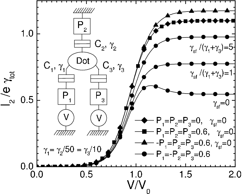
The system we have in mind is a quantum dot connected to three ferromagnetic leads $i\in\{1,2,3\}$, through tunnel junctions with capacitances $C_{i}$ and net spin-independent tunneling rates $\gamma_{i}$ (inset of Fig. 1). A voltage bias $V$ is applied to leads $1$ and $3$; lead $2$ is connected to ground. At voltages and temperatures much lower than the intrinsic level spacing and the charging energy $E_{C}=e^{2}/2C$ of the dot ($C=\sum_{i}C_{i}$), only one energy level of the dot located at $E_{0}$ needs to be taken into account. In this situation, the dot can either be empty, or occupied with one electron with spin $\sigma\in\{\uparrow,\downarrow\}$. Here and in the following, we will measure energies from the Fermi level, i.e., $E_{F}=0$.

The collinear magnetic polarizations $P_{j}$ of the leads are taken into account by using spin-dependent tunneling rates $\gamma_{j\sigma}=\gamma_{j}(1+\sigma P_{j})$, where $\sigma=\pm 1$ labels the electron spin. In a simple model, the spin-dependence is a consequence of the different densities of states for majority and minority electrons julliere:75. The rate for an electron to tunnel on/off the dot ($\epsilon=\pm 1$) through junction $j$ is then given by $\Gamma_{j\sigma}^{\epsilon}=\gamma_{j\sigma}/(1+\exp[\epsilon(E_{0}-eV_{j})/k_{B}T])$, where $V_{1}=V_{3}=-C_{2}V/C$, $V_{2}=(C_{1}+C_{3})V/C$. On the dot, there can be spin-flip scattering, for instance due to spin-orbit coupling or magnetic impurities. Here, we will assume that the on-site energy on the dot does not depend on spin. Hence, due to the detailed-balance rule, the spin-flip scattering rate $\gamma_{sf}$ does not depend on spin.

In the sequential-tunneling limit $\hbar\gamma_{j\sigma}\ll k_{B}T$, electronic transport through the dot can be described by the master equation setnoise; bulka:00:

where $p_{\psi}(t)$, $\psi\in\{\uparrow,\downarrow,0\}$, is the instantaneous occupation probability of state $\psi$ at time $t$, and where

depends on the total rates $\Gamma_{\sigma}^{\epsilon}=\sum_{j}\Gamma_{j\sigma}^{\epsilon}$ and $\gamma_{\sigma}=\sum_{j}\gamma_{j\sigma}$. The stationary occupation probabilities $\bar{p}_{\psi}$ are

and $\bar{p}_{0}=1-\bar{p}_{\uparrow}-\bar{p}_{\downarrow}$. They can be used to calculate the average value $\langle I_{j}\rangle$ of the tunneling current $I_{j}(t)$ through junction $j$ as $\langle I_{j}\rangle=e\sum_{\epsilon,\sigma}\epsilon\Gamma_{j\sigma}^{\epsilon}\bar{p}_{A(\sigma,-\epsilon)}$, where $A(\sigma,\epsilon)$ is the state of the dot after the tunneling of an electron with spin $\sigma$ in the direction $\epsilon$, i.e., $A(\sigma,-1)=0$, $A(\sigma,+1)=\sigma$.

In the following, we first consider the situation $E_{0}>0$. The voltage $V$ will always be assumed to be positive, such that it is energetically more favorable for electrons to go from the input electrode 2 to the output electrodes 1 or 3 than in the opposite direction. The typical voltage dependence of $I_{2}\equiv\langle I_{2}\rangle$ is shown in Fig. 1. The total current $I_{2}$ is exponentially suppressed at low voltages, increases around a voltage $V_{0}=E_{0}C/(C_{1}+C_{3})e$, and saturates at higher voltages. The width of the increase is determined by $k_{B}T/e$. The high-voltage limit of $I_{2}$ depends on the polarizations $P_{i}$ and rates $\gamma_{i}$ but not on the capacitances $C_{i}$. For a sample with magnetic contacts, this limit can be higher or lower than that of the paramagnetic case, depending on the parameters considered. In the high-voltage limit, $I_{2}(P_{1},P_{2},P_{3})-I_{2}(0,0,0)=2e\gamma_{c}P_{out}\langle S\rangle$, where $P_{out}=(P_{1}\gamma_{1}+P_{3}\gamma_{3})/(\gamma_{1}+\gamma_{3})$ is the net output lead polarization, $\langle S\rangle=\nu(P_{2}-P_{out})$ is the average spin accumulation on the dot Accumulation and $\gamma_{c}=\gamma_{2}(\gamma_{1}+\gamma_{3})/(\gamma_{1}+2\gamma_{2}+\gamma_{3})$. Here, $\nu$ is a positive function of the polarizations, the tunneling and scattering rates, which tends to $0$ at large $\gamma_{sf}$. Having a saturation current different from the paramagnetic case requires $P_{out}\neq 0$ and $\langle S\rangle\neq 0$. Spin-flip scattering modifies the $I_{2}-V$ curve once $\gamma_{sf}$ is of the order of the tunneling rates. It suppresses spin accumulation and makes the $I_{2}-V$ curve tend to the paramagnetic one.

The power spectrum of tunneling current correlations in leads $i$ and $j$ is defined as

where $\Delta I_{i}(t)=I_{i}(t)-\langle I_{i}\rangle$. The terms $\langle I_{i}(t)I_{j}(0)\rangle$ can be written as a function of the conditional probabilities $P_{\psi,\varphi}^{c}(t)$ which are the occupation probabilities of the state $\psi$ at time $t$ if at $t=0$ the state was $\varphi$, and which are zero for $t<0$. Solving Eq. (1) with the initial condition $P_{\psi,\varphi}^{c}(t=0)=\delta_{\psi,\varphi}$ leads to $P_{\psi,\varphi}^{c}(t)$. Its Fourier transform is given by $\hat{P^{c}}(\omega)=\int_{0}^{\infty}dt\exp(i\omega t)\hat{P^{c}}(t)=-(i\omega+\hat{M})^{-1}$. The eigenvalues of the matrix $\hat{M}$ thus govern the frequency dependence of $\hat{P}^{c}(\omega)$. The non-zero eigenvalues are $\lambda_{\pm}=\frac{1}{2}\left(-2\gamma_{sf}-\gamma_{\uparrow}-\gamma_{\downarrow}\pm\Delta\right)$, with $\Delta^{2}=4\gamma_{sf}^{2}+(\gamma_{\uparrow}-\gamma_{\downarrow})^{2}-4\gamma_{sf}(\Gamma_{\uparrow}^{+}+\Gamma_{\downarrow}^{+})+4\Gamma_{\uparrow}^{+}\Gamma_{\downarrow}^{+}$. This eventually leads to

where $S_{j}^{Sch}=2e^{2}\sum_{\epsilon,\sigma}\Gamma_{j\sigma}^{\epsilon}\bar{p}_{A(-\epsilon,\sigma)}$ is the Schottky noise produced by tunneling through junction $j$, and

Here, we defined $G_{\psi,\varphi}(\omega)=P_{\psi,\varphi}^{c}(\omega)+\bar{p}_{\psi}/i\omega.$

Equation (5) determines the full frequency-dependent tunneling current correlation functions of the three-terminal quantum dot. For frequencies larger than the cutoff frequencies $\lambda_{-}$ and $\lambda_{+}$, the spectrum $S_{ij}(\omega)$ tends to the uncorrelated spectrum $\delta_{ij}S_{j}^{Sch}$. In the following, we will consider mainly the zero-frequency limit of $S_{ij}(\omega)$, because the frequencies $\lambda_{\pm}\sim\gamma_{i}$ are difficult to access in experiment. Note that at zero frequency, the contribution of the screening currents ensuring electro-neutrality of the capacitors after a tunneling event buettiker:03-book is zero, i.e., $S_{ij}\equiv S_{ij}(0)$ is the signal measured in practice screening.

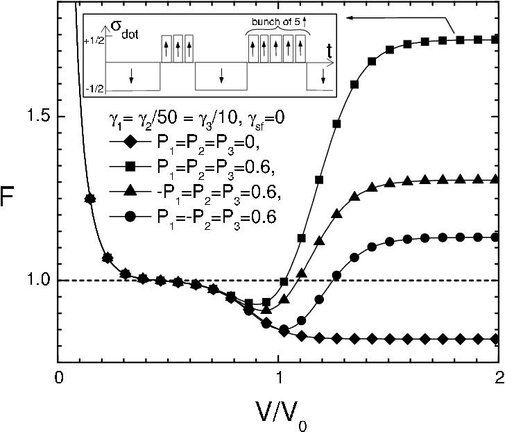
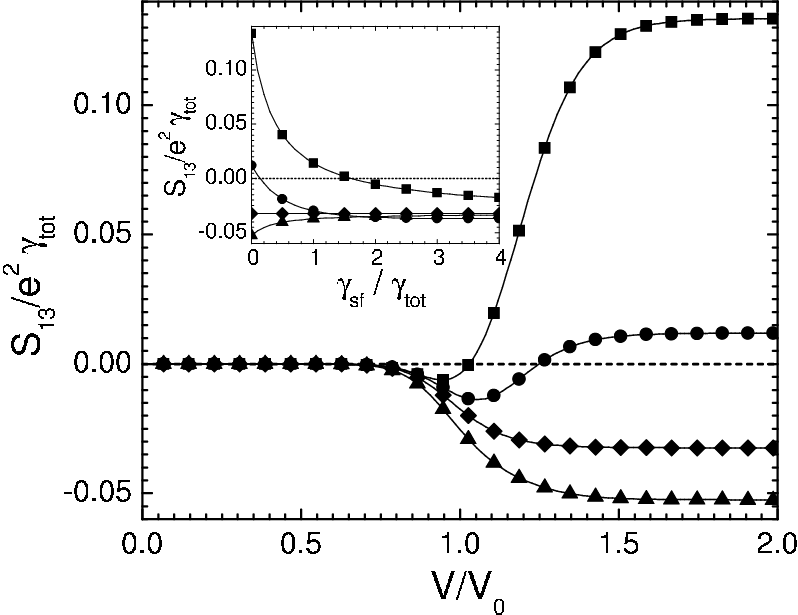
Figures 2, 3 show the Fano factor $F=S_{22}/2eI_{2}$ and the cross-correlations $S_{13}$ as a function of $V$ for $\gamma_{sf}=0$. Well below $V_{0}$ the current is due to thermally activated tunneling and the noise is Poissonian. At very low voltage, $eV\leq k_{B}T$, the cross-over to thermal noise is observed. Around $V=V_{0}$, $F$ and $S_{13}$ show a step or a dip. The high-voltage limit strongly depends on tunneling rates and polarizations. In the paramagnetic case, the limit of $F$ lies in the interval $[1/2,1]$, and that of $S_{13}/2eI_{2}$ in $[-1/8,0]$. In the ferromagnetic case the high-voltage limit of $F$ can be either sub- or super-Poissonian, as already pointed out in the two-terminal case bulka:99. Spin accumulation is not a necessary condition for having a super-Poissonian Fano factor, as can be seen for $P_{1}=P_{2}=P_{3}$, where $\left\langle S\right\rangle=0.$ In this case, the essential point is that the current can flow only in short time windows where the current transport is not blocked by a down spin, see the inset of Fig. 2. This dynamical spin blockade leads to a bunching of tunneling events, and explains the super-Poissonian Fano factor.

The cross-correlations can be either positive or negative, see Fig. 3. Note that a super-Poissonian $F$ does not necessarily imply positive cross-correlations, as shown by the case $-P_{1}=P_{2}=P_{3}=0.6$ in Figs. 2, 3, for which the cross-correlations are even more negative than in the paramagnetic case. Indeed, relations (5) and (6) together with charge conservation imply that $S_{22}-S_{2}^{Sch}=\sum_{\sigma,\sigma^{\prime}}S_{1,\sigma,3,\sigma^{\prime}}^{c}\left(\gamma_{1\sigma}+\gamma_{3\sigma}\right)\left(\gamma_{1\sigma^{\prime}}+\gamma_{3\sigma^{\prime}}\right)/\gamma_{1\sigma}\gamma_{3\sigma^{\prime}}$ at $V\gg V_{0}$. Thus, at $V\gg V_{0}$, a super-Poissonian $F$ is equivalent to positive cross-correlations only at large voltages and if the two output leads have identical polarisations. For the case $-P_{1}=P_{2}=P_{3}=0.6$, cross-correlations are negative in spite of the super-Poissonian $F$ because the correlated electrons are mostly up electrons flowing through lead 3. We note here that $\text{Re}[S_{13}(\omega)]$ can change sign for intermediate frequencies and vanishes for $\omega\gg\lambda_{+},\lambda_{-}$ unpublished.

We now briefly comment on the case $E_{0}<0$. For $V\gg V_{0}^{\prime}=-E_{0}C/C_{2}e$, the values of $I_{2}$, $F$ and $S_{13}$ are the same as previously. When $V$ is smaller than $V_{0}^{\prime}$, the most striking difference is that $F$ is polarization-dependent and thus not necessarily Poissonian.

The effect of spin-flip scattering is shown in the inset of Fig. 3. Spin-flip scattering influences the cross-correlations once $\gamma_{sf}$ is of the order of the tunneling rates. In the high-$\gamma_{sf}$ limit, cross-correlations tend to the paramagnetic case for any value of the polarizations. Thus, strong elastic spin-flip scattering suppresses positive cross-correlations, in contrast to what happens with inelastic scattering in texier:00. In practice, experiments with a quantum dot connected to ferromagnetic leads and $\gamma_{sf}\ll\gamma_{tot}$ have already been performed Deshmukh. Thus, spin-flip scattering should not prevent the observation of positive cross-correlations in quantum dots.

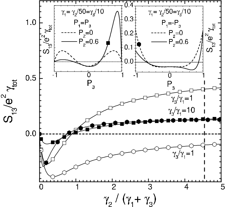
Finally, we address the problem of how to choose parameters that favor the observation of positive cross-correlations. First, finite lead polarizations are necessary bagrets:02, see the insets of Fig. 4. However, it is possible to get positive cross-correlations even if $P_{2}=0$, provided the output leads 1,3 of the device are sufficiently polarized (dashed lines in the insets of Fig. 4). The case where the three electrodes are polarized in the same direction seems the most favorable. In the high-voltage limit, choosing $P_{1}=P_{2}=P_{3}$ and $\gamma_{sf}=0$ leads to

The asymmetry between the tunneling rates $\gamma_{i}$ has a strong influence on the cross-correlations, see Fig. 4. Large values of $\gamma_{2}/(\gamma_{1}+\gamma_{3})$ favor the observation of positive cross-correlations, see e. g. Eq. (7), by decreasing $\bar{p}_{0}$. This allows to extend the domains of positive cross-correlations to smaller values of the polarizations, which is important because experimental contact materials are not fully polarized. For $\gamma_{1}=\gamma_{2}/10=\gamma_{3}$, the polarizations $P_{1}=P_{2}=P_{3}=0.4$ typical for Co Soulen lead to positive cross-correlations of the order of $S_{13}/e^{2}\gamma_{tot}\simeq 0.08$. With $\gamma_{tot}\simeq 5$GHz this corresponds to $10^{-29}$A²s, a noise level accessible with present noise-amplification techniques birk:95.

In conclusion, we have demonstrated that transport through a multi-terminal quantum dot with ferromagnetic contacts is characterized by a new mechanism, viz., dynamical spin blockade. As one of its consequences we predict positive current cross-correlations in the drain contacts without requiring the injection of correlated electron pairs. We have included spin-flip scattering on the dot and have shown that the effect persists as long as the spin-flip scattering rate is less than the tunneling rate to the contacts.

We thank T. Kontos and C. Schönenberger for useful discussions. This work was financially supported by the RTN Spintronics, by the Swiss NSF, and the NCCR Nanoscience.

References

- (1) Ya. M. Blanter and M. Büttiker, Phys. Rep. 336, 1 (2000).
- (2) Quantum Noise in Mesoscopic Physics, edited by Yu. V. Nazarov (Kluwer, Dordrecht, 2003).
- (3) V. A. Khlus, Sov. Phys. JETP 66, 1243 (1987).
- (4) G. B. Lesovik, JETP Lett. 49, 592 (1989).
- (5) M. Büttiker, Phys. Rev. Lett. 65, 2901 (1990).
- (6) M. Büttiker, Phys. Rev. B 46, 12485 (1992).
- (7) M. Henny et al., Science 284, 296 (1999); W. D. Oliver et al., Science 284, 299 (1999); S. Oberholzer et al., Physica (Amsterdam) E 6, 314 (2000).
- (8) See the article of M. Büttiker, in Ref. nazarov:03.
- (9) T. Martin, Phys. Lett. A 220, 137 (1996); M. P. Anantram and S. Datta, Phys. Rev. B 53, 16390 (1996); J. Torres and T. Martin, Eur. Phys. J. B 12, 319 (1999); T. Gramespacher and M. Büttiker, Phys. Rev. B 61, 8125 (2000); J. Torres et al., ibid. 63, 134517 (2001); J. Börlin et al., Phys. Rev. Lett. 88, 197001 (2002); P. Samuelsson and M. Büttiker, ibid. 89, 046601 (2002); Phys. Rev. B 66, 201306 (2002); F. Taddei and R. Fazio, ibid. 65, 134522 (2002).
- (10) A. M. Martin and M. Büttiker, Phys. Rev. Lett. 84, 3386 (2000).
- (11) A. Cottet et al., to be published elsewhere.
- (12) C. Texier and M. Büttiker, Phys. Rev. B 62, 7454 (2000).
- (13) I. Safi et al., Phys. Rev. Lett. 86, 4628 (2001); A. Crepieux et al., Phys. Rev. B 67, 205408 (2003).
- (14) A. N. Korotkov, Phys. Rev. B 49, 10381 (1994); S. Hershfield et al., ibid. 47, 1967 (1993); U. Hanke et al., ibid. 48, 17209 (1993).
- (15) D. Loss and E. V. Sukhorukhov, Phys. Rev. Lett. 84, 1035 (2000); E. V. Sukhorukov et al., Phys. Rev. B 63, 125315 (2001); D.V. Averin, in Macroscopic Quantum Coherence and Quantum Computing, edited by D.V. Averin, B. Ruggiero, and P. Silvestrini (Kluwer, Dordrecht, 2001); cond-mat/0010052.
- (16) H. Birk et al., Phys. Rev. Lett. 75, 1610 (1995).
- (17) D. A. Bagrets and Yu. V. Nazarov, Phys. Rev. B 67, 085316 (2003).
- (18) B. R. Bulka et al., Phys. Rev. B 60, 12246 (1999).
- (19) B. R. Bulka, Phys. Rev. B 62, 1186 (2000).
- (20) M. Julliere, Phys. Lett. A 54, 225 (1975).
- (21) J. Barnas and A. Fert, Phys. Rev. Lett. 80, 1058 (1998); S. Takahashi and S. Maekawa, ibid. 80, 1758 (1998); J. Barnaś and A. Fert, Europhys. Lett. 44, 85 (1998); F. Guinea, Phys. Rev. B 58, 9212 (1998); H. Imamura et al., ibid. 59, 6017 (1999); A. Brataas et al., Eur. Phys. J. B 9, 421 (1999); X.H. Wang and A. Brataas, Phys. Rev. Lett. 83, 5138 (1999).
- (22) The total current correlations, including screening currents, are
- (23) M. Deshmukh and D. C. Ralph, Phys. Rev. Lett. 89, 266803 (2002).
- (24) M. Soulen et al., Science 282, 85 (1998).