Competing orders in thermally fluctuating superconductors
in two dimensionsPreprint: cond-mat/0308024
Abstract
We extend recent low temperature analyses of competing orders in the cuprate superconductors to the pseudogap regime where all orders are fluctuating. A universal continuum limit of a classical Ginzburg-Landau functional is used to characterize fluctuations of the superconducting order: this describes the crossover from Gaussian fluctuations at high temperatures to the vortex-binding physics near the onset of global phase coherence. These fluctuations induce affiliated corrections in the correlations of other orders, and in particular, in the different realizations of charge order. Implications for scanning tunnelling spectroscopy and neutron scattering experiments are noted: there may be a regime of temperatures near the onset of superconductivity where the charge order is enhanced with increasing temperatures.
I Introduction
A number of recent perspectives zaanennat; pnas; science; so5; sachdev_zhang; srmp; krmp have highlighted new experimental lake; halperin; boris; lake2; seamus; howald and theoretical kwon; prl; vadim; tolyastm; vojta; zaanen; podolsky; chenting; zhu; franz; zhang; ghosal; andersen02 works exploring the interplay between the multiple order parameters which characterize the ground state of some of the cuprate superconductors. Good evidence was obtained for a strong coupling between the superconducting order and density wave order in spin/charge/bond correlations (described more precisely below). In particular, by tuning the superconducting order by an applied magnetic field at very low temperatures (), a strong field-dependent variation was observed in the latter correlations.
In this paper, we explore the possibility of observing related connections in the finite temperature ‘pseudogap’ region above the superconducting critical temperature, . Here, the superconducting order has strong dependent fluctuations; we will compute these fluctuations in the framework of a two-dimensional Ginzburg-Landau theory, including a precise characterization of strong fluctuations obtained from numerical studies. We will show that the model of Ref. prl predicts that such fluctuations lead to a corresponding sympathetic variation in the autocorrelations of the other orders. Working to linear order in the coupling between superconductivity and these orders, we provide a computation of certain universal characteristics of the dependence of the latter fluctuations. Our results will also be formally extended to for completeness, but it must be noted that we neglect the inter-layer coupling and quantum effects, which become important at lower 3d.
We begin by defining the order parameters under consideration. The primary order is the complex superconducting order which describes the spatial variation in the order associated with condensation of Cooper pairs. This is expected to undergo strong ‘phase’ fluctuations phase for near . Using the proximity of the underdoped cuprates to a superfluid-insulator quantum transition, Refs. ssrelax; nature argued that ‘amplitude’ fluctuations should be treated at an equal footing gap, and proposed that such thermal fluctuations could be described by a classical partition function of a suitable universal continuum limit of the Ginzburg-Landau free energy: this will be reviewed here in Section III. Such an approach describes the crossover from Gaussian superconducting fluctuations at temperatures well above , to the vortex physics of the Kosterlitz-Thouless transition near . A dynamic theory with a similar static component (although with a lattice cutoff) was recently used huse1; ussi; huse2 to describe the notable measurements ong of the Nernst effect.
This fluctuating superconductor is also expected to have appreciable correlations in other order parameters. The spin-density-wave order is described by the complex 3-component vectors , , where extends over the 3 spin directions, and the spin operator on site , is given by
| (1) |
Here are the spin-density-wave ordering wavevectors along the and principle axes of the square lattice: near a doping of , we have and . In a similar manner we can define bond order parameters by examining the modulations in the exchange energy of a pair of spins separated by a distance :
| (2) |
The special case of is a measure of the charge density wave order. Comparison between (2) and (1) suggests that the ordering wavevectors are related by , and this is observed experimentally.
A number of other order parameters which are invariant under spin rotations, like , can also be defined prl; podolsky. These include the site charge density, the average electron kinetic energy in a bond, or modulations in the pairing amplitude. By symmetry, all such quantities will have modulations at the wavevectors , and we can therefore expect that their order parameter fluctuations will track those of . Differences in microscopic physics can, of course, make some of these modulations much larger than others. We will not explicitly consider all such possibilities here, and the reader should view as a suitable representative of the order parameters characterizing modulations at the wavevectors in observables invariant under spin rotations. We will subsequently refer to the order represented by simply as charge order.
While the focus of this paper is on the interplay between the superconducting fluctuations and the orders mentioned above, it should be clear to the reader that our considerations are quite general. Simple extensions lead to similar effects in the interplay of superconductivity with most of the other orders in the zoo of possibilities considered in the theory of the cuprates.
In considering correlations of , and in the fluctuation region, it is important to consider the influence of random static impurities which are invariably present in the cuprates. As almost all impurities preserve electron number and spin rotation invariance, their influence on and will consist of perturbations in the random exchange class (this is discussed more explicitly in Section II). In contrast, the order breaks only lattice symmetries, and is consequently subject to the far more disruptive random field perturbations apy. In two spatial dimensions, this implies that true long-range order cannot develop as , and that the correlation length saturates at a finite value. We will assume here that there is a local onset of , , and orders at temperatures where the pseudogap develops, but at lower temperatures correlations are predominantly controlled by the random-field disorder, and have only a weak, intrinsic dependence. This is also consonant with the result that thermal fluctuations are irrelevant at the random-field transition in higher dimensions apy. In contrast, the fluctuations of and are strongly dependent, and can have an infinite correlation length as . The order becomes quasi-long-ranged at and has the strongly -dependent Gaussian-to-vortex crossover noted above at . The order can also have the exponential rapid dependence associated with the breaking of O(3) spin rotation symmetry as .
This paper will consider the regime above where
| (3) |
The non-zero value is due to the presence of random-field perturbations which explicitly break lattice symmetries, and so allow to locally have a non-zero mean value which will fluctuate randomly as a function of . As noted above, we assume that only has a weak intrinsic dependence. However, the fluctuations of the , , and orders are not independent, and so the strong dependence associated with the Gaussian-to-vortex crossover in will induce a corresponding -dependent variation in . This paper will compute this variation and suggest associated experimental tests. Strictly speaking, because there is only quasi-long-range order in below , the expectation values (3) apply also for : indeed, our methods and results extend also to . However, as noted earlier, we neglect the effects of inter-layer couplings and of quantum fluctuations, and so our low results should be treated with caution.
Our theory for the fluctuating orders and their interplay is summarized in Section II, which also contains are main results. Details of the continuum theory of the superconducting fluctuations and its Gaussian-to-vortex crossover appear in Section III. Section IV discusses experimental tests and possible extensions of our theory.
II Correlations between fluctuating orders: main results
This section will introduce the free energies which control the fluctuations of the order parameters, and state our main results on the dependence of the order at .
We describe the fluctuations of the superconducting order by a classical continuum partition function over the Ginzburg-Landau free energy ssrelax
| (4) |
We use here the notation of Refs huse1; ussi; huse2: , , are parameters which can be computed, in principle, from the microscopic physics of the underlying electrons. The co-efficient of , , vanishes at a mean-field transition temperature, , which will be distinct from the temperature at which there is a Kosterlitz-Thouless transition i.e. . The purely two-dimensional, and classical theory (4) is expected to apply to the cuprates only for : below we have to also account for three-dimensional effects arising from inter-layer couplings, and for quantum effects at low enough . All such effects will be neglected here, but for completeness, we will nevertheless discuss properties of the theory (4) over the full range of values.
An important point is that the functional integral in (4) is not defined on its own, and needs an ultraviolet regulator. In the physical system this is provided by the underlying electron physics on the lattice, but this is very difficult to characterize explicitly. Here, we shall follow the procedure proposed in Ref. ssrelax: the ultraviolet dependence can be accounted for by a suitable renormalization in the value of . However, because we do not know the explicit form of the ultraviolet cutoff, we cannot a priori compute the needed shift in . This lack of knowledge can be circumvented by using the experimental value of as an input into our calculation. The knowledge of the actual , combined with the parameters in (4) then allows a quantitative computation of the Gaussian-to-vortex crossover with no free parameters. We re-iterate that (4) cannot be regarded as a fully predictive theory on its own, and so cannot, even in principle, predict the actual value of : once is determined by other means, precise quantitative predictions for other observables become possible.
The Gaussian-to-vortex crossover can be expressed in terms of the following dimensionless parameter
| (5) |
The parameter should be a monotonically increasing function of . For , , at , we have , and above , takes positive values. We will see later that the present continuum theory eventually breaks down at large , when begins to acquire a non-monotonic dependence on . The value of is a measure of the strength of corrections to the mean field theory of .
It is important to note that the dependence of in (4) and (5) is non-universal, and this will lead to some non-universality in the dependence of all our predictions. However, one of our main points is that there is a universal dependence on the parameter . Moreover, once we assume a linear dependence of near (as is commonly done, and we will do in (22)), the dependence of our predictions becomes specific.
Aided by the results of Ref. ssrelax; nikolay1; nikolay2 we will show that it is possible to obtain precise predictions for a variety of correlators of . We quote a result which will be useful in our analysis here of multiple order parameters:
| (6) |
where is a universal function. The averages on the left-hand-side are evaluated under the partition function at the indicated temperature. We will show in Section III that it is possible to re-express the two argument function in terms of a single argument function as in (21), where depends upon and as in (20). Here we present results for the initial crossover from the Gaussian to the vortex regime, which occurs when :
| (7) | |||||
The numerical constants appearing in the arguments of the logarithms are universal. These constants, and the constants appearing in the arguments of all subsequent logarithms, depend on only two universal numbers that have to be determined by computer simulations: the latter numbers are the constant computed first in Ref. ssrelax, and the constant computed in Refs. nikolay1; nikolay2. Additional higher order terms in (7) have also been computed and these will be presented in Section III: we show there that it is possible to account for all logarithmic terms that appear at higher orders in . Numerical results for the full range of values of appear in Section III. The expression (6) has ignored the possible -dependencies of and for simplicity: it is possible to account for these in a similar manner, as will become clear from the discussion in Section III.
It is worth noting here that vortices are already present in the Gaussian theory, associated with zeros of bert. The result (7) accounts for the initial correlations between these vortices, but does not include the vortex-binding physics of the Kosterlitz-Thouless transition. The latter is only accounted for by the numerical results in Section III.
Let us turn now to the density wave order parameters , . The complete effective action for these order parameters has a rather complicated structure and was discussed in Ref. prl. A simple Gaussian form will be satisfactory for our purposes here:
| (8) | |||||
Apart from the usual Gaussian terms prl, the above contains
complex random fields and which pin the ‘sliding’ mode of the charge density wave.
These fields arise from impurities which preserve spin rotation
invariance: as a consequence, notice that the random coupling is
linear in the fields , but that there is only a
random-exchange coupling to O(3) rotations in the spin density
wave order. These simple facts have a number of interesting
implications:
(i) There can be no long range charge order in two spatial
dimensions, even at . This implies that there can be no
quantum critical point, tuned by the hole concentration,
associated with the onset of such order. A quantum critical point
associated with the restoration of O(3) symmetry
remains possible.
(ii) The strong relevance of such random-field
perturbations suggests that in the absence of couplings to other
critical order parameters, the correlation length
can be assumed to be roughly temperature-independent at low temperatures.
(iii) The theories (4) and (8) describe a
phase in which the expectation values in (3) hold.
Finally, as promised, let us consider the influence of the fluctuations described by on the charge order correlations. The simplest coupling between the orders is a term, and, as in Ref. prl, this leads to the leading order correction
| (9) |
Here is the ‘bare’ correlation length of the order, which is expected to be only temperature dependent near . We input the value of as computed in (6) and Section III, and obtain our main predictions for the superconducting fluctuation-induced modification in the correlation length.
III Continuum theory of thermal superconducting fluctuations
This section will review the results of Ref ssrelax relevant to obtaining (6) and (7) and its extensions. Appendix A will review the work of Prokof’ev, Ruebenacker, and Svistinov nikolay1; nikolay2 on the dilute two-dimensional Bose gas and show that the results of their numerical simulations can be mapped onto universal quantities needed here.
Ref. ssrelax studied the following continuum theory of a component real scalar , :
| (10) |
(Here we have changed notation for the field, from in Ref. ssrelax, to here, to prevent confusion with the spin density wave order.) This theory maps onto (4) with the following correspondences:
| (11) |
It was argued ssrelax that the continuum limit of required only the single renormalization of to :
| (12) |
Here we have introduced an ultraviolet cutoff which is needed to regulate the theory . The renormalization in (12) is associated with logarithmic ultraviolet divergence of the one-loop ‘tadpole’ diagram; the renormalized in the propagator on the right-hand-side accounts for tadpoles-on-tadpoles etc. All other diagrams are ultraviolet convergent, and hence the simple structure of the renormalization theory.
It is important to note that (12) is the exact definition of , and consequently is not the fully ‘self-energy’ of the field at zero external momentum; only accounts for the resummation of tadpole graphs. In practice, the relationship (12) implies that, when we perform a Feynman graph expansion of any observable, we can ignore all tadpole graphs, and replace by in all propagators. Notice also that as the bare coupling extends from to , the renormalized coupling extends from 0 to .
After the renormalization of to , all subsequent correlators of are ultra-violet convergent, and so we can safely take in them. This implies that all these correlators are universal functions of the single dimensionless quantity that can be obtained from the parameters in (10): this is the analog of the ‘Ginzburg ratio’, defined here as
| (13) |
For , where , we have . Conversely, for , and .
The field theory (10) exhibits a Kosterlitz-Thouless transition at some critical temperature, and the arguments above imply that this transition occurs at a universal critical value . The numerical studies of Ref. ssrelax found . The value of can also be obtained from the subsequent, and more precise, numerical simulations of Refs. nikolay1; nikolay2; this connection is discussed in Appendix A, and (29) yields
| (14) |
We are interested here in the value of . This quantity requires a single additive renormalization before the continuum limit is obtained; hence we can write
| (15) |
where is a universal function. A number of analytic results for this universal function can be obtained from the methods of Ref ssrelax, and details appear in Appendix B. For (corresponding to ), perturbation theory in powers of about the saddle point yields
| (16) |
All subsequent terms in the above expansion involve only integer powers of and there are no logarithms. For (corresponding to ), we expand about a saddle point with . As shown in Ref. ssrelax, this is done by introducing a ‘dual’ coupling related to by
| (17) |
Note that as , . For large , the expansion of is
| (18) |
All subsequent terms in the present expansion involve only integer powers of , with no additional logarithms. As discussed in Appendix A, the numerical results of Ref. nikolay1; nikolay2 yield the values of for all values of . In particular, at the critical point we have from (32)
| (19) |
The theory of the Kosterlitz-Thouless transition implies that will have a weak essential singularity at , similar to that in the specific heat. A plot of the values of appears in Fig 1. It is interesting to note that either the small or the small expansions is accurate for the entire range of values.
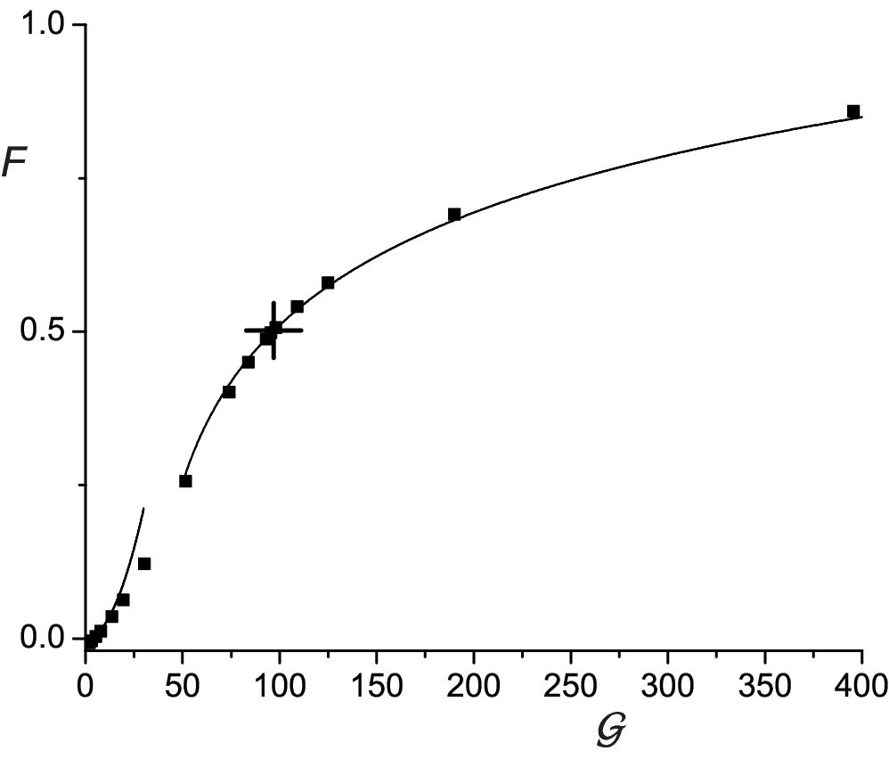
The discussion so far presents our most complete results for the properties of and with essentially no approximations. There is, however, still some residual cutoff dependence. This can be removed by subtracting corresponding results at two different values of the bare coupling (or ), while fixed. Depending upon the physical situation, changing may also involve some changes in the values of . However, such changes are expected to be small and we neglect any dependence in and in the remainder of this section. This allows to obtain an explicit relation between the dimensionless number used in the present section, and the number in (5). Dividing (12) by and subtracting the corresponding equation at the critical point, and using the definitions in (11) and (13), we obtain
| (20) |
As expected, extends from to as extends from 0 to . Applying the same procedure to (15) we obtain the universal function in (6)
| (21) |
The expressions (14), (16)-(21) constitute the central results of this paper. Using as input the values of and , we compute from (20) and from (17); then using results (16) and (18) we can compute ), and finally insert in (21) to obtain . In particular, the small expansion in (16) yields (7). Of course, it is better to numerically solve for from (20), rather than obtaining the solution order-by-order in as was done for (7).
We now present some numerical results for the parameters used by Mukerjee and Huse huse2. They set . Inserting this in (5) yields
| (22) |
The parameterization is chosen to be valid near , but can also be reasonably extended as (in BCS theory, we expect a divergent , but this divergence is expected to be cutoff near a superfluid-insulator transition). By in (22), we mean the value of the helicity modulus of extrapolated to in this manner (the London penetration depth is related to the helicity modulus by ). It is worth noting here that and are, in general, independent of each other, and the Nelson-Kosterlitz relation nk only constrains .
This framework now predicts all physical properties with 2 input parameters: the values of and . Mukerjee and Huse huse2 also defined a parameter as a measure of the strength of fluctuations. This is related to the parameters used here by . In our numerical results below, we set , following their parameters.
An important subtlety should be noted here. The use of (22) in (20) normally yields a value for which decreases monotonically with increasing , as seems reasonable, given our understanding of physical properties of the continuum theory. However, because the value of in (22) saturates as and because of the presence of the term on the right-hand-side of (20), for very the value of eventually starts increasing with increasing . This is clearly unphysical, and is an indication that the present continuum theory breaks down at large enough . For the value of being used here, this unphysical non-monotonicity arises only at , and we will therefore restrict our attention to values of below this.
Solving (22) and (20) for as a function of , we use the results of this section and Appendix A to obtain the plot of Fig 2 for the quantity appearing in (9).

Note, again that either the small or the large expansion is reasonable accurate.
IV Conclusions
We conclude this paper by discussing some of the experimental and broader implications of our work.
Our primary result (9) for the coherence length of the charge order can be tested against neutron scattering and scanning tunnelling spectroscopy (STS) experiments. However, the strong random field disorder may make inaccessible to a neutron probe which averages over the entire sample. In contrast, STS provides a local probe, and so may be more sensitive to the effects discussed here.
Consider an STS experiment with a field of view of area , such as those performed in Refs. seamus; howald; krmp; seamus2; ali. Quasiparticle interference contributions, such as those computed in Ref. dunghai; doug; tolyastm; franz2; yeh, appear at low temperatures, but we can expect that these will significantly broaden at temperartures above . We therefore focus here only on the contribution of the fluctuations, which also lead to modulations in the local density of the states measured in STS, as shown in Ref. tolyastm; yeh. We know that the STS measurements are in the linear response regime. So, when we perform the Fourier transform of the local density of states at the ordering wavevector , we find that the signal is proportional to the uniform part of the charge order parameter, . Let us estimate . We have for the free energy
| (23) |
Here we used that the result that the random field energy scales as the square root of the area. We can now minimize (23) with respect to
| (24) |
Taking from Eq. (9) obtain get the temperature dependence of the STS signal at the wavevector .
For the case of competition between the superconducting () and charge () orders, the coupling in (9) will be positive. In this situation we have a seemingly counterintuitive effect: as is increased through , the amplitude of the charge order is enhanced. The physical origin of this is not difficult to understand: the increase in phase coherence as is lowered is associated with an enhanced coherent motion of the Cooper pairs, and this leads to a decrease in the amplitude of the spatial modulations foot.
An alternative statement of the same physics can be made in terms of the vortices. As we argued in Ref. prl, vortices nucleate static charge order, and this was proposed as an explanation of the experiments of Ref. seamus (other approachesso5; chenting; zhu; zhang; ghosal; andersen02 have proposed static spin order in the vortices—in our theory, static spin order is not nucleated by vortices and appears only in phases with global magnetic order prl). Increasing above causes a proliferation of vortices, and hence an enhancement of charge order.
While our discussion in this paper has been entirely at the level of the Landau theory of multiple order parameters, it is important to keep in mind that such a theory is an effective model, and does not preclude other interpretations which focus directly on the electronic quasiparticles. In particular we can view the competition between charge order and superconductivity as the competition for the ordering of low energy quasiparticles near the Fermi surface. So as the superconducting pairing of these quasiparticles is reduced above , they are more susceptible to charge ordering.
An interesting direction for future work is to combine the continuum theory of the Ginzburg-Landau functional presented here with the theory of time-dependent superconducting fluctuations presented in Refs. huse1; ussi; huse2: this has the prospect of placing more precise quantitative constraints on the analysis of the Nernst effect experiments. Moreover, the accuracy of either the small or large expansions suggests that useful analytic results may be possible. Results for the fluctuation conductivity in such an approach, including corrections to the Aslamazov-Larkin fluctuation conductivity, have appeared recently sscond. A similar dynamic approach can also be applied to computing the linewidths of the electronic quasiparticles in the pseudogap regime: the strong amplitude fluctuations in should lead to significant broadening in the electronic spectral functions measured in photoemission experiments.
Acknowledgements.
We thank A. Yazdani for numerous stimulating discussions in which he proposed a related physical picture. We also thank J. C. Davis, J. Hoffman, A. Kapitulnik, S. Kivelson, D. H. Lee, D. Podolsky, N. Prokof’ev, B. Svistinov, N.-C. Yeh, A. P. Young, and S.-C. Zhang for useful discussions. This research was supported by US NSF Grants DMR-0098226 (S.S.) and DMR-0132874 (E.D.) and the Sloan Foundation.Appendix A Correspondence with the dilute Bose gas
This appendix discusses the connection between the analysis of the dilute Bose gas in Refs. nikolay1; nikolay2 and the results of Ref. ssrelax and the present paper. Let us make it clear at the outset that we are not advocating a dilute Bose gas description of the underdoped cuprates; rather, the finite temperature properties of the dilute Bose gas are characterized by some universal numbers which appear also in the models of interest in the present paper.
The dilute Bose gas is defined by the partition function
| (25) |
We follow the notation of Refs. nikolay1; nikolay2 throughout this appendix. The only exception is that the boson interaction has been replaced by , to prevent confusion with the coupling in (10).
Integrating out the non-zero Matsubara frequency modes in the Bose gas, the action for the zero frequency modes takes the form (10) with the coupling constants
| (26) |
The integral above is divergent in the ultraviolet, but if we use (12) to obtain the value of the renormalized coupling we obtain a convergent integral:
| (27) | |||||
In the last expression we have expanded to leading order in , as required from consistency with previous approximations. Now using the definition of the dimensionless coupling in (13), we obtain the value of the chemical potential at the Kosterlitz Thouless transition
| (28) |
with universal number computed in Ref. nikolay1 related to the universal number computed earlier in Ref. ssrelax by
| (29) |
Refs. nikolay1; nikolay2 obtained , which is in reasonable agreement with the value obtained in Ref. ssrelax; the latter value of yields from (29).
The same method can be used to compute the boson density . Integrating out the non-zero frequency modes and mapping onto the classical theory (10) we obtain
| (30) | |||||
in the last equation we have made the same simplification as that in the last equation in (27). The result (30) yields the expression obtained in Ref. nikolay1 for the critical density
| (31) |
with the universal number given by
| (32) |
The simulations of Refs. nikolay1; nikolay2 obtained , and inserting this result in (32) allows us to compute .
Appendix B Weak and strong coupling expansions
This appendix presents discusses the expansion for the universal function appearing in (15) for small and large
For small , a simple Feynman graph expansion of (10) can be carried out to order , with the diagrams shown in Fig 3.

All propagators in Fig 3 involve the bare ‘mass’ . A simple calculation shows that the graphs (a,b,c,e) are all absorbed by the first term on the right-hand-side of (15), after substitution of (12). This is a simple example of our claim that all ‘tadpole’ diagrams can be neglected after substituting for . Only Fig 3d contributes to in (15), and yields
| (35) | |||||
We evaluated the last integral numerically and obtained (16).
For large , the method described in Appendix C of Ref. ssrelax was used. To one loop order, the result
| (36) |
is easily obtained, where, as in Ref. ssrelax, . In obtaining (36), we have to explicitly account for all tadpole graphs, and the relationship in (2.4) of Ref. ssrelax between and . The large momentum behavior of the expansion about and saddle points should be the same, and this ensures that the ultraviolet divergences cancel. At two loop order, 35 Feynman graphs appear; these were evaluated as in Appendix C of Ref. ssrelax, and their sum was found to vanish. Consequently, there is no order term in , and the result (18) follows.
References
- (1) J. Zaanen, Nature 404, 714 (2000).
- (2) V. J. Emery, S. A. Kivelson, and J. M. Tranquada, Proc. Natl. Acad. Sci. USA 96, 8814 (1999).
- (3) S. Sachdev, Science 288, 475 (2000).
- (4) S.-C. Zhang, Science 275, 1089 (1997).
- (5) S. Sachdev and S.-C. Zhang, Science 295, 452 (2002).
- (6) S. Sachdev, Rev. Mod. Phys. 75, 913 (2003).
- (7) S. A. Kivelson, E. Fradkin, V. Oganesyan, I. P. Bindloss, J. M. Tranquada, A. Kapitulnik, and C. Howald, Rev. Mod. Phys. 75, 1201 (2003).
- (8) S. Katano, M. Sato, K. Yamada, T. Suzuki, and T. Fukase, Phys. Rev. B 62, R14677 (2000).
- (9) B. Lake, G. Aeppli, K. N. Clausen, D. F. McMorrow, K. Lefmann, N. E. Hussey, N. Mangkorntong, M. Nohara, H. Takagi, T. E. Mason, and A. Schröder, Science 291, 1759 (2001).
- (10) V. F. Mitrović, E. E. Sigmund, M. Eschrig, H. N. Bachman, W. P. Halperin, A. P. Reyes, P. Kuhns, and W. G. Moulton, Nature 413, 501 (2001).
- (11) B. Khaykovich, Y. S. Lee, R. W. Erwin, S.-H. Lee, S. Wakimoto, K. J. Thomas, M. A. Kastner, and R. J. Birgeneau, Phys. Rev. B 66, 014528 (2002).
- (12) B. Lake, H. M. Rønnow, N. B. Christensen, G. Aeppli, K. Lefmann, D. F. McMorrow, P. Vorderwisch, P. Smeibidl, N. Mangkorntong, T. Sasagawa, M. Nohara, H. Takagi, T. E. Mason, Nature 415, 299 (2002).
- (13) J. E. Hoffman, E. W. Hudson, K. M. Lang, V. Madhavan, S. H. Pan, H. Eisaki, S. Uchida, and J. C. Davis, Science 295, 466 (2002).
- (14) C. Howald, H. Eisaki, N. Kaneko, and A. Kapitulnik, cond-mat/0201546; C. Howald, H. Eisaki, N. Kaneko, M. Greven, and A. Kapitulnik, Phys. Rev. B, 67, 014533, (2003).
- (15) K. Park and S. Sachdev, Phys. Rev. B 64, 184510 (2001).
- (16) E. Demler, S. Sachdev, and Y. Zhang, Phys. Rev. Lett. 87, 067202 (2001); Y. Zhang, E. Demler, and S. Sachdev, Phys. Rev. B66, 094501 (2002).
- (17) S. A. Kivelson, D.-H. Lee, E. Fradkin, and V. Oganesyan, Phys. Rev. B 66, 144516 (2002).
- (18) A. Polkovnikov, M. Vojta, and S. Sachdev, Phys. Rev. B 65, 220509 (2002); A. Polkovnikov, S. Sachdev, and M. Vojta, Physica C 388-389, 19 (2003).
- (19) M. Vojta, Phys. Rev. B 66, 104505 (2002).
- (20) J. Zaanen and Z. Nussinov, Physica Status Solidi B, 236, 332 (2003).
- (21) D. Podolsky, E. Demler, K. Damle, and B. I. Halperin, Phys. Rev. B, 67, 094514 (2003).
- (22) Y. Chen and C. S. Ting, Phys. Rev. B 65, 180513 (2002).
- (23) J.-X. Zhu, I. Martin, and A. R. Bishop, Phys. Rev. Lett. 89, 067003 (2002).
- (24) M. Franz, D. E. Sheehy, and Z. Tesanovic, Phys. Rev. Lett. 88, 257005 (2002).
- (25) H.-D. Chen, J.-P. Hu, S. Capponi, E. Arrigoni, and S.-C. Zhang, Phys. Rev. Lett. 89, 137004 (2002).
- (26) A. Ghosal, C. Kallin, and A. J. Berlinsky, Phys. Rev. B 66, 214502 (2002).
- (27) B. M. Andersen, P. Hedegard, and H. Bruus, Phys. Rev. B 67, 134528 (2003).
- (28) Three-dimensional effects are also important in a narrow window of temperatures above , where the transition crosses over to the XY universality class. Such effects will be neglected here.
- (29) V. J. Emery and S. A. Kivelson, Nature 374, 434 (1995); N. Trivedi and M. Randeria, Phys. Rev. Lett. 75, 312 (1995); M. Franz and A. J. Millis, Phys. Rev. B 58, 14572 (1998); H.-J. Kwon and A. T. Dorsey, Phys. Rev. B 59, 6438 (1999).
- (30) S. Sachdev, Phys. Rev. B 59, 14054 (1999).
- (31) S. Sachdev and O. Starykh, Nature 405, 322 (2000).
- (32) It is important to distinguish ‘amplitude fluctuations’ in the superconducting order from the ‘pairing gap’ of the electrons. The former measures the strength of the superconducting correlations, while the latter is an energy gap associated with the fermionic spectrum at high energies. In particular, at low near a superconductor-insulator transition it was argued in Refs ssrelax; nature that the amplitude fluctuations become very strong. In contrast, the gap in the electron spectrum remains finite across such a transition.
- (33) I. Ussishkin, S. L. Sondhi, and D. A. Huse, Phys. Rev. Lett. 89, 287001 (2002).
- (34) I. Ussishkin, Phys. Rev. B 68, 024517 (2003).
- (35) S. Mukerjee and D. A. Huse, cond-mat/0307005.
- (36) T. T. M. Palstra, B. Batlogg, L. F. Schneemeyer and J. V. Waszczak, Phys. Rev. Lett. 64, 3090 (1990); H. C. Ri, R. Gross, F. Gollnik, A. Beck, R. P. Huebener, P. Wagner, and H. Adrian, Phys. Rev. B. 50, 3312 (1994); Z. A. Xu, N. P. Ong, Y. Wang, T. Kakeshita, and S. Uchida, Nature 406, 486 (2000); Y. Wang, Z. A. Xu, T. Kakeshita, S. Uchida, S. Ono, Y. Ando, and N. P. Ong, Phys. Rev. B 64, 224519 (2001); Y. Wang, N. P. Ong, Z. A. Xu, T. Kakeshita, S. Uchida, D. A. Bonn, R Liang, and W. N. Hardy, Phys. Rev. Lett. 88, 257003 (2002).
- (37) Spin Glasses and Random Fields, edited by A. P. Young, World Scientific, Singapore (1998).
- (38) D. R. Nelson and J. M. Kosterlitz, Phys. Rev. Lett. 39, 1201 (1977).
- (39) N. Prokof’ev, O. Ruebenacker, and B. Svistunov, Phys. Rev. Lett. 87, 270402 (2001).
- (40) N. Prokof’ev and B. Svistunov, Phys. Rev. A 66, 043608 (2002).
- (41) B. I. Halperin in Physics of Defects, Les Houches XXXV NATO ASI, R. Balian, M. Kleman, J.-P. Poirier Eds, pg 816, North Holland, New York (1981).
- (42) K. McElroy, R. W. Simmonds, J. E. Hoffman, D.-H. Lee, J. Orenstein, H. Eisaki, S. Uchida, and J. C. Davis, Nature 422, 592 (2003).
- (43) M. Vershinin, S. Misra, S. Ono, Y. Abe, Y. Ando, and A. Yazdani, Science, to appear.
- (44) Q.-H. Wang and D.-H. Lee, Phys. Rev. B 67, 020511 (2003).
- (45) L. Capriotti, D. J. Scalapino and R. D. Sedgewick, Phys. Rev. B 68, 014508 (2003).
- (46) T. Pereg-Barnea and M. Franz, Phys. Rev. B 68, 180506 (2003).
- (47) C.-T. Chen and N.-C. Yeh, Phys. Rev. B 68, 220505 (2003).
- (48) However, it should be noted that the bare coherence length is likely to have a dependence which acts in the opposite direction: i.e. a decrease in the amplitude of the charge order with increasing . This latter effect will not be singular near , but should eventually dominate at high enough .
- (49) S. Sachdev, cond-mat/0308063.