Dephasing in sequential tunneling through a double-dot interferometer

The destruction of quantum-mechanical phase coherence due to coupling of a system to an irreversible bath is a subject important not only because of its connection to fundamental issues (the quantum measurement process and the quantum-classical transition) but also because of its role in the suppression of phenomena resulting from quantum interference effects, such as those studied in mesoscopic physics (including Aharonov-Bohm interference, weak localization and universal conductance fluctuations). Recently, the field of mesoscopic physics in particular has seen a revival of interest in these questions, due to surprising experimental findingsmohantywebb concerning a possible saturation of the weak-localization dephasing rate at low temperatures, that have not yet been explained convincingly. Apart from investigations dealing directly with the problem of weak localization in a disordered system of interacting electrons, several toy models have been analyzedcedraschi; buettrevb; GZ_PB; OurABring; NagaevBuettikerHO; Guinea; GSZ_modelsLowTDeph; ImryInexistenceZPDP to answer the question whether decoherence at zero temperature is possible at all, contrary to the expectations based on perturbation theory. One of the difficulties faced by models involving discrete levels consists in the fact that destruction of phase coherence for a superposition of excited states of finite excitation energy is perfectly possible even at zero temperature, due to spontaneous emission of energy into the bath. It is only in the zero-frequency limit of the linear response in a system with a continuous spectrum (relevant for weak-localization and other equilibrium transport experiments) that perturbation theory suggests in general a vanishing dephasing rate, because then the perturbation does not supply energy to the system, such that at $T=0$ the system is not able to leave a trace in the bath, which is considered to be the prerequisite for decoherence.

Some questions of interest concerning dephasing, especially in connection with mesoscopic systems and low temperatures, are the following ones: How reliable is the simple classical picture of a phase being randomized by fluctuating external noisesai? In particular, what is the meaning of the zero-point fluctuations of the bath in this picture, as opposed to the thermal fluctuations dominating at frequencies lower than the temperature? When do the former lead to “mere renormalization effects” and how is it possible to distinguish these from “true” dephasing? Under which circumstances is the suppression of off-diagonal terms in the reduced system density matrix itself already a good indicator of dephasing? How reliable are simple arguments based on Golden Rule and energy conservation, related to the connection between dephasing and the trace left in the bath by the particle (“which-way” detection)? When does perturbation theory fail qualitatively, what is the influence of non-Markoffian behaviour? How does the dephasing rate depend on the energy supplied by an external perturbation (frequencies excited in linear response, bias voltage applied in a transport measurement)? What is the influence of the Pauli principle in a system of degenerate fermions? How strong are the qualitative differences in behaviour resulting from different bath spectra?

In this work, we will present a model that is able to give insights into most of these questions.

Our model represents a kind of mesoscopic double-slit setup. It consists of two single-level quantum dots which are tunnel-coupled to two leads, with a possible phase difference between the two interfering paths (see Fig. 1). Due to destructive interference (at $\varphi=\pi$), the tunneling current may be suppressed completely, provided the two dot-levels are degenerate and the setup is symmetric in the two interfering paths. Coupling the dots to a bath may partly destroy the phase coherence and re-enable the electrons to go through the setup. For a symmetric setup, with equal coupling strength between the bath and each of the two dots, mere renormalization effects will not be able to lift the destructive interference in this way. Thus, a finite tunneling current may be taken as a genuine sign of dephasing. This criterion for dephasing has been employed before in a model of dephasing due to spin-flip transitions in first-order tunneling transport through one or two dotskoeniggefen, as well as for cotunneling through an Aharonov-Bohm ring coupled to a fluctuating magnetic fluxOurABring.

The influence of phonons on sequential tunneling through two quantum dots in series has been studied experimentally in Ref. KouwenhouwenDD. There, inelastic transitions induced by piezoelectric coupling to acoustic phonons in GaAs have been essential for obtaining a finite current through the two off-resonant dot levels. This kind of setup has been analyzed theoretically in Refs. StoofNazarov; brune; ziegler; BrandesKramer; aguado; Debald; KeilSchoellerRTRG. On the other hand, we will be analyzing tunneling through two dots placed in parallel. Early theoretical investigations of this problem (without a fluctuating environment) include Refs. akera; shahbazyan. Recently, a parallel-dot tunneling setup has been realized experimentally in Ref. KotthausDD, with an emphasis on spectroscopy of the “molecular states” of the double-dot system (with inter-dot tunneling present). In our model of an interference setup, we choose to describe a situation without tunneling between the dots (but with Coulomb-repulsion). In addition, we want to concentrate on interference effects in the orbital motion and therefore consider the case of spin-polarized transport. This model - in the absence of a fluctuating environment - has been investigated previously in Ref. BoeseDD. Other recent theoretical works concerning tunneling through dots in a parallel geometry have mostly investigated spin and Kondo physics LossShenjaDD; mahnsoo; BoeseHofstetterSchoeller, but also dephasing by spin-flip transitionskoeniggefen. Some works have treated the influence of phonons in tunneling interference structuresHauleBonca; key-2, but no systematic discussion of dephasing and the visibility of the interference pattern has been given. Some while ago, dephasing by nonequilibrium current noise has been investigated experimentallykey-1 and theoreticallyaleinerwhichpath in a setup with a single quantum-dot placed into one arm of an Aharonov-Bohm interferometer.

Our analysis of dephasing in sequential tunneling through a double-dot will take into account the system-bath coupling exactly, while we treat the tunnel-coupling only in leading order. The presence of the Fermi sea in the leads introduces some aspects related to the Pauli principle and to the behaviour of systems with a continuous spectrum that cannot be analyzed in simpler models of dephasing in discrete systems coupled to a bath.

The work is organized as follows: After setting up the model (Sec. II), we will present a qualitative discussion of its main features (III). In particular, we will discuss the relation between entanglement, dephasing and renormalization effects. Subsequently, we derive a general formula for the tunneling decay rate of an electron that has been placed on the two dots in a symmetric superposition of states (Sec. IV). This is done by building on the concepts of the $P(E)$ theory of tunneling in a dissipative environment ingoldhabil; SchoenPE. Following this, we will evaluate the dependence of the tunneling rate on the bias voltage and the bath spectra (Sec. V). We will interpret the results in terms of “renormalization effects” and “true dephasing” (Sec. VI). Building on these sections, we will finally derive a master equation for the case of weak tunnel coupling (Sec. VII), which allows us to calculate the sequential tunneling current as a function of bias voltage, temperature, and phase difference (Sec. VIII).

The most important results derived in this work are the following: Equation (13) is the general expression for the phase-dependent tunneling decay rate in presence of the fluctuating environment. It forms the basic input for the master equation (Eqs. (56)-(58)), that describes sequential tunneling through the double-dot, where the resulting current can be obtained from Eq. (60). The visibility of the interference pattern, which is defined by the phase-dependence of the current, is given in Eq. (73). It is connected with the visibility obtained from the phase-dependence of the tunneling rate itself (Eqs. (16), (17)).

We consider a Hamiltonian describing two degenerate single-level quantum dots, with respective single-particle states $\left|+\right\rangle$ and $\left|-\right\rangle$ (spin is excluded for simplicity, since we are interested in dephasing of the electronic motion). Each of them is tunnel-coupled to two electrodes (with the same strength for both dots), but involving a possible phase difference between the tunnel amplitudes (see Fig. 1). In addition, the potential difference between the two dots is given by a fluctuating field $\hat{F}$, whose dynamics is derived from a linear bath. It represents the fluctuations due to phonons or Nyquist noise. The system-bath coupling strength is taken to be the same for both dots, while the sign is opposite, such that the bath can distinguish between an electron being on dot $\left|+\right\rangle$ or $\left|-\right\rangle$:

Here $\hat{n}_{\pm}$ are the particle numbers on the two dots (equal to $0$ or $1$). The bath Hamiltonian $\hat{H}_{B}$ describes a set of uncoupled harmonic oscillators. It governs the dynamics of the fluctuating potential $\hat{F}$, which is assumed to be linear in the oscillator coordinates. The coupling between electron and bath is of the form of the “independent boson model”mahan. For the case of exactly one electron on the double-dot, and in the absence of tunneling, it corresponds to a spin-boson model with “diagonal coupling”. In this model, no transition between different levels is brought about by the bath, such that pure dephasing results. $U$ denotes the Coulomb repulsion energy, which we will take to be so large that double-occupancy is forbidden. Note that the degeneracy of the two dot-levels is important in the following: It is necessary to ensure complete destructive interference at $\varphi=\pi$ (compare also the discussion in Sec. VII).

The terms $\hat{H}_{L}$ and $\hat{H}_{R}$ contain the energies of the electrons in the left and right reservoirs:

The tunneling between the dots and the leads is described by $\hat{V}=\hat{V}_{L}+\hat{V}_{R}$, with

for the right junction, and

for the left junction.

Here $\hat{d}_{\pm}$ are the annihilation operators for the two dots ($\hat{n}_{\pm}=\hat{d}_{\pm}^{\dagger}\hat{d}_{\pm}$) and the phase-factor of $e^{i\varphi}$ controls the interference between tunneling events along either the upper or lower path. The tunneling phase difference might be thought of as arising due to the Aharonov-Bohm phase from a magnetic flux penetrating the region between the quantum dots.

Note that the tunneling matrix elements $t_{k}^{R(L)}$ are assumed not to depend on the dot state $\left|+\right\rangle$ or $\left|-\right\rangle$ in our model. This means that the dots are close enough such that they couple to the same point on the lead electrodes, to within less than a Fermi wavelength. Obviously there could be no appreciable interference effect if the dots were separated by some larger distance (in which case the $k$-dependence of matrix elements would be different for the two states). The same idealized assumption underlies several similar models (see, e.g., Refs. koeniggefen; BoeseDD; BoeseHofstetterSchoeller). The effect of an arbitrary dot separation has been discussed in some detail in Ref. shahbazyan.

The present model, without the bath, has been analyzed previously in Ref. BoeseDD (see also Sec. IV.C of Ref. koeniggefen). There, an orbital type of Kondo effect was found in equilibrium, for $\varphi=\pi$, when the level energy was below the chemical potential. This arises because at $\varphi=\pi$ there are two states of the double-dot that couple only to the left and the right lead, respectively (denoted by $\left|e\right\rangle$ and $\left|o\right\rangle$ in the following). These degenerate states form the pseudospin responsible for the Kondo effect. However, that mechanism will be irrelevant for our analysis, as we consider the transport situation where the (renormalized) level energy lies between the chemical potentials of the left and the right lead. Therefore, the degeneracy is effectively lifted by the bias voltage (which will be assumed to be much larger than the tunneling rate), and only the state coupling to the left lead would be occupied at $\varphi=\pi$.

In this and the following three sections, we first analyze the escape of a single electron into the right lead, where the electron is assumed to start out in a symmetric superposition of the two dot levels, which has been formed by an electron tunneling onto the dots from the left lead. In the situation without any bath, this is the state $\left|e\right\rangle\equiv(\left|+\right\rangle+\left|-\right\rangle)/\sqrt{2}$.

Without dephasing, the tunneling decay out of state $\left|e\right\rangle$ is made impossible in the case of perfect destructive interference at $\varphi=\pi$, while maximal constructive interference is present for $\varphi=0$. It should be noted that the attribution of the phase factor to one of the tunnel couplings represents a certain choice of gauge, which affects the wave functions in the following discussion but none of the physically observable quantities that are derived as a result of the master equation in Section VII.

For simplicity, we will assume a zero-temperature situation throughout the following qualitative discussion, with a bias $eV>0$ applied between the two dots and the lead in such a way that the electron is allowed to tunnel into the lead (see Fig. 2). In addition, since we will describe the tunneling decay to the right, we will only consider the coupling $\hat{V}_{R}$ to the right lead in this section and drop the index $R$ for now.

Without the bath and for perfect constructive interference ($\varphi=0$), the tunneling decay rate $\Gamma$ will take on its maximum value of $2\Gamma_{0}$, with

where $D$ is the lead density of states at the Fermi energy, $\left\langle\left|t_{k}\right|^{2}\right\rangle$ is the angular average of $\left|t_{k}\right|^{2}$ at this energy. The bias voltage $V$ does not enter in this case, as long as it is positive (permitting decay). For $\varphi=\pi$, $\Gamma$ vanishes due to perfect destructive interference. In general, we have:

If the bath is included in the description, the following happens:

First of all, the energy of a single extra electron on any of the two dots will be renormalized from its initial value of $\epsilon$, since the bath relaxes to a ground state of lower energy in presence of the electron. We will assume that the value of $\epsilon$ has been chosen exactly to compensate for this energy change, which is given by $-\int_{0}^{\infty}d\omega\,\left\langle\hat{F}\hat{F}\right\rangle_{\omega}/\omega$ (see App. A). Then, the energy of an electron on the dot (and the bath in its new ground state) is the same as that of the electron being in the lead, at the Fermi energy of $\epsilon_{F}\equiv 0$ (for $V=0$).

Tunneling of an electron from the dots to the lead will not change the bath state, but it will displace the origin of the harmonic oscillators comprising the bath, since the coupling to $\hat{F}$ is switched off ($\hat{n}_{+}-\hat{n}_{-}$ changes to zero). Therefore, the original ground state of the bath (in presence of the electron) will become a superposition of excited states in the new bath potential (in absence of the electron; see Fig. 2). On the other hand, since energy conservation has to be fulfilled with respect to the total energy of the electrons and the bath before and after the tunneling event, only those excited bath states can be reached whose energies are not greater than $eV$, the energy supplied to the electron by the bias voltage. This leads to the Coulomb-blockade type suppression of the tunneling rate at low bias voltages, for $\varphi=0$. Physically, this effect is just the same as that described by Franck-Condon overlap integrals evaluated between vibronic states for electronic transitions in molecules. Qualitatively, this effect is independent of the interference setup, since it already occurs for tunneling through a single dot coupled to a bath.

In contrast, for the case of destructive interference ($\varphi=\pi$), the bath may actually enhance the tunneling rate from its initial value of $0$, since it partly destroys the phase coherence that is a presupposition for perfect interference. An electron coming from the left lead will form the following entangled state with the bath, instead of the symmetric superposition $\left|e\right\rangle=(\left|+\right\rangle+\left|-\right\rangle)/\sqrt{2}$:

Here the states $\left|\chi_{\pm}\right\rangle$ denote the respective ground states of the bath for a bath Hamiltonian given by $\hat{H}_{B}\pm\hat{F}$, which are related to each other by a parity transformation (This also means we assume by definition there to be no phase factor between these states; e.g. both may be assumed to have real-valued positive wave functions). Actually, the entangled state considered here will be formed only if the electron is given barely enough energy to enter the double-dot at all (i.e. chemical potential of the left lead infinitesimally larger than the renormalized level position). Otherwise, excited bath states may be created even at this step. These complications will be taken care of in the complete discussion of the sequential tunneling current (Section VII). There, it will turn out that the tunneling decay rate derived in the following, based on our physically motivated ansatz (7), is exactly the rate that enters the full master equation. Thus, we proceed with the ansatz (7) for the initial entangled state, in order to calculate the rate for such an electron to tunnel into the right lead.

The bath measures (to some extent) which dot the electron resides on, such that the reduced system density matrix (for the electron on the two dots) becomes mixed and its off-diagonal elements get suppressed by the overlap factor $\left\langle\chi_{+}|\chi_{-}\right\rangle$. Put differently, the phase factor between the two dot states in the wave function of the electron (initially equal to $+1$) becomes uncertain. Therefore, there is a finite probability of

to find the electron in the antisymmetric (odd) state $\left|o\right\rangle\equiv(\left|+\right\rangle-\left|-\right\rangle)/\sqrt{2}$. At $\varphi=\pi$, where tunneling decay of the symmetric superposition $\left|e\right\rangle$ is blocked due to destructive interference, the state $\left|o\right\rangle$ is allowed to decay into the lead, at the maximal rate of $2\Gamma_{0}$. In this way, the interference-induced blockade of electron tunneling is lifted by dephasing.

However, this simple picture is true only for large bias voltages, when energy conservation permits any final state of the bath after the tunneling event. If the maximum energy supplied to the electron is limited, the suppression discussed above (for the case of $\varphi=0$) will apply again. In particular, if the bias voltage is turned to zero, energy conservation only allows the state $\left|\chi_{0}\right\rangle$ to be reached, which is the ground state of the bath in the absence of any electrons on the dots. Then, the tunneling rate is exactly zero again, despite the fact that the reduced density matrix of the electron may be mixed to a strong extent. The reason is the following: When the overlap of the entangled state (7) with the state $\left|\chi_{0}\right\rangle$ is taken, the two overlap factors $\left\langle\chi_{0}|\chi_{+}\right\rangle$ and $\left\langle\chi_{0}|\chi_{-}\right\rangle$ turn out to be the same, if the coupling of the bath to the two dots is symmetric (i.e. of equal strength, only of opposite sign), which we have assumed in writing down the Hamiltonian, Eq. (1). Therefore, the electronic state resulting from the projection of (7) onto $\left|\chi_{0}\right\rangle$ is equal to the symmetric combination, whose decay is forbidden. Thus, the combination of energy conservation and Pauli blocking prevents a finite tunneling rate at zero bias voltage, in spite of the mixed state of the electron coupled to the bath. In this limit the entanglement between electron and bath only leads to renormalization effects (such as the change in tunneling rate), but not to genuine dephasing. If the coupling were asymmetric, then destructive interference could be lost even without dephasing (merely due to renormalization), just as it would be the case for initially asymmetric bare tunnel couplings. That is why the asymmetric case is uninteresting for our purposes of distinguishing renormalization effects from real dephasing.

However, whether we are indeed able to claim that dephasing actually vanishes in the limit of low bias voltages will depend on the behaviour of the tunneling rate as a function of $V$ and on the comparison of the cases $\varphi=0$ and $\varphi=\pi$. Here, the bath spectrum, and, above all, its low-frequency properties, enter. In order to be able to discuss $\Gamma(V,\varphi)$ quantitatively, we will make use of the concepts of the $P(E)$ theory of tunneling in a dissipative environment.

The tunneling rate $\Gamma$ will be calculated using the standard Fermi Golden Rule, i.e. lowest order perturbation theory in the bare tunneling rate $\Gamma_{0}$, but taking into account exactly the bath coupling. In deriving the formula for $\Gamma$, it turns out to be useful to assume that the bath oscillators do not get shifted in the tunneling event (unlike the qualitative considerations from above), but it is rather the bath states which get displaced (in the opposite direction). Obviously, this amounts to the same, as long as we are interested only in overlap integrals of different bath states after the event. To that end, we introduce the displacement operator $\exp(i\hat{\phi})$, which transforms the bath ground state of $\hat{H}_{B}$ into that of $\hat{H}_{B}+\hat{F}$. Here $\hat{\phi}$ is a suitable hermitian operator that is linear in the bosonic variables of the bath. In fact, this amounts to performing the canonical transformation of the independent boson modelmahan, see Appendix A. In terms of the two dot states $+$ and $-$, we have $\hat{F}_{+}=\hat{F}$ and $\hat{F}_{-}=-\hat{F}$, as well as $\hat{\phi}_{+}=\hat{\phi}$ and $\hat{\phi}_{-}=-\hat{\phi}$. The transformation eliminates the system-bath coupling from the Hamiltonian, but gives rise to modified dot operators $\hat{d}_{\pm}^{\prime}=e^{\pm i\hat{\phi}}\hat{d}_{\pm}$ in the transformed tunnel Hamiltonian $\hat{V}_{R}^{\prime}$ (see Eq. (81)).

We will assume the tunnel-coupling to be sufficiently weak, such that we can use lowest-order perturbation theory to calculate the tunneling decay rate:

where the initial state $\left|i\right\rangle$ is given by the configuration involving the electron residing in the symmetric superposition on the dots, the unperturbed Fermi sea in the lead and the bath in its ground state $\left|i_{B}\right\rangle$. The bath ground state has become independent of the position of the electron, due to the above-mentioned transformation. At finite temperatures, an additional thermal average over the initial bath state and the initial state of the electrons in the lead has to be performed. The energies and eigenstates refer to the Hamiltonian without tunnel coupling. Applying the new tunneling Hamiltonian $\hat{V}^{\prime}_{R}$ to the initial state, we obtain the following expression:

Here $f(\cdot)$ is the Fermi function (for chemical potential equal to zero), and $E_{f,i}^{B}$ are the energies of the initial and final bath states. The energy supplied to the bath is equal to the energy lost by the electron (given by $-\epsilon_{k}$, since the renormalized dot energy is zero). Following the usual derivation of the $P(E)$ theory ingoldhabil; SchoenPE, we express the energy-conserving $\delta$ function as an integral over time and also replace the sum over lead states $k$ by an integral over the energy $E=-\epsilon_{k}$ supplied to the bath, finally yielding:

For the case of arbitrary temperature, the brackets denote a thermal average over the initial bath state $\left|i_{B}\right\rangle$. We introduce the definitions:

This permits us to write down our final result for the tunneling decay rate in terms of $P_{(-)}(E)$:

The formula given here constitutes the basic expression for the decay rate as a function of bias voltage and interference phase $\varphi$. It represents the appropriate modification of Eq. (6) in presence of a bath.

Note that for the slightly more general case of arbitrarily correlated fluctuating potentials $\hat{F}_{+}$ and $\hat{F}_{-}$ attached to the dots (i.e. an interaction of the form $\hat{F}_{+}\hat{n}_{+}+\hat{F}_{-}\hat{n}_{-}$), the function $P_{-}(E)$ would contain the cross-correlator of the associated phases $\hat{\phi}_{+}$ and $\hat{\phi}_{-}$, while $P(E)$ would depend on the autocorrelator of $\hat{\phi}_{+}$ or $\hat{\phi}_{-}$ (assumed to be the same, for the setup to remain symmetric). In contrast to the model treated here, such an interaction would also involve fluctuations of the sum of energies of the dot-levels. However, they would only add to the renormalization effects mentioned previously and do not contribute to dephasing by themselves, since such fluctuations cannot distinguish between the two interfering paths.

By using the definitions

we can write

The strength of the dependence of $\Gamma$ on the phase $\varphi$ may be taken as a signature of phase coherence in our model. We define the “visibility” of the interference pattern in the usual way, by

which is equal to the ratio

The visibility $\upsilon$ will be $1$ whenever the destructive interference is perfect, and it is zero if there is no dependence of $\Gamma$ on $\varphi$.

The effects of the bath on the decay rate are encoded in the functions $P(E)$ and $P_{-}(E)$, whose general properties we will discuss now. In the next section, we will evaluate them for different types of bath spectra.

As usual, the function $P(E)$ describes the probability (density) that an electron will emit the energy $E$ into the bath while tunneling into the lead. It is real, nonnegative and normalized to unity SchoenPE; ingoldhabil.

At large times $\left|t\right|\rightarrow\infty$, the correlation function $\left\langle\hat{\phi}(t)\hat{\phi}\right\rangle$ in the exponent of the integral (12) will decay towards zero, for a continuous bath spectrum. This means that the integrand of $P(E)$ approaches the value of $z\equiv\exp(-\left\langle\hat{\phi}^{2}\right\rangle)$, starting from $1$ at $t=0$. Therefore, $P(E)$ contains a “quasiparticle $\delta$ peak” of strength $z$ at $E=0$, if $z$ does not vanish. It corresponds to the probability $z$ of having no energy transfer at all from the electron to the bath (similar to the recoil-free emission of a $\gamma$ ray by a nucleus inside a crystal, i.e. the Mössbauer effect).

The function $P_{-}(E)$ in front of the $\cos(\varphi)$ term in Eq. (13) is different: The integrand of $P_{-}(E)$ will increase at large times, towards the value of $z$, starting from $z^{2}$ at $t=0$. The function $P_{-}(E)$ is real-valued (because of $\left\langle\hat{\phi}(t)\hat{\phi}\right\rangle=\left\langle\hat{\phi}\hat{\phi}(t)\right\rangle^{*}$), but it can become negative. Therefore, it cannot be interpreted as a probability density, in contrast to $P(E)$. Its normalization is given by:

If $z$ is nonzero, $P_{-}(E)$ also has a $\delta$ peak at $E=0$, of weight $z$, just as $P(E)$. As a consequence, in the case of destructive interference ($\varphi=\pi$), the tunneling rate $\Gamma$ at $V\rightarrow 0,\,T=0$ still vanishes even in the presence of the bath, since the $\delta$ peaks contained in $P(E)$ and $P_{-}(E)$ cancel exactly in the integral (13). The physical reason for this coherence has been discussed at the end of the previous section.

In the case of constructive interference ($\varphi=0$), at $T=0$ and for $V\rightarrow 0$, the integration over $E$ will only capture the $\delta$ peaks contained in $P_{(-)}(E)$, yielding $\Gamma=2z\Gamma_{0}$. Thus, the tunneling rate is suppressed by the constant factor $z$ from its noninteracting value. However, this may be interpreted as a mere renormalization of the effective tunnel coupling, since the visibility $\upsilon$ of the interference pattern is still equal to unity. In order to connect this result to the qualitative discussion from above, we note that the overlap of the two different bath ground states that are adapted to the absence or presence of an electron on dot $\pm$, is given by:

Therefore, the magnitude squared of this overlap, that determines the probability of tunneling without exciting any bath mode, is equal to $z$.

On the other hand, for sufficiently large bias voltages (much larger than the cutoff frequency of the bath spectrum), the normalization conditions for $P_{(-)}(E)$ yield

The visibility is given by $\upsilon=z^{2}$. In this limiting case, where the restrictions due to energy conservation and the Pauli principle are no longer important, the tunneling rate $\Gamma$ at the point $\varphi=\pi$ of destructive interference does not vanish. It takes the value $\Gamma_{0}(1-z^{2})$, which is small if the effects of the bath are weak ($z$ near to $1$) and is equal to one half the ideal maximum value $2\Gamma_{0}$ for a bath that is sufficiently strong to destroy phase coherence completely ($z=0$), leading to an incoherent mixture of symmetric and antisymmetric states on the two dots. In the latter case, the visibility vanishes (even for arbitrary voltages), since then $P_{-}(E)$ is equal to zero, which makes $\Gamma$ independent of $\varphi$. This will be true for the Ohmic bath, to be discussed in the next section.

As explained above, the reduced density matrix of the electron on the dots coupled to the bath predicts a finite probability of $P_{o}=(1-\left\langle\chi_{+}|\chi_{-}\right\rangle)/2$ to find the electron in the antisymmetric state if one starts out from the symmetric superposition before coupling it to the bath. The overlap factor of the bath states involved in this probability can be expressed as

Comparing with the result $\Gamma(\varphi=\pi)=\Gamma_{0}(1-z^{2})$ given above, it may be observed that the decay rate at sufficiently large bias voltages is indeed determined directly by the probability to find the electron in the state whose decay is not forbidden by destructive interference (as has been argued already at the end of the previous section, near Eq. (8)). It is only in this limiting case, where an arbitrary amount of energy is available for excitation of the bath, that the suppression of interference effects in the transport situation is correctly deduced from the electron’s reduced density matrix in the presence of the bath. Formally, this holds because the sum over final bath states $f_{B}$ in Eq. (10) is not restricted any more and corresponds to the insertion of a complete set of basis states. Thus, one obtains, directly from Eq. (10):

which reduces to Eq. (20) when the overlaps are evaluated, using Eq. (21). Physically, the case of high bias voltage corresponds to a kind of infinitely fast von Neumann projection measurement that determines the state of the electron, revealing the fluctuations due to the bath. In contrast, at low bias voltages (low energy supply), a kind of “weak” measurement is carried out that takes a longer amount of time, such that only the low-frequency fluctuations of the bath are important for dephasing.

We will restrict the discussion to $T=0$ at first.

The simplest example for the bath is a single harmonic oscillator of frequency $\omega$. This offers an approximate description of the interaction with optical phonon modes (“Einstein model”). In this case, $P(E)$ and $P_{-}(E)$ can be obtained easily by expanding the exponential in a Taylor series and using $\left\langle\hat{\phi}(t)\hat{\phi}\right\rangle=\left\langle\hat{\phi}^{2}\right\rangle\exp(-i\omega t)$, before the integration over time is performed. For $P(E)$, the resulting series of $\delta$ peaks at harmonics of $\omega$ corresponds to all possible processes where the electron emits any number $n$ of phonons into the bath while tunneling into the lead. The expression for $P_{-}(E)$ is the same, apart from alternating signs in front of the $\delta$ functions:

Thus, every process involving the transfer of an even number of quanta to the bath will not ruin the destructive interference at $\varphi=\pi$, since the corresponding contributions from $P(E)$ and $P_{-}(E)$ cancel in Eq. (13). This is because the coupling between electron and bath is of the type $(\hat{n}_{+}-\hat{n}_{-})\hat{F}$, which gives a different sign of the interaction amplitude for a phonon emission process, depending on the dot. Therefore, the amplitude of emission of an even number of phonons will not depend on the dot, it is insensitive to the state of the electron, and the amplitudes of the electron tunneling from $\left|+\right\rangle$ and $\left|-\right\rangle$ will still interfere destructively.

In contrast, emission processes involving an odd number of quanta introduce a negative sign for an electron starting in state $\left|-\right\rangle$, “detecting” the path (or rather, the initial state) of the electron and interfering constructively with the processes from $\left|+\right\rangle$. This lifts the destructive interference and makes $\Gamma\neq 0$ at $\varphi=\pi$. However, below the frequency $\omega$ of the oscillator, destructive interference at $\varphi=\pi$ is still perfect since no quantum can be emitted, while the magnitude of $\Gamma$ at $\varphi=0$ is renormalized by the factor $z$, as has been discussed above in general for the limiting case $V\rightarrow 0$. The same holds true for any bath with a finite excitation gap, at $T=0$. This is shown in Figs. 4 and 5, to be discussed in the next section.

We now pass on to arbitrary bath spectra. At first, we will cover the case $z\neq 0$ (“weak baths”), when we can apply perturbation theory to discuss the behaviour of $P_{(-)}(E)$ at low energy transfers $E$ (and, consequently, that of $\Gamma$ at low voltages). A Taylor-expansion of the exponent in Eq. (12) yields:

The repeated convolution product contains $n$ times the correlator $\left\langle\hat{\phi}\hat{\phi}\right\rangle_{\omega}$, for $n=0$ it is to equal $\delta(E)$, and the negative sign holds for $P_{-}(E)$.

For the following discussion, we prescribe the spectrum of the fluctuating potential $\hat{F}$ to be a power-law in frequency $\omega$ (at $T=0$), with exponent $s$:

The dimensionless parameter $\alpha$ characterizes the bath strength. In order to be able to rely on perturbation theory, we have to ensure $z>0$. Since $\left\langle\hat{\phi}\hat{\phi}\right\rangle_{\omega}=\left\langle\hat{F}\hat{F}\right\rangle_{\omega}/\omega^{2}$, the variance of the fluctuating phase, $\left\langle\hat{\phi}^{2}\right\rangle$, will be finite only for $s>1$ (at $T=0$, otherwise $s>2$). In that case, we have $z=\exp(-2\alpha/(s-1))$. This means the perturbative analysis presented above is restricted to a super-Ohmic bath, $s>1$. The case of the Ohmic bath will be discussed separately further below.

After keeping only terms up to second order in the expansion of $P_{(-)}(E)$ given in Eq. (24), we get

for the symmetric combination, that will determine the prefactor of $1+\cos(\varphi)$ in the expression for $\Gamma$, Eq. (13), and

for the antisymmetric combination (determining the prefactor of $1-\cos(\varphi)$). Inserting these into (13), using the power law for $\left\langle\hat{\phi}\hat{\phi}\right\rangle_{\omega}=\left\langle\hat{F}\hat{F}\right\rangle_{\omega}/\omega^{2}$ given by (25), and performing the energy integrals, we find, for sufficiently low voltages ($2\alpha(eV/\omega_{c})^{s-1}\ll s-1$):

The numerical prefactor $C_{s}$ is defined as $\int_{0}^{1}(y(1-y))^{s-2}dy$.

From Eq. (28), we see that the destructive interference at $\varphi=\pi$ is perfect at $V=0$, but gets lifted when increasing the bias voltage, with a power $V^{s-1}$. In contrast, the decay rate $\Gamma$ at $\varphi=0$ starts out from the constant value of $2z\Gamma_{0}$ and grows as $V^{2(s-1)}$. Therefore, the visibility $\upsilon$ starts out at $1$ for $V=0$ but decreases as:

For $s\downarrow 1$, the range in bias voltage $V$ where these approximate expressions hold shrinks to zero (at constant $\alpha$ and $\omega_{c}$). At $s=1$, i.e. for the Ohmic bath, the probability $z$ of not emitting energy into the bath vanishes completely. As discussed above, this means that there is no $\varphi$-dependence at all in $\Gamma$, and, consequently, the visibility is zero at all bias voltages. Furthermore, the tunneling rate vanishes for $eV\rightarrow 0$, even at $\varphi=0$. This is the well-known Coulomb-blockade type of behaviour for tunneling in presence of Ohmic dissipation devoret. At higher bias voltages, the blockade is removed and $\Gamma$ grows towards $\Gamma_{0}$. The growth at low voltages is determined by the power-law behaviour of $P(E)$, which rises as $c\omega_{c}^{-2\alpha}E^{2\alpha-1}$, where the exponent is determined by the bath-strength rather than the exponent $s=1$ of the bath spectrum. The dimensionless prefactor $c$ must be found from the normalization condition for $P(E)$ and depends only on $\alpha$ (and the type of cutoff in the bath spectrum). Therefore, in the case of the Ohmic bath we have, at low $V$ and $T=0$:

Finally, we briefly discuss the case of finite temperatures, $T>0$.

In that case, the variance of $\hat{\phi}$ is given by

which yields

The approximation of extending the integral to infinity holds for temperatures much smaller than the bath cutoff $\omega_{c}$. This formula gives the temperature-dependence of the renormalization factor $z=\exp\left(-\left\langle\hat{\phi}^{2}\right\rangle\right)$. The second integral diverges for $s\leq 2$, because $z=0$ for these cases, in contrast to $T=0$ where $z=0$ only for $s\leq 1$. Again, this results in complete absence of the interference effect in the tunneling rate $\Gamma(V,\varphi)$ (because $P_{-}(E)$ vanishes). It may seem surprising that an infinitesimally small temperature can yield such a drastic qualitative change (for $1<s\leq 2$), compared to the zero-temperature case, since the difference should be observable only at very large times $t\gg 1/T$. However, it must be remembered that our analysis is carried out for the limit $\Gamma_{0}\rightarrow 0$, where the average decay time of the given state is inifinitely large. In other words, the limits $T\rightarrow 0$ and $\Gamma_{0}\rightarrow 0$ do not commute for such relatively strong baths. At finite $\Gamma_{0}$, the transition from one to the other case should turn out to be smooth, but this goes beyond the present analysis.

Apart from the change in $z$ with temperature, there are two other important differences to the case $T=0$: First of all, even at $V\rightarrow 0$ the electron may emit energy into the bath, due to the thermal smearing of the Fermi surface in the lead (lifting of Pauli blocking). Secondly, it may now also absorb some energy during the tunneling process. Both facts will, in general, lead to a finite tunneling decay rate at $\varphi=\pi,\,V\rightarrow 0$ for any bath, where, at $T=0$, the rate had vanished in any case.

We can approximate the visibility $\upsilon$ at $V\rightarrow 0$ and finite $T$ by using the expansion (24). Inserting the resulting expressions for $\gamma_{(-)}$ (14) into $\upsilon=\gamma_{-}/\gamma$, we obtain

We evaluate the integral for a power-law bath spectrum in the limit $T\ll\omega_{c}$:

This yields:

where $\Gamma$ is the Euler gamma function, and $\zeta$ the Riemann zeta function. Therefore, the decrease of the visibility with increasing temperature $T$ (and $V\rightarrow 0$) is governed by the same power-law as that for increasing bias voltage $V$ at $T=0$, see Eq. (29).

The following discussion relates to the results obtained for $T=0$, that are plotted in the figures.

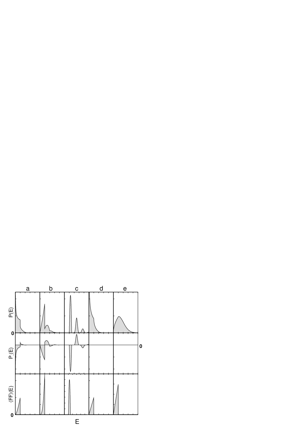
In Fig. 3, several different types of bath spectra $\left\langle\hat{F}\hat{F}\right\rangle_{E}$ are shown. Cases (a),(b),(d) and (e) are power-laws of the form given in Eq. (25), for a cutoff frequency of $\omega_{c}=1$. The last two (d,e) are of Ohmic type ($s=1,\,z=0$), which corresponds physically to gate voltage fluctuations due to Nyquist noise. Case (c) represents a bath with an excitation gap (for example optical phonons), with a spectrum given by an inverted parabola. In the limit of infinitely small spectral bandwidth, it would correspond to the single harmonic oscillator (Einstein mode) discussed above. Case (b), with a bath spectrum rising as $\omega^{3}$, corresponds to the experimentally relevant case of piezoelectric coupling to acoustic phonons, which was determined to be the major inelastic mechanism in the experiments of Ref. KouwenhouwenDD on double-dots in GaAs (see Ref. BrandesKramer for a theoretical analysis deriving this spectrum for wavelengths larger than the dot distance). The spectra for the first three cases (a,b,c) have been chosen to give the same renormalization factor, $z=1/e$. The same figure shows the resulting functions $P(E)$ and $P_{-}(E)$. These have been obtained using the integral equation described in Refs. minnhagen; ingoldhabil. We recall that the low-energy behaviour of $P(E)$ is given by $\left\langle\hat{\phi}\hat{\phi}\right\rangle_{E}=\left\langle\hat{F}\hat{F}\right\rangle_{E}/E^{2}$ for the cases with $z\neq 0$, where perturbation theory may be applied. In case (c), the alternating signs of the different contributions to $P_{-}(E)$ may be observed, whose physical meaning has been explained above for the limiting case of the harmonic oscillator.

We now briefly mention some numerical estimates for the bath strengths as they may occur in experimental situations.

In GaAs, the lack of inversion symmetry leads to piezoelectric fields proportional to the lattice deformation, whose effect on electrons at low frequencies is much stronger than that of the usual deformation potential (where it is only the potential that is proportional to the deformation). For the piezoelectric couplinggant to acoustic phonons in GaAs, one finds (compare Ref. BrandesKramer) $\left\langle\hat{\phi}\hat{\phi}\right\rangle_{\omega}^{T=0}=W\,\omega/(c_{s}/d)^{2}$ for $\omega\ll c_{s}/d$, where $c_{s}\approx 5\cdot 10^{3}\,m/s$ is an estimate for the average velocity of longitudinal sound waves in GaAs, and $d$ denotes the distance between the quantum dots. We obtain $W=const\cdot(eh_{14}/4\pi)^{2}/(\hbar\rho c_{s}^{3})$, where $eh_{14}=1.4\,eV/nm$ is the single piezo-electric modulus in the cubic $T_{d}$ structure of $GaAs$ and $\rho=5.3\cdot 10^{3}\,kg/m^{3}$ the mass density. The numerical constant is of order $1$ and accounts for the details of the sound wave dispersion relation as well as the orientation of the crystal axes with respect to the vector separating the quantum dots. Inserting these values, $W$ is found to be on the order of $0.01$. In order to obtain the renormalization factor $z$, the spectrum $\left\langle\hat{\phi}\hat{\phi}\right\rangle_{\omega}$ must be integrated over all frequencies (see above), i.e. up to the cutoff frequency $\omega_{c}$. The effective cutoff frequency $\omega_{c}\propto c_{s}/d_{0}$ is determined by the extent $d_{0}$ of the dot wave functions (for $d_{0}=100nm$ one obtains $\omega_{c}\sim 50\,GHz$). Given the present values, and assuming $d_{0}\approx d$, this leads to estimates for $\int\left\langle\hat{\phi}\hat{\phi}\right\rangle_{\omega}d\omega$ on the order of $0.01$, yielding $z=\exp(-\left\langle\hat{\phi}^{2}\right\rangle)$ near $1$. Note that the distance $d$ between the dots cancels in the estimate for $z$, as long as the cutoff frequency is assumed to be given by $\omega_{c}\propto c_{s}/d$. However, as $\omega_{c}$ might be considerably larger than $c_{s}/d$ (if $d_{0}\ll d$), one could also obtain a $z$ that deviates more strongly from unity.

For the Ohmic bath, we may imagine the quantum dots placed inside a capacitor $C$ connected to a circuit of resistance $R$, such that the potential difference $2\hat{F}$ between the dots would be given by the fluctuating voltage drop across the capacitor. This leads to a bath spectrum $\left\langle\hat{F}\hat{F}\right\rangle_{\omega}^{T=0}=\pi(R/R_{Q})\hbar^{2}\omega/(1+(RC\omega)^{2})$, with $R_{Q}=h/e^{2}$ the quantum of resistance. Therefore, the dimensionless coupling constant $\alpha$ introduced above would be equal to $\alpha=(\pi/2)R/R_{Q}$, which can have values both larger and smaller than $1$.

Finally, for optical phonons, we use the Fröhlich interaction Hamiltonian (Ref. mahan) with a dimensionless Fröhlich coupling constant of $\alpha=0.07$ (GaAs) to obtain the rough estimate $\left\langle\hat{F}\hat{F}\right\rangle_{\omega}^{T=0}=\delta(\omega-\omega_{LO})\cdot(1meV)^{2}\cdot(100nm/d_{0})$, with $\omega_{LO}\approx 5\cdot 10^{13}Hz$. This yields a $z$ deviating from unity by about $10^{-3}$.

However, in the plots we have chosen $z=1/e$ for illustrative purposes.

The resulting behaviour of $\Gamma(\varphi,V)$ at $T=0$, calculated from Eq. (13), is shown in Figs. 4 and 5. In the case of constructive interference ($\varphi=0$, Fig. 4), the decay rate for the “weak baths” (a,b,c) starts out from $\Gamma/2\Gamma_{0}=z$ at $V=0$ and goes to $\Gamma/2\Gamma_{0}=(1+z^{2})/2$ at $eV/\omega_{c}\gg 1$. The initial deviation from the constant value of $z$ at low voltages is given by the power-law $V^{2(s-1)}$ contained in Eq. (28). In contrast, the decay rate for the Ohmic bath (d,e) starts at $\Gamma=0$, rising with a power-law and saturating at a value of $\Gamma/2\Gamma_{0}=1/2$, corresponding to an equal admixture of odd and even states in the reduced density matrix of the electron coupled to the bath. For destructive interference ($\varphi=\pi$, Fig. 5), the behaviour of (a) and (b) at low voltages is given by $V^{s-1}$ (see Eq. (28)), while the decay rate of the Ohmic bath (d,e) remains the same as that for $\varphi=0$. In the special case (c) of the gapped bath, we observe perfect destructive interference up to the excitation threshold of the bath at $eV=\omega_{c}$, where $\Gamma(\varphi=\pi,V)$ increases in a stepwise manner for the first time, with the next increase at $eV=3\omega_{c}$. Note that, on the other hand, $\Gamma(\varphi=0,\,V)$ increases at even multiples of the excitation gap. The difference comes about because it is only the emission of an odd number of phonons into the bath that reveals the location of the electron, as discussed above. This feature would be absent if the two dots were coupled to two independent baths, whereas the other qualitative properties would remain the same.

From the decay rates at $\varphi=0$ and $\varphi=\pi$, we may calculate the visibility $\upsilon$ of the “interference pattern” that is defined by the dependence of $\Gamma$ on $\varphi$. The result is shown in Fig. 6. As we have noted before, the visibility is always zero for the Ohmic bath. On the other hand, for the “weak baths”, it is perfect (equal to $1$) at $V\rightarrow 0$, due to the perfect destructive interference, regardless of the suppression factor $z$ appearing in $\Gamma(\varphi=0)$. In general, the visibility decreases towards higher bias voltages before saturating at the limiting value of $z^{2}$. However, in contrast to intuitive expectation, the decrease may be nonmonotonous, i.e. the visibility of the interference effect may actually be enhanced by increasing the supply of energy available to the electron, although the decay rate $\Gamma$ always increases monotonously at any $V$. This is particularly striking in case (c), where the visibility drops down to zero in a certain range before rising again. The decrease down to the exact value of $0$ is related to the special choice of $\left\langle\hat{\phi}^{2}\right\rangle=1$ ($z=1/e$), which gives equal strengths of the peak at $E=0$ and the first peak around $E=\omega_{c}$, which then are able to cancel in the integral $\gamma_{-}$ over $P_{-}(E)$ that is proportional to the visibility. However, the physical reason for a dip in visibility is rather generic: In that energy range, the decay rate $\Gamma$ for $\varphi=\pi$ has already increased due to dephasing, while the blockade-type suppression of the value of $\Gamma$ for $\varphi=0$ has not yet been lifted. This is a consequence of the even-odd effect discussed above.

Up to now, we have discussed in detail the influence of the bath on the tunneling decay rate of an electron which has been placed onto the two dots in the symmetric superposition. In order to complete the picture, we have to calculate the sequential tunneling current through such a double-dot interference setup. This will be done by deriving and solving a master equation for the reduced density matrix of the double-dot system, taking into account the system-bath coupling exactly, while the tunnel-coupling is treated in leading order. We are interested specifically in the nonlinear response, i.e. in how an increasing bias voltage helps to destroy the phase coherence. The tunneling rates calculated previously will serve as input to the master equation.

However, in order to facilitate the understanding of the results, we first turn to a qualitative description of the situation without the bath.

At $\varphi=\pi$, tunneling is completely blocked, since the left reservoir only couples to the even state $\left|e\right\rangle$, while the right reservoir couples to the antisymmetric (odd) superposition, $\left|o\right\rangle$. At $\varphi=0$, both reservoirs couple to $\left|e\right\rangle$, whereas $\left|o\right\rangle$ is completely decoupled from the leads (compare the discussion in Ref. BoeseHofstetterSchoeller). This means that a current may flow if $\left|o\right\rangle$ is empty. However, if $\left|o\right\rangle$ is filled, the current vanishes, because double-occupancy is forbidden in our model. Since there is no way to change the occupation of $\left|o\right\rangle$, the stationary density-matrix of the double-dot at $\varphi=0$ will be any convex combination of these two possibilities (at $T=0$, in the absence of other relaxation paths). At any value of $\varphi$ in between these extremes, there is always the state $\left|\Psi\right\rangle=(\left|+\right\rangle-e^{-i\varphi}\left|-\right\rangle)/\sqrt{2}$, whose decay into the right lead is blocked by destructive interference. As there is a nonvanishing overlap between $\left|\Psi\right\rangle$ and the state $\left|e\right\rangle$ which is reached by tunneling from the left lead, one will observe an accumulation of population in $\left|\Psi\right\rangle$, until the current is blocked again. This argument holds at $T=0$, while at finite temperatures the electron can decay towards the left lead and make a new attempt. Therefore, in this simple picture, the stationary current at $T=0$ would be zero at any $\varphi$ except for $\varphi=0$, where it is undefined.

However, one has to take into account that the coupling to the reservoirs does not only lead to decay but also to an effective tunnel coupling between $\left|+\right\rangle$ and $\left|-\right\rangle$. Although this cannot change the blockade of the current at $\varphi=\pi$ (leading only to an energy shift of $\left|e\right\rangle$ vs. $\left|o\right\rangle$), it does lift the blockade at other values of $\varphi$. This is because the blocked state $\left|\Psi\right\rangle$ is no longer stationary, such that an electron will not remain there forever. The degeneracy at $\varphi=0$ still remains. Therefore, in the ideal case without coupling to a bath, we expect the current to vanish at $\varphi=\pi$ and to rise towards a maximal amplitude near $\varphi=0$. According to the previous argument, at $T=0$ this maximal amplitude will be determined by the effective tunnel-coupling between the dot states.

Introducing the bath will then lead to renormalization effects and spoil the perfect destructive interference at higher values of the bias voltage (or temperature), qualitatively in the same way as it has been explained above. We will show that the actual visibility $\upsilon_{I}$ of the current interference pattern $I(\varphi)$ is given by a monotonous function of the visibility $\upsilon$ introduced above for the tunneling rate (at symmetric bias).

We start with the Hamiltonian that is obtained after applying the unitary transformation of the independent boson model (79) onto our Hamiltonian (1):

Here $\epsilon^{\prime}$ is the (renormalized) energy of the two states, which we will take to be $\epsilon^{\prime}=0$ from now on. $U^{\prime}$ is the interaction constant that involves both the Coulomb repulsion as well as the effective attractive interaction induced by the bath. We assume $U,U^{\prime}\gg T,eV$, such that double-occupancy is forbidden.

The term which we will treat as a perturbation is given by $\hat{V}^{\prime}$, describing the tunneling to the left and the right leads in the presence of the bath. It is the transformed version of $\hat{V}$ (compare Eqs. (3) and (4) and Appendix A), where the additional fluctuating phase factors $\exp(\pm i\hat{\phi})$ have been introduced:

where

As usual, the current through the device does not only depend on the rates for electrons to tunnel into and out of the dots, but also on the stationary state which the system assumes in the nonequilibrium situation, i.e. under an applied bias voltage.

We will now derive a master equation for the reduced density matrix $\hat{\rho}$ of the double-dot system, which contains the populations $\rho_{++},\rho_{--},\rho_{00}$ (“$0$” denoting “no electron”) and the coherences $\rho_{+-}$ and $\rho_{-+}$ (with $\rho_{00}=1-\rho_{++}-\rho_{--}$, $\rho_{\alpha 0}=\rho_{0\alpha}=0$ for $\alpha\neq 0$, and $\rho_{-+}=\rho_{+-}^{*}$). We cannot simply use the standard kind of master equation, since we have to deal with two degenerate levels $\left|+\right\rangle$ and $\left|-\right\rangle$, and it is important that a tunneling event may create a coherent superposition of $\left|+\right\rangle$ and $\left|-\right\rangle$ (for example the even state $\left|e\right\rangle$). Such a master equation - for degenerate levels - has also been employed in Ref. koeniggefen (without coupling to the bath, and evaluated in the linear-response regime). The equation is different from that employed in the “orthodox” theory of sequential tunneling, where no coherent superpositions are involved. Note that for a finite tunnel-coupling the levels could be treated as degenerate as long as their energetic distance is much smaller than the level-broadening due to tunneling. However, as we consider the limit $\Gamma_{0}\rightarrow 0$, we need to have exactly equal energies. Otherwise, the energy of the hole that is created in the left electrode would betray the dot state which the electron has entered, thus preventing any coherent superposition to form.

Given the initial reduced density matrix $\hat{\rho}(0)$, and assuming the state of the environment (bath and reservoirs) to be independent of the electronic state on the dot at $t=0$, we obtain the time-evolution $\hat{\rho}(t)$ by tracing over the environmental degrees of freedom (“$E$”):

References

- (1) P. Mohanty, E. M. Q. Jariwala, and R. A. Webb, Phys. Rev. Lett. 78, 3366 (1997).
- (2) P. Cedraschi, V. V. Ponomarenko, and M. Büttiker, Phys. Rev. Lett. 84, 346 (2000).
- (3) P. Cedraschi and M. Büttiker, Phys. Rev. B 63, 165312 (2001); Annals of Physics, 289, 1 (2001).
- (4) A. D. Zaikin and D. S. Golubev, Physica B 280, 453 (2000).
- (5) F. Marquardt and C. Bruder, Phys. Rev. B 65, 125315 (2002).
- (6) K. E. Nagaev and M. Büttiker, Europhys. Lett. 58, 475 (2002).
- (7) F. Guinea, Phys. Rev. B 65, 205317 (2002).
- (8) D. S. Golubev, G. Schön, and A. D. Zaikin, cond-mat/0208548 (2002).
- (9) Y. Imry, cond-mat/0202044 (2002).
- (10) A. Stern, Y. Aharonov, and Y. Imry, Phys. Rev. A 41, 3436 (1990).
- (11) J. König and Y. Gefen, Phys. Rev. Lett. 86, 3855 (2001); Phys. Rev. B 65, 045316 (2002).
- (12) T. Fujisawa et al., Science 282, 932 (1998).
- (13) T. H. Stoof and Y. V. Nazarov, Phys. Rev. B 53, 1050 (1996).
- (14) Ph. Brune, C. Bruder, and H. Schoeller, Phys. Rev. B 56, 4730 (1997); Physica E 1, 216 (1997).
- (15) R. Ziegler, C. Bruder, and H. Schoeller, Phys. Rev. B 62, 1961 (2000).
- (16) T. Brandes and B. Kramer, Phys. Rev. Lett. 83, 3021 (1999).
- (17) R. Aguado and L. P. Kouwenhoven, Phys. Rev. Lett. 84, 1986 (2000).
- (18) S. Debald, T. Brandes, and B. Kramer, Phys. Rev. B 66, 041301 (2002).
- (19) M. Keil and H. Schoeller, cond-mat/0205308 (2002).
- (20) H. Akera, Phys. Rev. B 47, 6835 (1993).
- (21) T. V. Shahbazyan and M. E. Raikh, Phys. Rev. B 49, 17123 (1994).
- (22) A. W. Holleitner et al., Science 297, 70 (2002).
- (23) D. Boese, W. Hofstetter, and H. Schoeller, Phys. Rev. B 64, 125309 (2001).
- (24) D. Loss and E. V. Sukhorukov, Phys. Rev. Lett. 84, 1035 (2000).
- (25) M.-S. Choi, C. Bruder, and D. Loss, Phys. Rev. B 62, 13569 (2000).
- (26) D. Boese, W. Hofstetter, and H. Schoeller, Phys. Rev. B 66, 125315 (2002).
- (27) K. Haule and J. Bonca, Phys. Rev. B 59, 13087 (1999).
- (28) L. G. Mourokh, N. J. M. Horing, and A. Yu. Smirnov, Phys. Rev. B 66, 085332 (2002).
- (29) E. Buks et al., Nature 391, 871 (1998).
- (30) I. L. Aleiner, N. S. Wingreen, and Y. Meir, Phys. Rev. Lett. 79, 3740 (1997).
- (31) G.-L. Ingold and Y. V. Nazarov, in: Single Charge Tunneling, ed. by H. Grabert and M. Devoret, NATO ASI Series B, vol. 294, Plenum, New York (1992).
- (32) G. Schön, in: T. Dittrich et al., Quantum transport and dissipation, Wiley-VCH, Weinheim (1998).
- (33) G. D. Mahan: Many-Particle Physics, Plenum, New York (1981), pp. 269-310.
- (34) M. H. Devoret et al., Phys. Rev. Lett. 64, 1824 (1990).
- (35) P. Minnhagen, Phys. Lett. A 56, 327 (1976).
- (36) V. F. Gantmakher and Y. B. Levinson, Carrier scattering in metals and semiconductors, North-Holland, Amsterdam (1987), § 3.5.
- (37) K. Blum, Density Matrix Theory and Applications, Plenum, New York (1996).
- (38) H. Schoeller, Lect. Notes Phys. 544, 137 (2000). (cond-mat/9909400)
- (39) Y. Meir and N. Wingreen, Phys. Rev. Lett. 68, 2512 (1992).