On Design of Optimal Nonlinear Kernel Potential Function for Protein Folding and Protein Design

To model protein computationally, we first need a method to describe its geometric shape and its sequence of amino acid residues. Frequently, a protein is represented by a $d$-dimensional vector ${\mbox{\boldmath$c$}}\in{{{R}}}^{d}$. For example, we can represent a protein as a vector ${\mbox{\boldmath$c$}}\in{{{R}}}^{d}$, $d=20$, by measuring the solvent accessible surface areas of each of the 20 residue types. A method that is widely used is to count nonbonded contacts of various types of amino acid residue pairs in a protein structure. In this case, the count vector ${\mbox{\boldmath$c$}}\in{{{R}}}^{d},d=210$, is used as the protein descriptor. Once the structural conformation of a protein $s$ and its amino acid sequence $a$ is given, the protein description $f:({\mbox{\boldmath$s$}},{\mbox{\boldmath$a$}})\mapsto{{{R}}}^{d}$ will fully determine the $d$-dimensional vector $c$. In the case of contact vector, $f$ corresponds to the mapping provided by specific contact definition, e.g., two residues are in contact if their distance is below a specific cut-off threshold distance.

Based on the classical experiments of Anfinsen [41], a fundamental requirement for protein folding is that the native structure ${\mbox{\boldmath$s$}}_{N}$ with native amino acid sequence ${\mbox{\boldmath$a$}}_{N}$ must have an energy $H(f({\mbox{\boldmath$s$}}_{N},{\mbox{\boldmath$a$}}_{N}))$ that is the lowest among a set of alternative structure called decoys ${\cal D}=\{({\mbox{\boldmath$s$}}_{D},{\mbox{\boldmath$a$}}_{N})\}$, where the native amino acid sequence ${\mbox{\boldmath$a$}}_{N}$ takes a decoy conformation ${\mbox{\boldmath$s$}}_{D}$ that is different from the native conformation ${\mbox{\boldmath$s$}}_{N}$ [19, 42]:

Sometimes we can further require that the energy difference must be greater than a constant $b>0$:

A widely used functional form for protein potential function $H$ is the weighted linear sum of pairwise contacts [5, 6, 20, 21, 7, 8]. The linear sum energy $H$ is then:

As soon as the weight vector $w$ is specified, the potential function is fully defined. For such linear potentials, the basic requirement for protein potential is then:

or

if we require that the energy difference between a native structure and a decoy must be greater than a real value $b$.

There is a natural geometric view of the inequality requirement for weighted linear sum potentials. A useful observation is that each of the inequalities divides the space of ${{{R}}}^{d}$ into two halfs separated by a hyperplane. The hyperplane is defined by the normal vector $({\mbox{\boldmath$c$}}_{N}-{\mbox{\boldmath$c$}}_{D})$ and its distance $b/||{\mbox{\boldmath$c$}}_{N}-{\mbox{\boldmath$c$}}_{D}||$ from the origin. The weight vector $w$ must be located in the half-space opposite to the direction of the normal vector $({\mbox{\boldmath$c$}}_{N}-{\mbox{\boldmath$c$}}_{D})$ (Fig 1a). This half-space can be written as ${\mbox{\boldmath$w$}}\cdot({\mbox{\boldmath$c$}}_{N}-{\mbox{\boldmath$c$}}_{D})+b<0$.

When there are many inequalities to be satisfied simultaneously, the intersection of the half-spaces forms a convex polyhedron [43]. If the weight vector is located in the polyhedron, all the inequalities are satisfied. Potentials with such weight vector $w$ can discriminate the native protein from the set of all decoys.

For each native protein $i$, there is one convex polyhedron ${\cal P}_{i}$ formed by the set of inequalities associated with its decoys. If our potential can discriminate simultaneously $n$ structures from a union of sets of decoys, the weight vector $w$ must be located in a smaller convex polyhedron $\cal P$ that is the intersection of the $n$ convex polyhedra:

There is yet another geometric view of the inequality requirements. The relationship ${\mbox{\boldmath$w$}}\cdot({\mbox{\boldmath$c$}}_{N}-{\mbox{\boldmath$c$}}_{D})+b<0$ for all decoys and native protein structures can be regarded as a requirement that all points $\{{\mbox{\boldmath$c$}}_{N}-{\mbox{\boldmath$c$}}_{D}\}$ are located on one side of a hyperplane, which is defined by its normal vector $w$ and its distance $b/||{\mbox{\boldmath$w$}}||$ to the origin (Fig 1b). We can show that such a hyperplane exists if the origin is not contained within the convex hull of the set of points $\{{\mbox{\boldmath$c$}}_{N}-{\mbox{\boldmath$c$}}_{D}\}$ (see Appendix).

The second geometric view is dual and mathematically equivalent to the first geometric view. In the first view, a point ${\mbox{\boldmath$c$}}_{N}-{\mbox{\boldmath$c$}}_{D}$ determined by the structure-decoy pair $c_{N}=({\mbox{\boldmath$s$}}_{N},{\mbox{\boldmath$a$}}_{N})$ and $c_{D}=({\mbox{\boldmath$s$}}_{D},{\mbox{\boldmath$a$}}_{N})$ corresponds to a hyperplane representing an inequality, a solution weight vector $w$ corresponds to a point located in the final convex polyhedron. In the second view, each structure-decoy pair is represented as a point ${\mbox{\boldmath$c$}}_{N}-{\mbox{\boldmath$c$}}_{D}$ in ${{{R}}}^{d}$, and the solution weight vector $w$ is represented by a hyperplane separating all the points ${\cal C}=\{{\mbox{\boldmath$c$}}_{N}-{\mbox{\boldmath$c$}}_{D}\}$ from the origin.

Several optimization methods have been applied to find the weight vector $w$. The Rosenblantt perceptron method works by iteratively updating an initial weight vector ${\mbox{\boldmath$w$}}_{0}$ [21, 25]. Starting with a random vector, e.g., ${\mbox{\boldmath$w$}}_{0}={\bf 0}$, we test each native protein and its decoy structure. Whenever the relationship ${\mbox{\boldmath$w$}}\cdot({\mbox{\boldmath$c$}}_{N}-{\mbox{\boldmath$c$}}_{D})+b<0$ is violated, we update $w$ by adding to it a scaled vector $\eta\cdot({\mbox{\boldmath$c$}}_{N}-{\mbox{\boldmath$c$}}_{D})$. The final weight vector is therefore a linear combination of protein and decoy count vectors:

Here $\cal N$ is the set of native proteins, and $\cal D$ is the set of decoys. The set of coefficients $\{\alpha_{N}\}\cup\{\alpha_{D}\}$ gives a dual form representation of the weight vector $w$ as an expansion of the training examples, including both native and decoy structures.

If the final convex polyhedron $\cal P$ is non-empty, there can be infinite number of choices of $w$, all with perfect discrimination. But how do we find a weight vector $w$ that is optimal? This depends on the criterion for optimality. For example, one can choose the weight vector $w$ that minimizes the variance of energy gaps between decoys and natives: $\arg_{\mbox{\boldmath$w$}}\min\frac{1}{|{\cal D}|}\sum\left({\mbox{\boldmath$w$}}\cdot(c_{N}-c_{D})\right)^{2}-\left[\frac{1}{|{\cal D}|}\sum_{D}\left({\mbox{\boldmath$w$}}\cdot({\mbox{\boldmath$c$}}_{N}-{\mbox{\boldmath$c$}}_{D})\right)\right]^{2}$ as used in reference [20], or minimizing the $Z$-score of a large set of native proteins, or minimizing the $Z$-score of the native protein and an ensemble of decoys [44, 35], or maximizing the ratio $R$ between the width of the distribution of the energy and the average energy difference between the native state and the unfolded ones [18, 45]. A series of important works using perceptron learning and other optimization techniques [46, 18, 20, 21, 24] showed that effective linear sum potentials can be obtained.

Here we describe yet another optimality criterion according to the second geometric view. We can choose the hyperplane $({\mbox{\boldmath$w$}},b)$ that separates the points $\{{\mbox{\boldmath$c$}}_{N}-{\mbox{\boldmath$c$}}_{D}\}$ with the largest distance to the origin. Intuitively, we want to characterize proteins with a region defined by the training set points $\{{\mbox{\boldmath$c$}}_{N}-{\mbox{\boldmath$c$}}_{D}\}$. It is desirable to define this region such that a new unseen point drawn from the same protein distribution as $\{{\mbox{\boldmath$c$}}_{N}-{\mbox{\boldmath$c$}}_{D}\}$ will have a high probability to fall within the defined region, and non-protein points following a different distribution, which is assumed to be centered around the origin when no a priori information is available, will have a high probability to fall outside the defined region. In this case, we are more interested in modeling the region or support of the distribution of protein data, rather than estimating its density distribution function. For linear potential, regions are half-spaces defined by hyperplanes, and the optimal hyperplane $({\mbox{\boldmath$w$}},b)$ is the one with maximal distance to the origin. This is related to the novelty detection problem and single-class support vector machine studied in statistical learning theory [47, 36, 39]. In our case, any non-protein points will need to be detected as outliers from the protein distribution characterized by $\{{\mbox{\boldmath$c$}}_{N}-{\mbox{\boldmath$c$}}_{D}\}$. Among all linear functions derived from the same set of native proteins and decoys, the optimal weight vector $w$ is likely to have the least amount of mislabellings. The optimal weight vector $w$ can therefore be found by solving the following primal quadratic programming problem:

The solution maximizes the distance $b/||{\mbox{\boldmath$w$}}||$ of the plane $({\mbox{\boldmath$w$}},b)$ to the origin. The dual form of the same quadratic programming problem can be written as [48]:

where ${\mbox{\boldmath$x$}}_{i},{\mbox{\boldmath$x$}}_{j}\in\{({\mbox{\boldmath$c$}}_{N}-{\mbox{\boldmath$c$}}_{D})\}$.

However, it is possible that no such weight vector $w$ exists, i.e., the final convex polyhedron ${\cal P}=\bigcap_{i=1}^{n}{\cal P}_{i}$ may be an empty set. First, for a specific native protein $i$, there may be severe restriction from some inequality constraints, which makes ${\cal P}_{i}$ an empty set. Some decoys are very difficult to discriminate due to perhaps deficiency in protein representation. In these cases, it is impossible to adjust the weight vector so the native structure has a lower energy than the decoy. Second, even if a weight vector $w$ can be found for each native protein, i.e., $w$ is contained in a nonempty polyhedron, it is still possible that the intersection of $n$ polyhedra is an empty set, i.e., no weight vector can be found that can stabilize all native proteins against the decoys simultaneously. Computationally, the question whether a solution weight vector $w$ exists can be answered unambiguously in polynomial time [49], and recent studies using millions of decoys strongly suggest that when the number of native protein structure reaches 300–400, no such weight vector can be found [22, 20]. When perfect discrimination is impossible, a technique that minimizes the percentage of unsatisfied inequalities or the error rate was developed in reference [31].

A fundamental reason for this failure is that the functional form of linear sum of pairwise interaction is too simplistic. It has been suggested that higher order interactions such as three-body or four-body contacts should be incorporated [50, 51, 52]. Functions with polynomial terms using upto 6 degree of Chebyshev expansion has also been used to represent pairwise interactions [27].

Here we propose an alternative approach. At this time we still limit ourselves to pairwise contact interactions. We introduce a nonlinear potential function analogous to the dual form of the linear function in Equation (2), which takes the following form:

where $\alpha_{D}\geq 0$ and $\alpha_{N}\geq 0$ are parameters of the potential function to be determined, and ${\mbox{\boldmath$c$}}_{D}$ is a contact vector of decoy $D$ in the set of decoys $\cal D=\{({\mbox{\boldmath$s$}}_{D},{\mbox{\boldmath$a$}}_{N})\}$, ${\mbox{\boldmath$c$}}_{N}$ a contact vector of native structure $N$ in the set of native training proteins ${\cal N}=\{({\mbox{\boldmath$s$}}_{N},{\mbox{\boldmath$a$}}_{N})\}$. The difference of this functional form from linear function in Equation (2) is that a kernel function $K({\mbox{\boldmath$x$}},{\mbox{\boldmath$y$}})$ replaces the linear term. A convenient kernel function $K$ is:

Intuitively, the potential surface has smooth Gaussian hills of height $\alpha_{D}$ centered on the location ${\mbox{\boldmath$c$}}_{D}$ of decoy structure $D$, and has smooth Gaussian cones of depth $\alpha_{N}$ centered on the location ${\mbox{\boldmath$c$}}_{N}$ of native structures $N$. Ideally, the value of the potential function will be $-1$ for contact vectors ${\mbox{\boldmath$c$}}_{N}$ of native proteins, and will be $+1$ for contact vectors ${\mbox{\boldmath$c$}}_{D}$ of decoys.

To obtain the nonlinear potential, our goal is to find a set of parameters $\{\alpha_{D},\alpha_{N}\}$ such that $H(f({\mbox{\boldmath$s$}}_{N},{\mbox{\boldmath$a$}}_{N}))$ has energy value close to $-1$ for native proteins, and the decoys have energy values close to $+1$. There are many different choices of $\{\alpha_{D},\alpha_{N}\}$. We use an optimality criterion originally developed in statistical learning theory [37, 38, 39]. First, we note that we have implicitly mapped each structure and decoy from ${{{R}}}^{210}$ through the kernel function of $K({\mbox{\boldmath$x$}},{\mbox{\boldmath$y$}})=e^{-||{\mbox{\boldmath$x$}}-{\mbox{\boldmath$y$}}||^{2}/2\sigma^{2}}$ to another space with dimension as high as tens of millions. Second, we then find the hyperplane of the largest margin distance separating proteins and decoys in the space transformed by the nonlinear kernel. That is, we search for a hyperplane with equal and maximal distance to the closest native proteins and the closest decoys. Such a hyperplane can be found by obtaining the parameters $\{\alpha_{D}\}$ and $\{\alpha_{N}\}$ from solving the following Lagrange dual form of quadratic programming problem:

where $C$ is a regularizing constant that limits the influence of each misclassified conformation [47, 36, 37, 38, 39], and $y_{i}=+1$ if $i$ is a native protein, and $y_{i}=-1$ if $i$ is a decoy. These parameters lead to optimal classification of unseen test set proteins against decoys [47, 36, 37, 38, 39].

For protein sequence design, we assume that native sequence is more stable on the native conformation than on a different structure of another protein with low sequence identity. We use the method of gapless sequence threading to generate sequence decoys by mounting a sequence fragment from a different protein of a larger size of an unrelated structure to the native structure [19]. Because all native contacts are retained, we find that such sequence decoys are quite challenging.

For protein design, we seek potential functions that allows the search and identification of sequences most compatible with a specific given coarse-grain three-dimensional structure. We use a model analogous to the Anfisen experiments. We require that the native amino acid sequence ${\mbox{\boldmath$a$}}_{N}$ mounted on the native structure ${\mbox{\boldmath$s$}}_{N}$ has the lowest energy compared to a set of unrelated alternative sequences ${\cal D}=\{{\mbox{\boldmath$s$}}_{N},{\mbox{\boldmath$a$}}_{D}\}$ mounted on the same native protein structure ${\mbox{\boldmath$s$}}_{N}$:

Equivalently, the native sequence will have the highest probability to fit into the specified native structure. This is the same principle described in [53, 54, 55]. Much work has been done using linear design function of sum of contact pairs in the form of $H(f({\mbox{\boldmath$s$}},{\mbox{\boldmath$a$}}))=H({\mbox{\boldmath$c$}})={\mbox{\boldmath$w$}}\cdot{\mbox{\boldmath$c$}}$ [53, 54]. The discussion of the two geometric views of the weight vector of linear potential and the optimality criterion also applies to the sequence design problem.

We now explore nonlinear potential function for sequence design using the following functional form:

where $\alpha_{D}\geq 0$ and $\alpha_{N}\geq 0$ are coefficients to be determined, and ${\mbox{\boldmath$c$}}_{D}=f({\mbox{\boldmath$s$}}_{N},{\mbox{\boldmath$a$}}_{D})$ is the contact vector of a decoy sequence ${\mbox{\boldmath$a$}}_{D}$ mounted on its native protein structure ${\mbox{\boldmath$s$}}_{N}$, and ${\mbox{\boldmath$c$}}_{N}=f({\mbox{\boldmath$s$}}_{N},{\mbox{\boldmath$a$}}_{N})$ is the contact vector of a native sequence ${\mbox{\boldmath$a$}}_{N}$ from the set of native training proteins $\cal N$ mounted on the native structure ${\mbox{\boldmath$s$}}_{N}$. The only difference from nonlinear folding potential of Equation (3) is that here $\cal D$ is a set of sequence decoys mounted on native protein structures, rather than a set of structure decoys. Again, we use kernel function $K({\mbox{\boldmath$x$}},{\mbox{\boldmath$y$}})=e^{-||{\mbox{\boldmath$x$}}-{\mbox{\boldmath$y$}}||^{2}/2\sigma^{2}}$.

The optimal parameters $\{\alpha_{N}\}$ and $\{\alpha_{D}\}$ are obtained similarly by solving the following Lagrange dual convex quadratic programming problem:

where $C$ is a regularizing constant [37, 38], and $y_{i}=+1$ if $i$ is a native protein, and $y_{i}=-1$ if $i$ is a decoy.

Because protein molecules are formed by thousands of atoms, their shapes are complex. In this study we use the count vector of pairwise contact interactions derived from the edge simplices of the alpha shape of a protein structure. Edge simplices in the alpha shape represent nearest neighbor interactions that are in physical contacts. They encode precisely the same contact information as a subset of the edges in the Voronoi diagram of the protein molecule. These Voronoi edges are shared by two interacting atoms from different residues, but intersect with the body of the molecule modeled as the union of atom balls. We refer to references [56, 57] for further theoretical and computational details.

Maiorov and Crippen used the gapless threading method for generating a large number of structure decoys [19]. In this method, the sequence of a smaller protein ${\mbox{\boldmath$a$}}_{N}$ is threaded through the structure of an unrelated larger protein and takes the conformation ${\mbox{\boldmath$s$}}_{D}$ of a fragment of the larger protein [19]. Along the way, the sequence of the smaller protein can take the conformations of many fragments of the larger protein, each provides a structure decoy. With this approach, we generate for each native protein $\{({\mbox{\boldmath$s$}}_{N},{\mbox{\boldmath$a$}}_{N})\}$ a set of structure decoys $\{({\mbox{\boldmath$s$}}_{D},{\mbox{\boldmath$a$}}_{N})\}$ (Fig 2a).

We can generate sequence decoys in an analogous way, as already suggested in [42, 51]. In this case, we thread the sequence of a larger protein through the structure of a smaller protein, and obtain sequence decoys by mounting a fragment of the native sequence from the large protein to the full structure of the small protein. We therefore have for each native protein $({\mbox{\boldmath$s$}}_{N},{\mbox{\boldmath$a$}}_{N})$ a set of sequence decoys $({\mbox{\boldmath$s$}}_{N},{\mbox{\boldmath$a$}}_{D})$ (Fig 2b).

Following reference [22], we use protein structures contained in the Whatif database [58] in this study. Whatif database contains a representative set of sequence-unique protein structures generated from X-ray crystallography. Structures selected for this study all have pairwise sequence identity $<30\%$, R-factor $<0.21$, and resolution $<2.1$. Whatif database contains less structures than Pdbselect because the R-factor and resolution criteria are more stringent [58]. Nevertheless, it provides a good representative set of currently all known protein structures.

We use a list of 456 proteins compiled from the 1998 release (Whatif98) of the Whatif database [22], which was kindly provided by Dr. Vendruscolo. There are 192 proteins with multiple chains in this dataset. Some of them have extensive interchain contacts. For these proteins, it is possible that their conformations may be different if there are no interchain contacts present. We use the criterion of Contact Ratio to remove proteins that have extensive interchain contacts. Contact Ratio is defined here as the number of interchain contacts divided by the total number of contacts a chain makes. For example, protein 1ept has four chains A,B,C, and D. The intra chain contact number of chain B is 397. Contacts between chain A and chain B is 178, between B and C is 220, between B and other heteroatoms is 11. The Contact Ratio of chain B is therefore $(178+220+11)/(397+178+220+11)=51\%$. Thirteen protein chains are removed because they all have Contact Ratio $>30\%$. We further remove three proteins because each has $>10\%$ of residues missing with no coordinates in the Protein Data Bank file. The remaining set of 440 proteins are then used as training set for developing both folding and design potential functions. Using the sequence and structure threading method described earlier, we generated a set of 14 080 766 sequence decoys and a set of structure decoys of the same size.

For comparison, we develop optimal linear potential following the method and computational procedure described in reference[20]. We apply the interior point method as implemented in BPMD by Mészáros [59] to search for a weight vector $w$. We use two different optimization criteria as described in reference [20]. The first is:

where ${\mbox{\boldmath$w$}}_{i}$ denotes the $i$-th component of weight vector $w$, and $\epsilon=1\times 10^{-6}$. Let ${\cal C}=\{c_{N}-c_{D}\}$, and $|\cal C|$ the number of decoys. The second optimization criterion is:

We use SVMlight (http://svmlight.joachims.org/) [60] with Gaussian kernels and a training set of 440 native proteins plus 14 080 766 decoys to obtain the optimized parameter $\{\alpha_{N},\alpha_{D}\}$. The regularization constant $C$ takes default value, which is estimated from the training set ${{\cal N}\cup{\cal D}}$ as implemented in SVMlight:

Since we cannot load all 14 millions decoys into computer memory simultaneously, we use three heuristic strategies for training. In the first method, the total 14 080 766 decoys are divided randomly into 34 subsets. The training process starts with all native proteins and the first decoy set. After the training process converges, we select the decoy structures that have $\alpha_{i}\neq 0$ (these decoys are called support vectors [37, 38, 39]). From the second iteration on, we combined the native proteins, the new decoy set, and all decoys that appeared as support vectors in any of the previous training steps. These form the new training set for the next iteration of learning. This process is continued until all decoys have been exhausted in training.

In the second method, each of the 34 decoy subsets was combined with the native set in turn to form a training set. The decoy support vectors are then selected from each of the 34 training processes. All these decoy support vectors are combined, along with native proteins for a final training process. The results are taken as the optimized protein potential.

The third method is similar to the procedure reported in [20]. We first randomly selected a subset of decoys that fits into the computer memory. For example, we pick every 51st decoy from the list of 14 million decoys. This leads to an initial training set of 276 095 decoys and 440 native proteins. An initial protein potential is then obtained after learning. Next the energies for all 14 million decoys and all 440 native proteins are evaluated. Three decoy sets were collected based on the evaluation results: the first set of decoys contains the violating decoys which have lower energy than the native structures; the second set contains decoys with the lowest absolute energy, and the third set contains decoy support vectors identified in previous training process. The union of these three subsets of decoys are then combined with the 440 native protein as the training set for the next iteration of learning. This process is repeated until the energy difference to native protein for all decoys are greater than 0.0. Using this strategy, the number of iterations typically is between 2 and 10. During the training process, we set the cost factor $j$ in SVMlight to 120, which is the factor by which training errors on native proteins outweighs errors on decoys.

The value of $\sigma^{2}$ for the Gaussian kernel $K({\mbox{\boldmath$x$}},{\mbox{\boldmath$y$}})=e^{-||{\mbox{\boldmath$x$}}-{\mbox{\boldmath$y$}}||^{2}/2\sigma^{2}}$ is chosen by experimentation. We find that if the value of $\sigma^{2}$ is too large, no $\{\alpha_{N},\alpha_{D}\}$ can be found that can perfectly classifies the 440 training proteins and their decoys, i.e., the problem is unlearnable. If the value of $\sigma^{2}$ is too small, the performance in blind-test will deteriorate because of overfitting. For the 440 native proteins and the 14 080 766 sequence decoys, the value of $\sigma^{2}$ is chosen between 250.0 (for training method 1) and 138.9 (for training method 3). The final folding potential is obtained with $\sigma^{2}=227.3$ and the final design potential is obtained with $\sigma^{2}=138.9$, both derived using the third training method.

Using perceptron learning and a large number of decoys generated by gapless threading, Vendruscolo et al showed that if the number of native proteins exceeds 270, it is impossible to find parameters $w$ for potential function $H({\mbox{\boldmath$s$}},{\mbox{\boldmath$a$}})={\mbox{\boldmath$w$}}\cdot{\mbox{\boldmath$c$}}$, such that all native structures have lower energies than decoys [22]. That is, no $w$ can be found such that ${\mbox{\boldmath$w$}}\cdot{\mbox{\boldmath$c$}}_{N}<{\mbox{\boldmath$w$}}\cdot{\mbox{\boldmath$c$}}_{D}$ holds for all decoys.

Tobi et al showed that pairwise contact potential $H({\mbox{\boldmath$s$}},{\mbox{\boldmath$a$}})={\mbox{\boldmath$w$}}\cdot{\mbox{\boldmath$c$}}$ can be found to distinguish a different set of 572 proteins from a set of 28 213 009 structure decoys generated by gapless threading [20]. In this study, two residues are defined to be in contact if the geometric centers of their side chains are at a distance between 2.0 Å and 6.4 Å. To search for the optimal weight vector $w$, the authors used linear programming solver based on interior point method as implemented in BPMD by Mészáros [59].

We succeeded in reproducing the results of Tobi et al [20] and found a $w$ vector that enables perfect discrimination of the same set of 572 proteins used in [20] against 28 261 307 structure decoys we generated by gapless threading. We used the same contact definition based on Euclidean distance between geometric centers of side chains, as well as the same optimization criterion described earlier in the Methods section. The values of the 210 pairwise contact potentials (data not shown) are similar although not identical to the values listed in [20].

Structure decoys generated by gapless threading are obtained by taking a fragment of the structure of a large protein such that it contains exactly the same number of amino acid residues as the native protein. However, contacts in the resulting fragment structure often contain only a fraction of the total contacts in native protein.

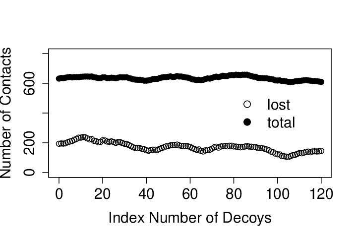
Design decoys are generated by taking a fragment sequence of a larger protein and thread it onto the native conformation of a smaller protein. As a result, although the contact count vector $c$ may be very different, the number of contacts in the design decoy is exactly the same as that in native protein. For decoys generated by gapless threading, design decoys therefore are far more challenge to discriminate then structure decoys (Fig 3).

Our experimentation confirms this observation. After generating 14 080 766 sequence design decoys for the 440 proteins in the training set, we apply the same interior point method to search for an optimal $w$ that can discriminate native sequences from decoy sequences. That is, we search for parameters $w$ for $H({\mbox{\boldmath$s$}},{\mbox{\boldmath$a$}})={\mbox{\boldmath$w$}}\cdot{\mbox{\boldmath$c$}}$, such that ${\mbox{\boldmath$w$}}\cdot{\mbox{\boldmath$c$}}_{N}<{\mbox{\boldmath$w$}}\cdot{\mbox{\boldmath$c$}}_{D}$ for all sequences. However, we fail to find a feasible solution for the weight vector $w$. This indicates that no $w$ exists capable of discriminating perfectly 440 native sequences from the 14 million decoy sequences. We repeated the same experiment using the set of 572 native proteins from reference [20] and 28 261 307 sequence decoys. The result is also negative.

To overcome the problems associated with linear potentials, we use the same set of 440 native proteins and 14 million decoys to obtain nonlinear kernel folding and design potentials. In both cases, we succeeded in finding a function in the form of Equation (3) that can discriminate all 440 native proteins from 14 million decoys.

Unlike statistical potentials where each native protein structure in the database contribute to the empirical potential, only a subset of native structures contribute and have $\alpha_{N}\neq 0$. In addition, a small fraction of decoys also contribute to the potential function. Table 1 list the details of the potential, including the numbers of native proteins and decoys that participate in Equation (3). These number represent about $60\%$ of native proteins and $<0.1\%$ of decoys from the original training data.

Blind test in discriminating native proteins from decoys using an independent test set is essential to assess the effectiveness of folding potentials. To construct a test set, we first take the entries in Whatif99 database that are not present in Whatif98. After eliminating proteins with chain length less than 46 residues, we obtain a set of 201 proteins. These proteins all have $<$ 30% sequence identities with any other sequence in either the training set or the test set proteins. Since 139 of the 201 test proteins have multiple chains, we use the same criteria applied in training set selection to exclude 7 proteins with $>30\%$ Contact Ratio or with $>10\%$ residues missing coordinates in the PDB files. This leaves a smaller set of test proteins of 194 proteins. Using gapless threading, we generate a sets of 3 096 019 structure decoys from the set of 201 proteins. This is a superset of the decoy set generated using 194 proteins.

For comparison, we also test the discrimination results of the optimal linear potential taken as reported in reference [20], as well as the statistical potential developed by Miyazawa and Jernigan. Here we use the contact definition reported in [20], that is, two residues are declared to be in contact if the geometric centers of their side chains are within a distance of 2.0 – 6.4 Å.

To test nonlinear folding potential functions for discriminating native proteins from structure decoys in both the 194 and the 201 test sets, we take the structure $s$ from the conformation-sequence pair $({\mbox{\boldmath$s$}},{\mbox{\boldmath$a$}}_{N})$ with the lowest energy as the predicted structure of the native sequence. If it is not the native structure ${\mbox{\boldmath$s$}}_{N}$, the discrimination failed and the folding potential does not work for this protein. The results of discriminating native structures using nonlinear folding potential are summarized in Table 2. There are 3 and 8 misclassified native structures for the 194 set and 201 set, respectively. These correspond to a failure rate of 1.5% and 4.0%, respectively. The optimal nonlinear kernel folding potential performs better than the optimal linear potential based on calculation using potential values taken as reported in reference [20] (failure rates 3.6% and 6.5% for the 194 set and 201 set, respectively). Consistent with previous reports [61], statistical potential has about $43.8\%$ (81 out of 194) and $43.2\%$ (87 out of 201) failure rates for the 194 set and the 201 set, respectively.

We use the same 194 set and 201 set of natives proteins and generate a set of 3 096 019 sequence decoys for testing the design potential. We take the sequence $a$ from the conformation-sequence pair $({\mbox{\boldmath$s$}}_{N},{\mbox{\boldmath$a$}})$ for a protein with the lowest energy as the predicted sequence. If it is not the native sequence ${\mbox{\boldmath$a$}}_{N}$, the discrimination failed and the design potential does not work for this protein.

Sequence decoys obtained by gapless threading are quite challenging, since all native contacts of the protein structures are maintained. No linear design potential function can be found using linear programming method that would succeed in the challenging task of identifying all 440 native sequences in the training set.

We succeeded in obtaining nonlinear design potential capable of discriminating all of the 440 native sequences (Table 3). It also works well in the test set. It succeeded in correctly identifying 92.8% (180 out of 194) of native sequences in the independent test set. This compares favorably with results obtained using optimal linear folding potential taken as reported in [20], which succeeded in identifying 80.9% (157 out of 194) of the test set, and the Miyazawa-Jernigan statistical potential (success rate 58.2%, 113 out of 194).

For the protein potentials derived with simple decoys generated by gapless threading, a more challenging test is to discriminate native proteins from an ensemble of explicitly generated three dimensional decoy structures with a significant number of near-native conformations [62, 7]. Here we evaluate the performance of nonlinear folding and design potential using three decoy sets from the database “Decoys ’R’ Us” [63]: the 4state_reduced set, the Lattice_ssfit set, and the lmsd set. We compare our results in performance with results reported in literature using optimal linear potential [64] and statistical potential [9] (Table 4). For the 4state_reduced set of decoys, nonlinear design potential has the best performance in terms of identifying the native structure. The only misclassified protein 1sn3 has three disulfide bonds, which are not modeled explicitly in the protein description of a vector in ${{{R}}}^{210}$. The correlation of root mean square distance of conformations to the native structure and energy value in the 4state set are shown in Fig 4. For proteins 1r69, 2cro, 3icb, and 1ctf, the correlation coefficient between the rmsd values and the energy values are good. We note that the nonlinear potential is obtained by learning from training decoys that are obtained by gapless threading. It is likely that nonlinear kernel potential can be further improved if more realistic structure decoys are included in training.

Because nonlinear potential is expressed as a kernel expansion of native protein and decoys, structure decoys and sequence decoys in general lead to different protein functions. For example, the contact count vectors $c$ can be very different for a sequence decoy of a protein and a structure decoy of the same protein. The potential surface defined by the folding potential and the design potential therefore may be different. There are 268 out of 440 native proteins participating in folding potential function with $\alpha$ value ranging from 0.01 - 28.04, of which 185 ($65\%$) are between 0.01 and 2.00. There are 347 out of 440 native proteins participating in design potential function, with $\alpha$ value ranging from 0.02 to 110.64, of which 269 ($77\%$) are between 0.02 and 2.00. Therefore, the majority of the native proteins have similar $\alpha$ values for both folding and design potentials. Fig 5 shows the difference $\Delta\alpha_{i}$ of the coefficient $\alpha_{i}$ for protein $i$ appearing in both folding potential and design potential. For the majority of the native proteins, $\Delta\alpha_{i}$ values are small. That is, most native proteins contribute similarly in design potential and in folding potential. This is expected, because the main differences between the two potentials are due to differences in decoy sets. The native proteins that contribute most differently to folding potential and design potential are small proteins. For example, there are 34 native proteins whose $|\Delta\alpha|>5.0$, and they all come from the top 100 smallest protein chains. Table 5 listed 20 proteins with highest $\alpha$ values for both kernel folding and design potentials. They are all small proteins and there are 15 out of the 20 proteins that appear both in folding and design potentials. It is possible that the energy values by kernel folding potential and by kernel design potential may be similar for many structure-sequence pairs $({\mbox{\boldmath$s$}},{\mbox{\boldmath$a$}})$. Figure 6a shows that the test 194 proteins have similar energy values by the kernel folding and kernel design potentials.

We also compare the energy value of the potential functions for each of the 210 unit vector ${\mbox{\boldmath$c$}}_{1}=\{1,0,\ldots,0\}^{T},\cdots$, and ${\mbox{\boldmath$c$}}_{210}=\{0,\ldots,1\}^{T}$. We normalize these values so $\max H({\mbox{\boldmath$c$}}_{i})=1$ for both potentials (Fig 7a). There is strong correlation ($R=0.91$) for folding and design potentials.

However, other methods reveal that kernel folding and design potentials are different. One method is to compare the energy values of a subset of decoy structures that are challenging. That is, we compare energies of decoys with $\alpha_{i}\neq 0$. Fig 7b shows that for decoys appearing in the design potentials, there is little correlation in energy values calculated by design potential and by folding potential. Similarly, there is no correlation between energy values calculated by folding potential and by design potentials for the set of structure decoys entering the design potential function (Fig 7c). It seems that although the values of $\alpha_{N}$s are similar for the majority of the native proteins, design potential and folding potential can give very different energy values for some conformations. This suggests that the overall fitness for design and folding potential may be somewhat different.

Potential functions derived from kernel models have the form of $H({\mbox{\boldmath$c$}})=\sum_{d\in\cal D}\alpha_{d}\cdot K({\mbox{\boldmath$c$}},{\mbox{\boldmath$c$}}_{d})-\sum_{N\in\cal N}\alpha_{n}\cdot K({\mbox{\boldmath$c$}},{\mbox{\boldmath$c$}}_{n})$, which cannot be directly compared with other potential functions of the form $H({\mbox{\boldmath$c$}})={\mbox{\boldmath$w$}}\cdot{\mbox{\boldmath$c$}}$. Here we follow the same approach as above and compare the energy values of the unit vectors, the native proteins, and the decoys using different potential functions. The energy values by nonlinear folding and design potentials have very little correlation with energy values evaluated using either optimal linear folding potential [20] or statistical potential [9] (Fig 6c-f). It seems nonlinear potentials developed in this work contains information absent in other potential functions.

References

- [1] Dill K, Bromberg S, Yue K, Fiebig K, Yee D, Thomas P, Chan H. Principles of protein folding–a perspective from simple exact models. Protein Sci 1995;4:561–602.
- [2] Levitt M, Gerstein M, Huang E, Subbiah S, Tsai J. Protein folding: the endgame. Annu Rev Biochem 1997;66:549–579.
- [3] Bonneau R, Baker D. Ab initio protein structure prediction: progress and prospects. Annu Rev Biophys Biomol Struct 2001;30:173–189.
- [4] Saven J. Designing protein energy landscapes. Chemical Reviews 2001;101:453–458.
- [5] Tanaka S, Scheraga H. Medium- and long-range interaction parameters between amino acids for predicting three-dimensional structures of proteins. Macromolecules 1976;9:945–950.
- [6] Miyazawa S, Jernigan R. Estimation of effective interresidue contact energies from protein crystal structures: quasi-chemical approximation. Macromolecules 1985;18:534–552.
- [7] Samudrala R, Moult J. An all-atom distance-dependent conditional probability discriminatory function for protein structure prediction. J Mol Biol 1998;275:895–916.
- [8] Lu H, Skolnick J. A distance-dependent atomic knowledge-based potential for improved protein structure selection. Proteins 2001;44:223–232.
- [9] Miyazawa S, Jernigan R. Residue-residue potentials with a favorable contact pair term and an unfavorable high packing density term. J Mol Biol 1996;256:623–644.
- [10] Wodak S, Rooman M. Generating and testing protein folds. Curr Opin Struct Biol 1993;3:247–259.
- [11] Sippl M. Knowledge-based potentials for proteins. Curr Opin Struct Biol 1995;5(2):229–235.
- [12] Lemer C, Rooman M, Wodak S. Protein-structure prediction by threading methods - evaluation of current techniques. Proteins 1995;23:337–355.
- [13] Jernigan R, Bahar I. Structure-derived potentials and protein simulations. Curr Opin Struct Biol 1996;6:195–209.
- [14] Simons KT, Ruczinski I, Kooperberg C, Fox B, Bystroff C, Baker D. Improved recognition of native-like protein structures using a combination of sequence-dependent and sequence-independent features of proteins. Proteins 1999;34:82–95.
- [15] Thomas P, Dill K. Statistical potentials extracted from protein structures: How accurate are they? J Mol Biol 1996;257:457–469.
- [16] Thomas P, Dill K. An iterative method for extracting energy-like quantities from protein structures. Proc Natl Acad Sci USA 1996;93:11628–11633.
- [17] Ben-Naim A. statistical potentials extracted from protein structures: Are these meaningful potentials? J Chem Phys 1997;107:3698–3706.
- [18] Goldstein R, Luthey-Schulten Z, Wolynes P. Protein tertiary structure recognition using optimized hamiltonians with local interactions. Proc Natl Acad Sci USA 1992;89:9029–9033.
- [19] Maiorov V, Crippen G. Contact potential that pecognizes the correct folding of globular proteins. J Mol Biol 1992;227:876–888.
- [20] Tobi D, Shafran G, Linial N, Elber R. On the design and analysis of protein folding potentials. Proteins 2000;40:71–85.
- [21] Vendruscolo M, Domany E. Pairwise contact potentials are unsuitable for protein folding. J Chem Phys 1998;109:11101–11108.
- [22] Vendruscolo M, Najmanovich R, Domany E. Can a pairwise contact potential stabilize native protein folds against decoys obtained by threading? Proteins 2000;38:134–148.
- [23] Bastolla U, Farwer J, Knapp E, Vendruscolo M. How to guarantee optimal stability for most representative structurs in the protein data bank. Proteins 2001;44:79–96.
- [24] Dima R, Banavar J, Cieplak M, Maritan A. Scoring functions in protein folding and design. Protein Sci 2000;9:812–819.
- [25] Micheletti C, Seno F, Banavar J, Maritan A. Learning effective amino acid interactions through iterative stochastic techniques. Proteins 20001;42(3):422–431.
- [26] Dobbs H, Orlandini E, Bonaccini R, Seno F. Optimal potentials for predicting inter-helical packing in transmembrane proteins. Proteins 2002;49(3):342–349.
- [27] Fain B, Xia Y, Levitt M. Design of an optimal Chebyshev-expanded discrimination function for globular proteins. Protein Sci 2002;11:2010–2021.
- [28] Vendruscolo M, Kussell E. Domany E. Recovery of protein structure from contact maps. Folding Design 1997;2:295–306.
- [29] Vendruscolo M, Domany E. Efficient dynamics in the space of contact maps. Folding Design 1998;3:329–336.
- [30] Skolni J, Kolinski A, Ortiz A. Monsster: a method for folding globular proteins with a small number of distance constraints. J Mol Biol 1997;265:217–241.
- [31] Xia Y, Levitt M. Extracting knowledge-based energy functions from protein structures by error rate minimization: Comparison of methods using lattice model. J Chem Phys 2000;113:9318–9330.
- [32] Koretke K, Luthey-Schulten Z, Wolynes P. Self-consistently optimized statistical mechanical energy functions for sequence structure alignment. Protein Sci 1996;5:1043–1059.
- [33] Koretke K, Luthey-Schulten Z, Wolynes P. Self-consistently optimized energy functions for protein structure prediction by molecular dynamics. Proc Natl Acad Sci U S A 1998;95(6):2932–2937.
- [34] Hao M, Scheraga H. How optimization of potential functions affects protein folding. Proc Natl Acad Sci U S A 1996;93(10):4984–4989.
- [35] Mirny L, Shakhnovich E. How to derive a protein folding potential? a new approach to an old problem. J Mol Biol 1996;264:1164–1179.
- [36] Vapnik V, Chervonenkis A. Theory of Pattern Recognition [in Russian]. Moscow: Nauka, 1974. (German Translation: W. Wapnik & A. Tscherwonenkis, Theorie der Zeichenerkennung, Akademie–Verlag, Berlin, 1979).
- [37] Vapnik V. The Nature of Statistical Learning Theory. N.Y.: Springer, 1995.
- [38] Burges CJC. A Tutorial on Support Vector Machines for Pattern Recognition. Knowledge Discovery and Data Mining 1998;2.
- [39] Schölkopf B, Smola A. Learning with kernels: Support vector machines, regularization, optimization, and beyond. Cambridge, MA: The MIT Press, 2002.
- [40] Meller J, Wagner M, Elber R. Maximum feasibility guideline in the design and analysis of protein folding potentials. J Comput Chem 2002;23:111–118.
- [41] Anfinsen C. Principles that govern the folding of protein chains. Science 1973;181:223–230.
- [42] Jones D, Taylor W, Thornton J. A new approach to protein fold recognition. Nature 1992;358:86–89.
- [43] Edelsbrunner H. Algorithms in combinatorial geometry. Berlin: Springer-Verlag, 1987.
- [44] Chiu T, Goldstein R. Optimizing energy potentials for success in protein tertiary structure prediction. Folding Des 1998;3:223–228.
- [45] Hao MH, Scheraga H. Designing potential energy functions for protein folding. Curr Opinion Structural Biology 1999;9:184–188.
- [46] Friedrichs M, Wolynes P. Toward protein tertiary structure recognition by means of associative memory hamiltonians. Science 1989;246:371–373.
- [47] Vapnik V, Chervonenkis A. A note on one class of perceptrons. Automation and Remote Control 1964;25.
- [48] Mangasarian O. Nonlinear programming. Philadelphia: SIAM Publishers, 1994.
- [49] Karmarkar N. A new polynomial-time algorithm for linear programming. Combinatorica 1984;4:373–395.
- [50] Betancourt M, Thirumalai D. Pair potentials for protein folding: Choice of reference states and sensitivity of predicted native states to variations in the interaction schemes. Protein Sci 1999;8:361–369.
- [51] Munson P, Singh R. Statistical significane of hierarchical multi-body potential based on delaunay tessellation and their application in sequence-structure alignment. Protein Sci 1997;6:1467–1481.
- [52] Zheng W, Cho S, Vaisman I, Tropsha A. A new approach to protein fold recognition based on Delaunay tessellation of protein structure. In: Altman R, Dunker A, Hunter L, Klein T, editors, Pacific Symposium on Biocomputing’97. Singapore: World Scientific, pp. 486–497, 1997; pp. 486–497.
- [53] Shakhnovich E, Gutin A. Engineering of stable and fast-folding sequences of model proteins. Proc Natl Acad Sci USA 1993;90:7195–7199.
- [54] Deutsch J, Kurosky T. New algorithm for protein design. Phys Rev Lett 1996;76:323–326.
- [55] Li H, Helling R, Tang C, Wingreen N. Emergence of preferred structures in a simple model of protein folding. Science 1996;273:666–669.
- [56] Edelsbrunner H. The union of balls and its dual shape. Discrete Comput Geom 1995;13:415–440.
- [57] Liang J, Edelsbrunner H, Fu P, Sudhakar P, Subramaniam S. Analytical shape computing of macromolecules I: Molecular area and volume through alpha-shape. Proteins 1998;33:1–17.
- [58] Vriend G, Sander C. Quality control of protein models - directional atomic contact analysis. J Appl Cryst 1993;26:47–60.
- [59] Mészáros C. Fast Cholesky factorization for interior point methods of linear programming. Comp Math Appl 1996;31:49 – 51.
- [60] Joachims T. Advances in Kernel Methods - Support Vector Learning, MIT Press. 1999; .
- [61] Clementi C, Maritan A, Banavar J. Folding, design, and determination of interaction potentials using off-lattice dynamics of model heteropolymers. Phys Rev Lett 1998;81:3287–3290.
- [62] Park B, Levitt M. Energy functions that discriminate x-ray and near-native folds from well-constructed decoys. J Mol Biol 1996;258:367–392.
- [63] Samudrala R, Levitt M. Decoys ‘R’ us: a database of incorrect conformations to improved protein structure prediction. Protein Sci 2000;9:1399–1401.
- [64] Tobi D, Elber R. Distance-dependent, pair potential for protein folding: Results from linear optimization. Proteins 2000;41:40–46.
- [65] Rossi A, Micheletti C, Seno F, Maritan A. A self-consistent knowledge-based approach to protein design. Biophys J 2001;80(1):480–490.