The Number of Attractors in Kauffman NetworksPreprint: LU TP 02-38
Abstract
The Kauffman model describes a particularly simple class of random Boolean networks. Despite the simplicity of the model, it exhibits complex behavior and has been suggested as a model for real world network problems. We introduce a novel approach to analyzing attractors in random Boolean networks, and applying it to Kauffman networks we prove that the average number of attractors grows faster than any power law with system size.
pacs
89.75.Hc, 02.70.UuI Introduction
We are increasingly often faced with the problem of modeling complex systems of interacting entities, such as social and economic networks, computers on the Internet, or protein interactions in living cells. Some properties of such systems can be modeled by Boolean networks. The appeal of these networks lies in the finite (and small) number of states each node can be in, and the ease with which we can handle the networks in a computer.
A deterministic Boolean network has a finite number of states. Each state maps to one state, possibly itself. Thus, every network has at least one cycle or fixed point, and every trajectory will lead to such an attractor. The behavior of attractors in Boolean networks has been investigated extensively, see e.g. Bornholdt and Sneppen 1998; Lemke et al. 2001; Bhattacharjya and Liang 1996; Bagley and Glass 1996; Fox and Hill 2001; Oosawa and Savageua 2002. For a recent review, see Aldana et al. 2002.
A general problem when dealing with a system is finding the set of attractors. For Boolean networks with more than a handful of nodes, state space is too vast to be searched exhaustively. In some cases, a majority of the attractor basins are small and very hard to find by random sampling. One such case is the Kauffman model Kauffman 1969. Based on experience with random samplings, it has been commonly believed that the number of attractors in that model grows like the square root of system size. Lately this has been brought into question Bastolla and Parisi 1997; Bastolla and Parisi 1998; Bilke and Sjunnesson 2001; Socolar and Kauffman 2002. Using an analytic approach, we are able to prove that the number attractors grows faster than any power law. The approach is based on general probabilistic reasoning that may also be applied to other systems than Boolean networks. The derivations in the analysis section are just one application of the approach. We have attempted to focus on the method and our results, while keeping the mathematical details at a minimum level needed for reproducibility using standard mathematical methods.
In 1969 Kauffman introduced a type of Boolean networks as a model for gene regulation Kauffman 1969. These networks are known as - models, since each of the nodes has a fixed number of inputs . A Kauffman network is synchronously updated, and the state (0 or 1) of any node at time step is some function of the state of its input nodes at the previous time step. An assignment of states to all nodes is referred to as a configuration. When a single network, a realization, is created, the choice of input nodes and update functions is random, although the update functions are not necessarily drawn from a flat distribution. This reflects a null hypothesis as good or bad as any, if we have no prior knowledge of the details of the networks we wish to model.
In this letter, we will first present our approach, and then apply it to Kauffman’s original model, in which there are 2 inputs per node and the same probability for all of the 16 possible update rules. These 16 rules are the Boolean operators of two or fewer variables: and, or, true, etc. This particular - model falls on the critical line, where the network dynamics is neither ordered nor chaotic Derrida and Pomeau 1986; Derrida and Stauffer 1986; Bastolla and Parisi 1997.
II Approach
Our basic idea is to focus on the problem of finding the number of cycles of a given length in networks of size . As we will see, the discreteness of time makes it convenient to handle cycles as higher-dimensional fixed point problems. Then it is possible to do the probabilistic averaging in a way which is suitable for an analytic treatment. This idea may also be expanded to applications with continuous time, rendering more complicated but also more powerful methods.
We use four key assumptions: (i) the rules are chosen independently of each other and of , (ii) the input nodes are independently and uniformly chosen from all nodes, (iii) the dynamics is dominated by stable nodes, and (iv) the distribution of rules is invariant due to inversion of any set of inputs. (iv) means e.g. that the fraction of and and nor gates are the same whereas the fraction and and nand gates may differ. (iv) is presumably not necessary, but simplifies the calculations drastically. (iii) is expected to be valid for any non-chaotic network obeying (i) and (ii) Flyvbjerg 1988. Note that (i) does not mean that the number of inputs must be the same for every rule. We could write a general treatment of all models obeying (i) – (iv), but for simplicity we focus on the Kauffman model.
We will henceforth use to denote the expectation value of the number of -cycles over all networks of size , with referring to fixed points. The average number of fixed points, , is particularly simple to calculate. For a random choice of rules, (i) and (iv) imply that the output state of the net is independent of the input state. Hence, the input and output states will on average coincide once on enumeration of all input states. This means that .
The problem of finding other -cycles can be transformed to a fixed point problem. Assume that a Boolean network performs an -cycle. Then each node performs one of possible time series of output values. Consider what a rule does when it is subjected to such time series on the inputs. It performs some boolean operation, but it also delays the output, giving a one-step difference in phase for the output time series. If we view each time series as a state, we have a fixed point problem. is then the average number of input states (time series), for the whole network, such that the output is the same as the input.
To take advantage of assumption (iv), we introduce the notion of -cycle patterns. An -cycle pattern is and inverted, where is a time series with period . Let denote a choice of -cycle patterns for the net, and let denote the probability that the output of the net is . Using the same line of reasoning as for fixed points, we conclude that (i) and (iv) yield
| (1) |
where is the set of proper -cycles of an -node net. A proper -cycle has no period shorter than .
III Analytic calculations
Assumption (ii) implies that is invariant under permutations of the nodes. Let denote the number of nodes expressing each of the patterns. For , we refer to as the pattern index. For convenience, let the constant pattern have index . Then
| (2) |
where denotes the multinomial and is the set of partitions of such that . That is, represents a proper -cycle.
What we have this far is merely a division of the probability of an -cycle into probabilities of different flavors of -cycles. Now we assume that each node has inputs. Then, we get a simple expression for that inserted into Eq. (2) yields
| (3) | |||||
where denotes the probability that the output pattern of a random 2-input rule has index , given that the input patterns have the indices and respectively. Note that Eq. (3) is an exact expression for the average number of proper -cycles in an -node random Boolean network which satisfies the assumptions (i), (ii), (iv), and where each node has inputs.
From now on, we only consider the Kauffman model, meaning that we also restrict the distribution of rules to be uniform. It is instructive to explore some properties of ; these will also be needed in the following calculations. We see that
| (4) |
for . Further, we note that for a given , has a non-zero value for exactly one . Let denote that value of . We can see as a function that rotates an -cycle pattern one step backwards in time. With this in mind we define . Now, we can write
| (5) |
for . ( is the Kronecker delta.)
We can view as a permutation on the set . Thus, we divide this index space into permutation cycles which are sets of the type . We refer to these permutation cycles as invariant sets of -cycles. Let denote the invariant sets of -cycles, where is the number of such sets. For convenience, let be the invariant set . If two -cycle patterns belong to the same invariant set, they can be seen as the same pattern except for a difference in phase.
We want to find the behavior of , for large , by approximating Eq. (3) with an integral. To do this, we use Stirling’s formula while noting that the boundary points where for some can be ignored in the integral approximation. Let for and integrate over . is implicitly set to . We get
| (6) |
where
| (7) |
Eq. (7) can be seen as an average , where is the expression inside the parentheses. Hence, the concavity of gives with equality if and only if
| (8) |
for all .
Note that Eq. (8) can be interpreted as a mean-field equation of the model. Using Eq. (8) for and Eq. (4) we see that comes arbitrarily close to zero only in the vicinity of , and for large , the relevant contributions to the integral in Eq. (6) come from this region. Thus, the dynamics of the net is dominated by stable nodes, in agreement with Flyvbjerg 1988; Bilke and Sjunnesson 2001. This means that assumption (iii) is satisfied by the Kauffman model. Using Eqs. (4) and (5), a Taylor-expansion of yields
| (9) | |||||
where .
The first order term of Eq. (9) has as its maximum and reaches this value if and only if for all . The second order term is zero at these points, while the third order term is less than zero for all . Hence, the first and third order terms are governing the behavior for large . Using the saddle-point approximation, we reduce the integration space to the space where the first and second order terms are . Let for and let denote the probability that the output pattern of a random rule belongs to , given that the input patterns are randomly chosen from and respectively. Thus, we approximate Eq. (6) for large as
| (10) |
where
| (11) | |||||
| (12) |
| (13) |
and . ( denotes the number of elements of the set .)
grows rapidly with . The number of elements in an invariant set of -cycle patterns is a divisor of . If an invariant set consists of only one pattern, it is either the constant pattern, or the pattern with alternating zeros and ones. The latter is only possible if is even. Thus, , with equality if is a prime number . Applying this conclusion to Eqs. (13) and (10), we see that for any power law , we can choose an such that grows faster than .
IV Numerical results

We have written a set of programs to compute the number of -cycles in Kauffman networks, Eq. (3), both by complete enumeration and using Monte Carlo methods, and tested them against complete enumeration of the networks with . The results for are shown in Fig. 1, along with the corresponding asymptotes. The asymptotes were obtained by Monte Carlo integration of Eq. (12). For low , is dominated by the boundary points neglected in Eq. (6), and its qualitative behavior is not obvious in that region.
A straighforward way to count attractors in a network is to simulate trajectories from random configurations and count distinct target attractors. As has been pointed out in Bilke and Sjunnesson 2001, this gives a biased estimate. Simulations in Kauffman 1969 with up to 200 trajectories per network indicated scaling with system size, whereas Bilke and Sjunnesson 2001 reported linear behavior with 1000 trajectories. That the true growth is faster than linear has now been firmly established Socolar and Kauffman 2002.
To closer examine the problem of biased undersampling, we have implemented the network reduction algorithm from Bilke and Sjunnesson 2001, and gathered statistics on networks with . We repeated the simulations for different numbers of trajectories , with . For each and , network realizations were examined, and we discarded configurations if no cycle was found within time steps. The results are summarized in Fig. 2a.
For , the number of attractors follows remarkably well, considering that gives the quite different behavior seen in Bilke and Sjunnesson 2001. If we extrapolate wildly from a log–loglog plot, fits the data rather well.
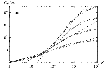
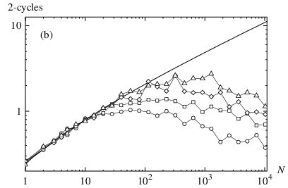
As another example of how severe the biased undersampling is, we have included a plot of the number of 2-cycles found in the simulations (Fig. 2b). The underlying distribution is less uniform than for the total number of attractors, so the errors are larger, but not large enough to obscure the qualitative behavior. The number of observed 2-cycles is close to for low , but as grows, a vast majority of them are overlooked. As expected, this problem sets in sooner for lower , although the difference is not as marked as it is for the total number of attractors.
V Summary
We have introduced a novel approach to analyzing attractors of random Boolean networks. By applying it to Kauffman networks, we have proven that the number of attractors in these grows faster than any power law with network size . This is in sharp contrast with the previously cited behavior, but in agreement with recent findings.
For the Kauffman model, we have derived an expression for the asymptotic growth of the number of -cycles, . This expression is corroborated by statistics from network simulations. The simulations also demonstrate that biased undersampling of state space is a good explanation for the previously observed behavior.
Acknowledgements.
We wish to thank Carsten Peterson, Bo Söderberg, and Patrik Edén for valuable discussions. This work was in part supported by the National Research School in Genomics and Bioinformatics.References
- Bornholdt and Sneppen (1998) S. Bornholdt and K. Sneppen, Phys. Rev. Lett. 81, 236 (1998).
- Lemke et al. (2001) N. Lemke, J. C. M. Mombach, and B. E. J. Bodmann, Physica A 301, 589 (2001).
- Bhattacharjya and Liang (1996) A. Bhattacharjya and S. Liang, Phys. Rev. Lett. 77, 1644 (1996).
- Bagley and Glass (1996) R. J. Bagley and L. Glass, J. Theor. Biol. 183, 269 (1996).
- Oosawa and Savageua (2002) C. Oosawa and M. A. Savageua, Physica D 170, 143 (2002).
- Fox and Hill (2001) J. J. Fox and C. C. Hill, Chaos 11, 809 (2001).
- Aldana et al. (2002) M. Aldana, S. Coppersmith, and L. Kadanoff (2002), submitted to Springer Applied Mathematical Sciences Series, eprint http://arXiv.org/abs/nlin.AO/0204062.
- Kauffman (1969) S. A. Kauffman, J. Theor. Biol. 22, 437 (1969).
- Bastolla and Parisi (1997) U. Bastolla and G. Parisi, J. Theor. Biol. 187, 117 (1997).
- Bastolla and Parisi (1998) U. Bastolla and G. Parisi, Physica D 115, 219 (1998).
- Bilke and Sjunnesson (2001) S. Bilke and F. Sjunnesson, Phys. Rev. E 65, 016129 (2001).
- Socolar and Kauffman (2002) J. E. S. Socolar and S. A. Kauffman (2002), submitted to Phys. Rev. Lett., eprint http://arXiv.org/abs/cond-mat/0212306.
- Derrida and Pomeau (1986) B. Derrida and Y. Pomeau, Europhys. Lett. 1, 45 (1986).
- Derrida and Stauffer (1986) B. Derrida and D. Stauffer, Europhys. Lett. 2, 739 (1986).
- Flyvbjerg (1988) H. Flyvbjerg, J. Phys. A 21, L955 (1988).