Dynamics of glassy systems
Abstract
These lecture notes can be read in two ways. The first two Sections contain a review of the phenomenology of several physical systems with slow nonequilibrium dynamics. In the Conclusions we summarize the scenario for this temporal evolution derived from the solution to some solvable models ( spin and the like) that are intimately connected to the mode coupling approach (and similar ones) to super-cooled liquids. At the end we list a number of open problems of great relevance in this context. These Sections can be read independently of the body of the paper where we present some of the basic analytic techniques used to study the out of equilibrium dynamics of classical and quantum models with and without disorder. We start the technical part by briefly discussing the role played by the environment and by introducing and comparing its representation in the equilibrium and dynamic treatment of classical and quantum systems. We next explain the role played by explicit quenched disorder in both approaches. Later on we focus on analytical techniques; we expand on the dynamic functional methods, and the diagrammatic expansions and resummations used to derive macroscopic equations from the microscopic dynamics. We show why the macroscopic dynamic equations for disordered models and those resulting from self-consistent approximations to non-disordered ones coincide. We review some generic properties of dynamic systems evolving out of equilibrium like the modifications of the fluctuation-dissipation theorem, generic scaling forms of the correlation functions, etc. Finally we solve a family of mean-field models. The connection between the dynamic treatment and the analysis of the free-energy landscape of these models is also presented. We use pedagogical examples all along these lectures to illustrate the properties and results.
1 Introduction
Graduate and undergraduate courses on statistical mechanics and thermodynamics are usually devoted to the theory of macroscopic systems in thermal equilibrium. In many experimental realizations, actually some of the more interesting ones at present, the situation is, however, very different. The systems are in contact with equilibrated environments but, for one reason or another, they do not manage to equilibrate with them. The systems evolve in time in an out of equilibrium manner.
The list of systems evolving out of equilibrium is very long. The reasons for not reaching equilibrium with the environment are also varied. The most common cases are those in which the time needed to equilibrate the sample falls beyond the experimental time-window. We discuss them in the context of domain growth, phase separation and classical and quantum glassy systems. Another important cause for lack of equilibration is the action of external forces that drive the samples out of equilibrium. In this context we discuss the rheological properties of glass forming liquids and glassy materials, that are closely related to the relaxation of the same systems. The driven dynamics of granular matter is another example of this kind. Finally, we briefly touch another type of problem that has received much attention in recent years: the relaxation and weakly driven dynamics of elastic manifolds in random potentials that model magnetic domain walls in disordered materials, superconductors, Wigner crystals, etc.
A common feature among the relaxing and weakly driven examples cited above is that they evolve very slowly. Thus, they belong to a particular class of the full set of non-equilibrium systems. Exploiting the fact that their dynamics is slow, and other more subtle properties that we shall discuss along these notes, we can hope to develop a common theoretical description for all of them.
In these lectures we focus on the study of a family of simple models that can be adapted to mimic the above mentioned physical systems. Typically, these models are fully connected interacting spin systems or models of interacting particles in infinite dimensions. They can be seen as the equivalent of the fully connected Ising model for ferromagnetism that correctly predicts the existence of a thermodynamic transition and the nature of the two phases but fails to describe the dependence on dimensionality or the precise critical behavior. Similarly, the schematic models do not include a notion of distance inside the system. This crude approximation allows one to solve the dynamics explicitly, paying the price of loosing information about the behavior in real space. Models of finite manifolds embedded in infinite dimensional spaces and under the effect of random potentials are generalizations of the schematic models that capture partial spatial information. They are also solvable analytically. Interestingly enough, one finds that these models realize several phenomenological approaches to glassy physics that have been known for long. Moreover, their dynamic macroscopic equations coincide with those arising from the self-consistent approximations used to analyze more realistic models as, for instance, the mode-coupling approach to super-cooled liquids. Having an exact solution is very important in many respects. Firstly, it establishes the phenomenological approaches on firmer bases. Secondly, it allows one to set clear limits of validity of the self-consistent approximations to realistic models. Thirdly, being defined by interacting potentials their free-energy density is accessible to analytical studies, from which one obtains the organization of metastable states and relates it to the dynamic properties. Fourthly, many important and common features of systems evolving slowly out of equilibrium have been discovered in the analytic solution to these models. Fifthly, one is able to identify some of the missing ingredients needed for a more accurate description of real systems. Even if their treatment has been too tough to implement correctly yet, it is important to know in which direction one could try improving the analytical study. In short, they constitute a very useful “laboratory” where one identifies general trends that can be later tested numerically and experimentally in more realistic models and real materials.
Although the models on which we concentrate are simple in the sense discussed above one needs to master many analytical methods to extract all the richness of their behavior. These methods are not completely standard and are not comprehensibly described in textbooks or lecture notes. For this reason, we try to present a rather complete and detailed introduction to them. We also discuss the scenario for glassy dynamics that stems out of this analysis. Finally, we mention several lines for future work that are currently being explored by several groups trying to go beyond the fully-connected and infinite dimensional models.
The lecture notes are organized as follows. In the next Section we introduce the phenomenology of the physical systems we are interested in paying special attention to the dynamic properties that we later describe analytically. The rest of the lecture notes are more technical. We start by reviewing very briefly several theoretical approaches to the glassy problem in Section 3. This summary is certainly not exhaustive but it may serve as a source of references. Since in the rest of the notes we shall develop classical and quantum systems in parallel we devote Section 4 to discuss how should one model the coupling between a system and its environment in both cases. In Section 5 we set the notation and we define several useful observables for spin and particle systems. The subject of Section 6 is a brief discussion of Fokker-Planck and Kramers processes and how they describe the approach to equilibrium. In the following Section we introduce the fluctuation-dissipation theorem, valid for systems evolving in equilibrium. Once these generic properties are established it will become simpler to discuss how they are modified in a system that evolves far from equilibrium. In Section 8 we explain the functional formalism that allows one to derive a generic dynamic effective action and the dynamic equations that we present in Section 9. We also introduce the very useful super-symmetric formulation of classical stochastic processes. In Section 10 we discuss an alternative method to obtain approximate dynamic equations. We focus on the mode-coupling (mc) approximation to show how averaging over disorder in some random models eliminates the same family of diagrams that the mc procedure neglects for non-disordered ones. The rest of the lectures are dedicated to the solution to the dynamic equations of the schematic models. We present it in as much generality as possible in Section 11. We discuss three generic results that were obtained when solving these equations without assuming equilibrium: the definition of correlation scales (Section 11.4), the modifications of the fluctuation-dissipation theorem (Section 13) and the definition of effective temperatures (Section 14). We also discuss how these properties appear in variations of the models that mimic the physical systems introduced in Section 2 and in finite toy models, simulations and experiments. Finally, in Section 15 we relate the dynamic results to the organization of metastable states via the static and dynamic approach of Thouless, Anderson and Palmer (tap). We briefly discuss the connection between it and the studies of the potential energy landscape (Edwards measure and inherent structure approach). Finally, in Section 16 we summarize the scenario for the glass transition and glassy dynamics derived from solvable mean-field models and present some of the lines for future research in this area.
2 Some physical systems out of equilibrium
In this Section we summarize the phenomenology of a number of systems with slow dynamics. We especially signal the features that we expect to capture with an analytical approach.
2.1 Domain growth
Out of equilibrium relaxational dynamics occurs, for instance, when one suddenly quenches a system with ferromagnetic interactions from its high temperature phase into its low temperature phase. When the system is in contact with a thermal bath at temperature ( is the Curie critical temperature) the system is disordered and the instantaneous averaged magnetization vanishes at all times. (The average refers here to a coarse graining over a region of linear size, , with and the correlation length.) All the one-time properties, such as the instantaneous averaged magnetization or the static magnetic susceptibility, can be computed using the Gibbs-Boltzmann distribution, . The system evolves in time but in a very simple manner controlled by . All properties of the equilibrium dynamics hold and any two-time correlation function is invariant under translations of time. Instead, if one externally and suddenly changes to set it below the Curie temperature, , the system evolves from the very disordered initial condition via the growth of domains of up and down magnetic order. With simple arguments one shows that the typical linear size of the domains grows as a power of the time spent in the low temperature phase, [1]. We call waiting-time, , the time spent since the entrance in the low- phase. The dynamic exponent depends on the kind of microscopic dynamics considered, e.g. for non-conserved order parameter while for conserved order parameter . All -dependence is concentrated in the prefactor . After the initial quench the system is a superposition of up and down domains and the magnetization averaged over the full system () vanishes. During coarsening domains grow. This is a scaling regime in which the system is statistically invariant under rescaling by the typical length . Typically, at a time the system orders and the averaged magnetization, , equals the magnetization of the conquering domain, say . Restricted ergodicity or equilibrium within one ergodic component holds in the sense that time and ensemble averages can be exchanged if and only if the time average is taken over a time window and the ensemble average is restricted to the configurations with positive magnetization. Since a rare fluctuation might lead the system to reverse from to another, still longer, characteristic time, , appears. This time is also a function of the size of the system and it is such that for times that are much longer than it complete ergodicity is restored. One can estimate it to be of Arrhenius type , with a constant, the dimension of space and the free-energy barrier to be surmounted to go from one ergodic component to the other.


The low temperature phase can also be reached with an annealing, e.g. by modifying the external temperature in steps of length and magnitude until reaching the working temperature . Since the entrance in the low- phase the system coarsens. If the prefactor increases with , after a time since crossing a system prepared with a slow cooling rate will have much larger structures than one of the same age that has been quenched into the ordered phase. The dynamics in isothermal conditions is basically identical in both cases but the starting configuration at the final temperature is however very different, the annealed system looking older than the quenched one. The presence or absence of cooling rate dependences as well as the effect of temperature on the low- dynamics allow one to distinguish among different glassy system. We shall come back to this issue when discussing structural and spin glasses.
On the right panel of Fig. 1 we plot the two-welled Landau free-energy density against . Transverse to the direction there are other directions that complete the phase space of the spin model. Note that when phase space is infinite dimensional even if real space is finite dimensional, . If one wishes to view the dynamics as the wandering of a point, that represents the instantaneous configuration of the system, in the free-energy landscape, the one-dimensional plot in Fig. 1 might be useful only if used carefully. The initial configuration after a quench corresponds to the top of the barrier (). This unstable point hides the , for , transverse directions ( is the lattice spacing). The domain growth process takes place while the representative point sits on the top of the barrier. Falling into one well corresponds to the growth of the conquering domain. Finally, jumping over the barrier is the activated process of reversing the full system. As long as the dynamics is highly non-trivial while viewed on this plot it looks trivial, with the representative point simply sitting on the border between the two basins of attraction of the equilibrium states [3].
Importantly enough, both and grow with and, if the thermodynamic limit is taken at the outset, diverging times with cannot be reached and physical times are always smaller than . The system cannot equilibrate with its environment and the non-equilibrium domain growth process goes on for ever.
2.2 Glasses
The domain growth example is very useful to visualize a non-equilibrium evolution. The mechanism behind the dynamics is clear and the growth of order can be easily identified. In other systems that undergo a non-equilibrium evolution whether there is a growing order controlling the evolution is still an open question. Glassy systems are one such example.
Understanding the glass transition and glassy dynamics is one of the greatest challenges in theoretical physics. The glassy problem can be summarized as follows [4]. Take a liquid at high temperature and quench it at a constant rate, . On each temperature step, the viscosity relaxes rather quickly and with a simple analysis one estimates its asymptotic value to trace a curve that is sketched in the left panel of Fig. 2 (red curve). This curve has several remarkable features. At very high temperature very slowly grows with decreasing . Decreasing the external temperature still the system approaches the crystallization (or melting) transition . If the cooling rate is sufficiently fast, this transition is avoided and the system enters a metastable super-cooled liquid phase where the viscosity grows very quickly with decreasing . Indeed, one typically observes that when changes by, say, , the viscosity jumps by approximately orders of magnitude. In consequence, the dynamics of the liquid slows down enormously. For several liquids the form of the curve can be described with a Vogel-Fulcher law,
| (2.1) |
that predicts a divergence of when . These liquids are conventionally called fragile. (Within the experimental precision coincides with the Kauzmann temperature where the extrapolation of the difference between the entropy of the liquid and the crystal vanish.) However, this fitting procedure can be criticized for several reasons. In many cases the form of the fitting function strongly depends on the temperature window chosen for the fit. Even more important is the fact that the dynamics becomes so slow when decreases that the time needed to equilibrate the sample goes beyond the minimal cooling rate, or the maximum time reachable in the experience. Below a temperature one can no longer equilibrate the sample. One of the most clear signatures of the absence of equilibrium below is the fact that the measurement of, e.g., the volume as a function of temperature, depends on the cooling rate, , used to reach . Moreover, decreases with decreasing cooling rate. Hence, the so-called “glass transition” is not a true thermodynamic transition but a dynamic crossover from the super-cooled liquid phase, where the dynamics is slow but occurs as in equilibrium [5], to the glass phase where the system does not manage to equilibrate with its environment. These features are schematically shown in the right panel of Fig. 2. Going back to the interpretation of Eq. (2.1), some authors extrapolate it below , where viscosity measurements are not possible, and interpret the divergence at as the signature of a true thermodynamic transition. This means that even in the limit of vanishing cooling rate one would observe a transition from the super-cooled liquid to an ideal glass phase (still metastable with respect to the crystal) at . Others prefer a scenario in which Eq. (2.1) has no meaning below .


In this sense, it is important to stress that the viscosity of many glass forming liquids, as the silica materials that give rise to window glass, is well fitted by an Arrhenius law
| (2.2) |
that diverges at . These are the so-called strong glasses. It has been suggested that actually all glasses are strong since one can always fit with an Arrhenius law if the temperature window used for the fit is close enough to (as suggested in Fig. 2). This is the reason why some authors prefer a scenario in which the super-cooled liquid phase extends all the way up to when an infinitely slow cooling rate is used. The curve labeled mct in the same figure shows the prediction of the models we shall discuss in these notes ( spin models and mode-coupling theory). In short, this approach predicts a dynamic transition at that is typically higher than , with a power law divergence of . Albeit this and other defects, this approach is successful in many respects since it yields a satisfactory qualitative description of the phenomenology of super-cooled liquids and glasses.
For the purpose of our discussion the important point to stress is the fact that the liquid falls out of equilibrium at the (cooling rate dependent) temperature . Indeed, even the “state” reached by the system below depends on the cooling rate as seen, for instance, in measurements of volume, entropy, etc. as functions of , see the right panel in Fig. 2. The slower the cooling rate, the deeper one penetrates below the threshold level corresponding to . The dynamics below occurs out of equilibrium since , see the sketch in Fig. 3. The properties of the system cannot be described with the use of and a more sophisticated analysis has to be developed.

The above paragraphs were devoted to the discussion of the liquid to glass transition and it implicitly assumed that the system was made of molecules in interaction. In the case of simple liquids, in which the constituents have no structure, one can describe the relevant interactions with a two body potential
| (2.3) |
Hard spheres are the simplest example of this kind where the only interaction are hard core ones that forbid the penetration of one particle by another. Adding polymers in the solution that hosts the spheres one can tune a repulsive interaction between the particles. (See Fig. 4-left below for a snapshot of one such experimental system [6].) Favorite potentials used in numerical simulations are the Lennard-Jones and soft-sphere ones
| (2.4) |
To avoid crystallization one usually uses a binary system with particles with mass and particles with mass . The parameter fixes the length scale, the energy scale and the mass scale. The time scale is then given by . For a given density, e.g. , an adequate choice of the remaining parameters yields the expected properties of a liquid or a glass with a numerical transition at a temperature where the relaxation time goes beyond the time accessible with the simulation. In the soft-sphere model one only keeps the repulsive term in the potential. Many other types of glasses are known in Nature. For instance, plastics as PVC whose mesoscopic constituents are polymers also undergo a glass transition very similar to the one described previously. Several types of interactions between the monomers that form the macromolecules are also of two-body type and they are repertoriated in the literature. The dynamics of particle systems is given by Newton’s equations.
2.3 Spin-glasses
More exotic types of glasses have been studied for long. Spin-glasses have attracted the attention of experimentalists and theoreticians as a prototypical system with quenched disorder [7, 8, 9, 10]. These systems are magnetic alloys in which magnetic impurities are replaced in a magnetically inert host. The impurities occupy random positions and are not displaced within the sample in experimental times. The interactions between the impurities depend on the distance between them. Since the latter are random, the interactions themselves take random values that change in sign very quickly. A number of experimental realizations exist. As in other glassy systems, spin-glasses fall out of equilibrium at a transition temperature when usual cooling rate procedures are used. From experimental and numerical results near complemented with standard critical analysis, it is rather generally believed that the transition between the paramagnetic and the spin-glass phase is, in this case, a true thermodynamic transition. This is at variance with what occurs in structural and polymeric glasses. Another important difference with structural glasses and systems undergoing simple coarsening as ferromagnets is that the magnitude of cooling rate dependences is quite negligible suggesting that for spin-glasses the preferred configurations at one temperature are totally different from the ones at any other temperature. Still, slightly farther away from the transition one can no longer equilibrate the spin-glasses and observes typical non-equilibrium effects.


Edwards and Anderson proposed a simplified model for spin-glasses in which one represents the magnetic impurities with Ising spins placed on the vertices of a three dimensional cubic lattice. The random nature of the interactions are mimicked with first neighbors random interactions between the spins taken from a Gaussian (or bimodal) probability distribution with zero mean and variance where is the connectivity of the lattice. (Hereafter we denote with square brackets the average over disorder.) The Hamiltonian is
| (2.5) |
where the vector encodes the full set of spins in the sample and represents nearest neighbors on the lattice. In the fully connected limit in which each spin interacts with all others the sum runs over all pair of spins and the unusual normalization of the s, , ensures a correct thermodynamic limit. This is the Sherrington - Kirkpatrick (sk) model
For many years it was common lore that the presence of explicit quenched disorder made spin-glasses intrinsically different from glasses where no quenched random forces have been identified. This belief was in part motivated by the analytical treatment used to study the equilibrium properties of the spin-glass phase in sk, namely, the replica trick. More recently, after a series of seminal papers by Kirkpatrick, Thirumalai and Wolynes [11], and the later solution to the non equilibrium dynamics of several glassy models [12, 13], it has been realized that the presence of quenched disorder is not that relevant. All glasses can be analyzed on the same footing. The schematic mean-field model for glasses, the spin model, has quenched Gaussian interactions and its Hamiltonian is
| (2.6) |
( and , we henceforth set .) Glauber’s rule for Ising spins or Langevin equations for soft spins define the microscopic evolution.
2.4 Quantum fluctuations
Different driving dynamics slightly modify the picture just presented. Quantum glassy phases, where quantum fluctuations are at least as important as thermal activation, have been identified in a number of materials. Two such examples are the spin glass compound and the amorphous insulator studied in [14] and [15], respectively. Another interesting realization is the so-called Coulomb glass in which localized electrons interact via Coulomb two-body potentials and hop between localization centers [16]. In all these systems the dynamics is extremely slow and strong history dependence as well as other glassy features have been observed.
Models for magnetic compounds are constructed with spins while models for particle systems are quantized with the usual commutation relations between coordinate and momenta. In both cases the dynamics is fixed by Heisenberg equations.
2.5 Rheology and granular matter


The above examples concern systems that are not able to reach equilibrium with their environments in a reasonable time but that, let evolve on astronomical time-scales, will eventually equilibrate. Other ways of establishing non-equilibrium states with slow dynamics are possible if one externally drives the samples [17].
A dense liquid can be driven to a slow out of equilibrium stationary regime by a weak shear. A shear is an example of a force that does not derive from a potential, i.e. it cannot be written as . The simplest way to apply a shear on a liquid is by means of a rheometer. In Fig. 5 we show one with a Couette geometry. The shear modifies the dynamic equations for the fluid by adding an advection . In the planar limit where is the velocity of the fluid, its density and the shearing rate. One mimics such a force in a spin system with a non-symmetric force, i.e. the force exerted by the spin on the spin is not equal to the force exerted by the spin on the spin [18, 19], e.g.
| (2.7) |
(The motivation to define such a force comes from neural nets where the synapsis have a direction.) It is clear that this force cannot be written as the variation of a potential energy with respect to , it violates detail balance, and an equilibrium measure cannot describe its effects [20].
A weak shear has a spectacular effect on the relaxation of liquids [21]. Usually, the viscosity as a function of the shear rate, , has a Newtonian plateau at small that crosses over to a decreasing function that is approximately given by . Hence, by shearing the liquid one facilitates its flow and the relaxation time decreases with increasing . Moreover, one introduces a shear-dependent time scale that plays an important role in aging experiments as discussed in Section 2.7.
Another family of materials that have captured the attention of experimentalists and theoreticians in recent years is granular matter [22]. Since the potential energy needed to displace a macroscopic grain by a distance equal to its diameter, , is much larger than the characteristic thermal energy, , thermal activation is totally irrelevant for systems made of macroscopic grains. Therefore, in the absence of external driving granular matter is blocked in metastable states and there exists no statistical mechanics approach capable of describing its static behavior. Instead, when energy is pumped in in the form of shearing, vibration or tapping, transitions between the otherwise metastable states occur and granular matter slowly relaxes towards configurations with higher densities. When trying to model these systems it is also important to keep in mind that dissipation is not given by the usual Ohmic form proportional to the velocity of the grains, , but it is much more cumbersome. Glassy features such as hysteresis as a function of the amount of energy injected, slow dynamics [22], and non stationary correlations [23, 24, 25] have been exhibited.
2.6 Elastic manifolds in random potentials
The motion of a dimensional directed elastic manifold embedded in an dimensional space in the presence of quenched random disorder has a bearing in several areas of physics [27, 28]. (The total dimension of space is .) The case represents a particle in a random potential. With , and an attractive punctual disorder one models, for instance, a single vortex in a dirty superconductor. When and one describes the dynamics of a directed interface in three dimensions. The standard model is
| (2.8) |
where and represents the transverse position of the point on the manifold and is a Gaussian random potential, with zero mean and correlations .
The study of these problems has been boosted by the advent of high- superconductivity. Other physical systems that are modeled with similar Hamiltonians are Wigner crystals, vortex lattices, charge density waves, etc. in the presence of disorder. All these problems have an underlying periodic structure that is modified by elastic distortions, topological defects and external quenched disorder. They can be set into motion with an external force and the velocity-force characteristics has several interesting features that have been much studied. One observes a depinning transition at , creep dynamics when the applied force is weak and , hysteresis, etc. (The driven motion is achieved, for instance, by applying an external current in the case of the vortex systems and the current-voltage characteristics is monitored.) The relaxational and driven dynamics of these systems show similarities but also marked differences with that of glasses and spin-glasses that are possibly due to the existence of an ordered underlying structure.
2.7 Aging
Aging means that older systems relax in a slower manner than younger ones [29]. One defines the age of a system as the time spent in the phase under study. For instance, the age of a system that is suddenly quenched from high- to low- is simply . The aging properties are studied by monitoring the time evolution of correlation and response functions. In the former experiments one lets the system evolve and compares its configuration at the waiting-time with the one reached at the subsequent time . In the latter one perturbs the system at with, e.g. a dc or an ac field, and follows the evolution of the linear response to the perturbation. In the glassy phase both correlations and responses depend on in an aging manner and, within the experimentally accessible time-window, this trend does not show any tendency to stop. At temperatures that are close but above one observes “interrupted aging”, that is, a dependence on the age of the system until it reaches the equilibration time () where the dynamics crosses over to an equilibrium one. In equilibrium correlation and response measurements are related in a system independent manner by the fluctuation-dissipation theorem (see Section 7). Out of equilibrium this general relation does not hold and, as we shall explain in Sections 13 and 14, important information can be extracted from its modifications.
Aging has an easy interpretation within coarsening systems. While the averaged domain size grows with , its rate of increase decreases, e.g. in the example explained in Section 2.1. The motion of interfaces slows down as time elapses. Comparing the configuration at and at a later time , one finds a clear separation of time-scales depending on the relative value of with respect to . If , one has , and the domain walls do not move. The overlap between the configurations at and is a sum of overlaps between domains of one and another type. (This holds when the ratio between the number of spin in the surface of the domains and in the bulk vanishes in the thermodynamic limit. Some non-standard systems have fractal scaling of the interfaces and the volume of the domains might also have a fractal dimensionality [30].) Due to thermal fluctuations within the domains, the correlation decays as in equilibrium from at equal times to when increases while still satisfying the constraint . For ’s beyond this limit, the correlations decay below since the interfaces move and one compares configurations with very different domain structures as shown, for instance, in the two snapshots in Fig. 1.
In structural glasses, a pictorial explanation of aging is also possible imagining that each particle sees a cage made of its neighbors. When is short compared to a characteristic time each particle rapidly rattles within its cage and the decorrelation is only characterized by thermal fluctuations. The correlations decay in a stationary manner from its value at equal times to a value called that will be defined precisely in Section 12 [in the domain growth example ]. When increases, the motion of the particles destroys the original cages and one sees the structural relaxation. The waiting-time dependence implies that the cages are stiffer when time evolves. The motion of a tagged particle is depicted in the left panel of Fig. 4 [6]. One sees how it first rattles within a cage to later make a long displacement and start rattling within another cage.
In spin-glasses no consensus as to which is the origin of aging has been reached. Still, the qualitative behavior of correlations and responses is rather close to the one in domain growth and structural glasses. In Fig. 6 we show the decay of the thermoremanent magnetization (an integrated linear response) and the correlations between the fluctuations of the magnetization in a spin-glass [31, 32].
Shearing may have a very strong effect on an aging system. In some cases it introduces a characteristic time that yields the longest relaxation time. Thus, aging is interrupted for waiting-times that are longer than (see Fig. 7). This effect has been known for long experimentally [21] and it has been found and explored recently within the theoretical framework that we review [33, 34]. Experiments in other soft glassy materials with aging and aging interrupted by shear can be found in [35]. Some examples where the effect of shearing is not as spectacular are also known. For instance, in a phase separating mixture sheared in one direction the domains stop growing in the transverse direction while they continue to grow longitudinally (see [19] and references therein). This is a subject of intensive research.
Granular matter is usually driven with periodic forces or tapping. These perturbations pump energy into the system that is evacuated via friction and introduce a time-scale that is simply the period of the oscillation. How these forces influence the aging properties is much less known and it is the subject of current investigations. For the moment, most of the work in this direction has been numerical [24, 25] and also analytical within the kind of models we shall solve [26] (see [23] for some experimental studies).
The aging properties of relaxing manifolds in random potentials have been found analytically [36] and numerically [37]. The experiment of Portier et al [38] shows aging features in a high- superconductor [39] that are also observed numerically [40, 41]. However, other experimental studies using different protocols have not exhibited these properties [42]. More experiments are needed to get a better understanding of the non-equilibrium relaxation of these systems. An external electric current drives a vortex system in its transverse direction due to Lorentz forces. How the longitudinal and transverse aging properties of the system are modified in the moving phases is another problem that deserves further study [43]. The comparison between the dynamics of the moving vortex lattice, the tapped dynamics of granular matter and the sheared dynamics of dense liquids is also interesting and begins to be done.


2.8 Summary
In this Section we introduced several examples of macroscopic systems that evolve with a slow non-equilibrium macroscopic dynamics. The microscopic dynamics governing the evolution of the constituents of each system is very different. For systems undergoing domain growth and classical glasses, is the external control parameter that generates fluctuations. For glasses at very low thermal fluctuations are almost completely irrelevant while quantum fluctuations become important and drive the dynamics. For granular matter is again irrelevant and the systems’ relaxation is due to the external drive. In the elastic systems an underlying ordered structure is visible and may cause important differences in the macroscopic dynamics with respect to other glassy systems where no quasi order has been identified. An ubiquitous phenomenon in these slowly evolving systems out of equilibrium is (sometimes interrupted) aging or the breakdown of stationarity. Even if all these systems seem to be totally different, a common formalism to study their macroscopic dynamics is now being used and a common picture starts to develop.
In the rest of these lectures we shall explain the main technical tools needed to study simplified models for these real systems. We shall describe the main features of the out-coming scenario making contact with the phenomenology introduced in this Section.
3 Theoretical approach
Besides many phenomenological descriptions of the glass transition and glassy dynamics proposed long ago, recently, several theoretical approaches have been developed. In the following we briefly describe some of the main ones.
Dynamics in the phase space.
The instantaneous configuration of the full system is a point in phase space that moves as time goes on (see the right panel in Fig. 1). In a whole family of models one assumes a free-energy landscape on phase space with wells and barriers and proposes that the point evolution is given by some dynamic prescription on this space. Choosing a convenient distribution and organization of wells and barriers, aging effects are captured by such models. (An average over different systems or over different parts of the same system is implicitly assumed in order to obtain smooth results for the observables.) In “trap models”, for instance, each well has an associated trapping-time such that once the system falls in the trap it has to wait this trapping-time to escape from it. A useful choice is a Lévy distribution of trapping-times that is not bounded (this is related to assuming that the depth of wells is not bounded from below). The dynamics is such that whenever the point leaves a trap a complete “renewal” takes place in the sense that in the next time step it chooses any trap from the ensemble with equal probability. For simple probability reasons one can prove that at a time after the starting time the system will be trapped in a well with life-time . This model is due to J-P Bouchaud and it leads to aging [45, 46, 47, 48] (for other trap models in the glassy context see [49]).
Domain growh.
A different approach most commonly used to describe the dynamics of spin-glasses assumes that the evolution is driven by the growth of domains of two (or a few) competing phases. The non-equilibrium dynamics is then very similar to ferromagnetic coarsening slowed down by the existence of disorder and/or competing interactions. To obtain concrete predictions one either uses scaling arguments that lead to the “droplet model” for spin-glasses [50] and its extension to other glassy systems or one solves exactly simple models in low dimensions, typically [51, 52]. A drawback of this approach is that it has been hard to identify the growing structures in glassy systems.
Kinetic models.
A third approach used to model the dynamics of glasses consists in proposing purely kinetic models with no underlying energy function. The dynamic rules are chosen so as to slow down the dynamics and lead to a dynamic arrest at some critical temperature or density. Interestingly enough some tunning the nature of the constraints these models may behave as strong, fragile or may even show a fragile-to-strong crossover and they can have non-trivial long-lasting nonequilibrium dynamics without having an underlying static transition. Several such models exist, see [51] for a collection of articles on this subject and [53].
Mean-field models.
Many of the recent developments in the understanding of the similarities in the behavior of a priori so different systems as the ones described in Section 2 are based on the analysis of mean-field models. These models are defined by Hamiltonians with long range interactions [e.g. sum over all pairs of spins in Eq. (2.5)] or in infinite dimensions [e.g. take in Eq. (2.8)]. Sometimes it is convenient to include quenched disordered interactions though this is not necessary.
The static properties of these models are accessible by the usual statistical mechanics analysis complemented by the less standard replica trick when disorder exists [9]. The organization of metastable states or, in other words, the full structure of the relevant Landau-type free-energy landscape, is also accessible with time-independent calculations called tap approach in the context of spin-glass theory [56].
As for dynamics we first have to define how the microscopic variables evolve in time. In classical particle systems Newton equations determine their evolution. In quantum systems Heisenberg equations do the same. Since in realistic situations the systems of interest are in contact with their environments we present the modelization of the coupled systems in Section 4. We show how the effect of the environment translates into noise in both cases. For classical models the elimination of the bath variables leads to Langevin equations. Non-potential forces and vibrations in classical systems are easily included by adding terms to the Langevin equations. Once the microscopic dynamics is given the techniques described in the rest of the notes allow us to solve these schematic models.
These models capture many properties of real systems. Nevertheless, their mean-field character implies many drawbacks. For example, one finds that they have sharp dynamic (with no thermodynamic anomaly) and static transitions at temperatures and , (). The relationship between the dynamic solution and the organization of metastable states in the relevant free-energy landscape can be made precise and it allows us to understand the existence of these two separate transitions. In real systems, however, there is no sharp dynamic transition since is actually a crossover, while might not exist (recall the discussion on in Section 2.2). In spite of this and other defects, one of the interests in these models and their solutions is that they have a great power of prediction of so far unknown effects and that they act as a source of inspiration for searching new features in the numerical and experimental study of more realistic models and systems. The rather accurate comparison to numerical simulations [57, 58, 59], and, to the extent of their availability, experiments [31, 60, 61, 62, 32], supports the proposal that the mechanism in these models is similar to the one responsible for the glass transition, and the glassy dynamics, in real materials. Indeed, there is growing consensus in that they provide an exaggerated realization of the actual glassy phenomenon. It is worth mentioning too that some of the features found in the mean-field models that we shall explain below have also been analysed within the other approaches mentioned above.
In the following we present the asymptotic analytic solution to this family of models. Some of the ingredients missing in their full analytic solution, that would render their description of real materials more accurate, have been identified (analysis of the dynamics in time-scales that diverge with , description of dynamic heterogeneities, etc.). For the moment, their complete analytical treatment has proven too difficult but some recent articles report partial success and suggest interesting ways to follow up. We shall come back to these issues in the Conclusions and Perspectives.
4 Systems in contact with environments
In the typical experimental protocols discussed in Section 1 one quenches the sample and subsequently follows its evolution in time. Once arrived at the final point in parameter space, if no external forces are applied, the system relaxes and its energy density decreases towards an asymptotic value. Hence, the system is not isolated, but in contact with an environment that acts as a source of dissipation. The system plus environment is “closed” while the system alone is “open”. The first question to answer is how to model the coupled classical and quantum system.
4.1 Modeling the coupled system
The nature of the environment, e.g. whether it can be modeled by a classical or a quantum ensemble, depends on the problem under study. The choice of the coupling between system and environment is determined by the symmetry properties of the system and by physical intuition. Weiss’ textbook [63] has a very complete description of this problem. We here explain the main ingredients of the modellization. The generic problem we want to study is
| (4.1) |
Until otherwise stated, we focus on a single particle coupled to an environment. is the Hamiltonian of the isolated particle, , with and its momentum and position. is the Hamiltonian of a thermal bath that, again for simplicity, we take to be an ensemble of independent harmonic oscillators
| (4.2) |
This is indeed a very usual choice since, for example, it may represent phonons. is the coupling between system and environment. We restrict the following discussion to an interaction that is linear in the oscillator and particle coordinates, , with the coupling constants. The calculations can be easily generalized to an interaction with a more complicated dependence on the system’s coordinate, , that may be dictated by the symmetries of the system. We discuss the last term, , below.
4.1.1 Statics
Classical problems
Let us first show how the static properties of a classical system are modified by its interaction with a classical thermal bath. If the coupled system is in equilibrium, it is described by a partition function given by a sum over the combined phase space of the system and environment. Having chosen a bath of harmonic oscillators, the integration over the bath variables can be readily performed; this calculation yields the reduced partition function that is written as an integration over the phase space of the system only. One can easily prove that the mass of the system gets (negatively) renormalized due to the coupling to the environment [64]. Therefore one introduces the counter-term
| (4.3) |
in such a way to eliminate the mass renormalization and to recover the partition function of the isolated system.
Quantum problems
If one includes quantum fluctuations to describe the system and environment, the situation is slightly more complex. The relevant quantity to study is the density matrix of the full system that, for instance, can be represented as a path integral on imaginary time [65]. The contribution of the environment to the effective action is quadratic and its variables can be integrated away to yield a reduced density matrix. As opposed to the classical case, the interaction with the reservoir not only induces a (negative) mass renormalization but it also generates a retarded quadratic interaction
| (4.4) |
controlled by the kernel
| (4.5) |
with the Matsubara frequencies, , an integer in and the spectral density of the bath,
| (4.6) |
that is a smooth function of usually taken to be with the “friction coefficient”, a constant, a high frequency cut-off and a parameter that characterizes different baths: is Ohmic (and leads to the usual white noise when ), is super-Ohmic and is sub-Ohmic. As in the classical case, one includes a counter-term to cancel the mass renormalization but the retarded interaction (4.4) cannot be eliminated.
4.1.2 Dynamics
The distinction between the effect of a reservoir on the statistic properties of a classical and a quantum system is absent from a full dynamic treatment where the coupling to the environment always leads to a retarded interaction. In classical problems one generally argues that the retarded interaction can be simply replaced by a local one, i.e. one uses white noises, if long enough time-scales are explored. In quantum problems the same simplification is not justified in general.
Classical problems
The dissipative dynamics of a classical system in contact with an environment is usually described by a phenomenological Langevin equation. If the system is simply given by a particle of mass , whose position is denoted by , this equation reads
| (4.7) | |||||
| (4.8) |
where is a retarded friction and is a time-dependent Gaussian random force with zero mean and correlation given by Eq. (4.8). We adopt angular brackets to denote averages over the noise.
The Langevin equation was first introduced in the context of Brownian motion and later used in a variety of problems with dissipation. It can be derived from the coupled system defined in Eq. (4.1) [66, 63] (see Appendix A). Indeed, if one assumes that the initial coordinates and momenta of the oscillators have a canonical distribution at an inverse temperature [shifted by the coupling to the particle ], Newton’s equation for the evolution of the particle becomes Eq. (4.7). The random nature of the force is due to the randomicity in the initial values of the position and momenta of the oscillators. The use of an equilibrium measure for the distribution of the oscillators implies the invariance under time translations of the friction kernel, , and its relation to the noise-noise correlation in Eq. (4.8). The latter is a fluctuation-dissipation theorem that holds for the bath variables (see Appendix A and Section 7). Different forms of can be generated by different choices of the ensemble of oscillators. Typically, the decay of occurs in a finite relaxation time, . When the minimum observation time is of the order of or shorter than one has a “colored noise”. Instead, when it is much longer than , any time difference satisfies and the kernel can be approximated with a delta function , which corresponds to a white noise. For the classical problems we shall deal with the white-noise approximation is adequate.
Once the Langevin equation has been established on a firmer ground, it can be used as a starting point to study the dynamics of more complicated classical systems in contact with classical environments. The description of the dynamics of a macroscopic system with dissipation is then given by coupled Langevin equations with the number of dynamic degrees of freedom. (In this case one usually couples an independent set of oscillators to each microscopic variable of the system, other choices lead to more complicated equations.) Time-dependent, , and constant non-potential forces, , as the ones applied to granular matter and in rheological measurements are simply included as part of the deterministic force. In the white noise limit
| (4.9) | |||||
| (4.10) |
A continuous Langevin equation for classical spins is usually written replacing the hard Ising constraint by a soft one implemented with a potential term of the form with a coupling strength that one eventually takes to infinity. The soft spins are continuous unbounded variables but the potential energy favors the configurations with close to . Even simpler models are constructed with spherical spins, that are also continuous variables globally constrained to satisfy .
Quantum problems
Even if several attempts to write down quantum versions of the Langevin equation appeared in the literature, these methods remain very much model dependent and difficult to generalize [63]. A more convenient way to analyze the dynamics of a coupled system and environment with quantum fluctuations is the functional Schwinger-Keldysh formalism. We postpone the discussion of the effect of the quantum reservoir on the quantum system to Section 8 where we introduce this formalism. In short, the effect of the environment is to introduce retarded terms in the dynamic action that are similar to the ones in Eq. (4.4) but in real time. The white approximation is not acceptable and one is forced to keep the non-local in time kernels.
5 Observables and averages
As usual in statistical and quantum mechanics meaningful quantities are averaged observables. For an equilibrated system, due to ergodicity, one can either take an ensemble average or an average over a sufficiently long time-window. Out of equilibrium these do not coincide in general. In this Section we define averaging procedures for classical and quantum problems out of equilibrium and we set the notation used in the rest of the notes.
5.1 Classical systems
The interaction with the environment induces fluctuations and the Langevin equation is solved in a probabilistic sense,
| (5.1) |
The index labels different realizations of the thermal history, i.e. different realizations of the noise at each instant. is the initial condition and encodes all noise values in the interval . We discretize time, with the time spacing and The total time is . We shall be interested in the limit and with fixed. Equation (5.1) means that there is a different solution for each noise history.
Any one-time functional of , , must be averaged over all histories of the thermal noise to obtain a deterministic result
| (5.2) |
is the number of noise realizations. is the probability distribution of the -th thermal history. For a Gaussian noise
| (5.3) |
The measure of the functional integral is just .
Two-time functions characterize the out of equilibrium dynamics in a more detailed way and they are defined as
| (5.4) |
The observable is measured at time , the observable is measured at time for each noise realization and the average is taken afterwards.


The instantaneous linear response is also a two-time function. Imagine that represents the position of a Brownian particle that one kicks with a weak perturbing force at time (see Fig. 8). The subsequent position of the particle is modified by the perturbation. The linear response is given by the comparison of the perturbed dynamics with the unperturbed one, in which no force has been applied, up to linear order in the perturbation:
| (5.5) |
The subindex indicates that the perturbation applied at is conjugated to the observable when the Hamiltonian is modified as . The subindex indicates that we examine how the observable at time reacts to the perturbation. At the end of the calculation we set to extract the linear response. Keeping yields information about the nonlinear terms in the response function. For causal systems the response function vanishes if .
In future Sections we shall be interested in the integrated linear response rather than the instantaneous one. This quantity represents the linear response of the system to a step-like perturbation of duration that starts at , as represented on the right panel of Fig. 8:
| (5.6) |
Rather often results are presented in the frequency domain. One defines the Fourier transform and its inverse
| (5.7) |
For a stationary process, the linear susceptibility, , is simply given by the Fourier transform of the linear response (5.5). However is not necessarily stationary out of equilibrium. Hence, we define two generalized linear susceptibilities,
| (5.8) | |||||
| (5.9) |
that reduce to the well-known expression for in a stationary system. Note that in the first line we kept the shorter time () fixed while in the second line we kept the longer time () fixed. These expressions have a real and an imaginary part that yield the in-phase () and the out-of-phase () susceptibilities, respectively. The integrations run over positive values of only due to causality.
Up to this point we have discussed the simple case in which observables only depend on time. More generally, one is interested in extending the above definitions to field theories. In the context of liquids, glasses, etc. the generic observables and depend on the positions and momenta of the particles. A key quantity is the density , where is a dimensional vector in real space and are the positions of the particles in the system. From the density-density correlator one defines the more useful van Hove correlator , that measures the probability of finding a particle within a volume around the point at time given that there was a particle at the origin at time . The normalization factor fixes the number of particles, . The density-density and van Hove correlators can be naturally separated in two contributions, a self and a distinct part. In the former, one adds over equal particles only while in the latter one adds over distinct particles. The two-time intermediate scattering function is constructed with the components of the real-space Fourier transform of the density at different times: . When times are equal one recovers the structure factor, that at long times approaches a limit even for glassy systems.
The two-time intermediate scattering function is measurable via neutron scattering. Indeed, one can easily extend the proof described e.g. in [67] to the non-equilibrium case, to show that the cross-section per nucleus is related to the intermediate scattering function. This relation suggests to call the self and distinct correlators, incoherent and coherent ones, respectively. Many times, one defines the correlators of the local density fluctuations, . The modification of the correlations defined above follow straightforwardly. A detailed description of the properties of these correlations in an equilibrated liquid can be found in [67].
Up to now we have only discussed one-point and two-point functions. In general problems, higher order functions are not trivially related to the previous ones and bear richer information. These are four-point functions, , or any other form of a more general type. In most of the solvable models we shall discuss below, and in most of the approximations used to analyze realistic models, higher-order functions do not appear. The reasons for their disappearance are manifold. In simplified models one can simply prove that higher order functions are exactly given in terms of one and two-point functions. In more realistic cases, higher order functions are approximated with expressions that depend on one and two-point functions only. This is done, for instance, in Gaussian approximations and mode-coupling theory. However, a complete solution to a finite dimensional model should be able to predict the behavior of such higher order correlations.
5.2 Quantum problems
A quantum mechanical operator, , in the Heisenberg representation evolves according to
| (5.10) |
Ensemble averages are defined as , where is the initial density operator and the trace is defined in the usual way, , with an orthonormal basis in Fock space. The normalization factor is the partition function . Two-time dependent correlation functions are introduced as . Clearly and one can define symmetrized and anti - symmetrized correlations:
| (5.11) | |||||
| (5.12) |
respectively. The linear response and the integrated linear response are defined just as in the classical case, see Eqs. (5.5) and (5.6). In linear response theory, in and out of equilibrium, and the anti-symmetrized correlation are related by the Kubo formula [68] (see Appendix B)
| (5.13) |
5.3 Average over disorder
Time independent quenched random forces and interactions exist in some of the models and systems that we study. We shall be mostly interested in quantities averaged over the distribution of disorder that we denote with square brackets .
Averaging over disorder is a delicate matter when one wishes to compute static properties. For instance, one has to resort to the sometimes contested replica trick [69]. We shall see in Section 8 that in a full dynamic treatment with no special initial conditions there is no need to introduce replicas and the formalism is totally free from ambiguities.
6 Time dependent probability distributions
In Section 4 we derived a Langevin equation with white noise as the microscopic dynamic equation controlling the evolution of the classical problems we shall study. In this Section we prove some properties of the equilibrium dynamics of classical models with dynamics given by these equations. One can simply modify this proof for a generic Markov process, a classical problem with colored noise and a quantum model.
6.1 The Fokker – Planck and Kramers equations
The Fokker-Planck and Kramers equations are particular master equations that hold exactly for a Langevin process with white noise. The probability distribution of the thermal noise, , induces a time-dependent probability distribution of the dynamic variables and (or ):
| (6.1) |
that satisfies the Kramers equation
| (6.2) |
For colored noises one cannot derive a simple differential equation for ; indeed, it is clear that in these cases the stochastic process is not Markovian. The averages over thermal histories can be expressed in terms of , .
When the inertial term in the Langevin equation can be dropped, is replaced by an exclusive function of , , defined as
| (6.3) |
and determined by the Fokker-Planck equation,
| (6.4) |
It is very important to note that the balancing of factors on the right-hand-side (rhs) of the Fokker-Planck and the Kramers equations is a direct consequence of the equilibration of the noise (see Appendix A). This relation is known under the name of Einstein relation or fluctuation – dissipation theorem of the second kind (according to Kubo). We shall see its implications below.
6.2 Approach to equilibrium
In this Section we focus, for simplicity, on the Fokker-Plack equation (6.4). In order to ensure the equilibration of the system at long times must be a stationary solution of the Fokker-Planck equation. Introducing in Eq. (6.4) one realizes that any other ratio between the factors in front of the first and second term on the rhs of the Fokker-Planck equation would not allow for this asymptotic solution.
We still have to show that is the actual asymptotic solution reached by the dynamic process, . An easy and elegant proof relies on a mapping between the Fokker-Planck and the Schrödinger equations [68]. Introducing
| (6.5) |
with a positive constant, one has
| (6.6) |
This is a Schrödinger equation in imaginary time. Note however that here is a probability density and plays the role of a wave function while in true quantum mechanics it is the modulus squared of the wave function which has a probability interpretation. If the term between square brackets grows to infinity sufficiently fast when the spectrum of the Fokker-Planck Hamiltonian is discrete. It is now easy to check that is the ground state of , i.e. a positive definite eigenvector with eigenvalue . We write with the eigenvector associated to the eigenvalue , when . When all terms vanish apart from the one with , , where we used . This expression implies and the conservation of probability allows one to compute the normalization constant, . Thus is indeed the asymptotic solution to the Fokker-Planck equation [68].
Note that this argument assumes that a sufficiently long () is reached such that only the term survives in the sum. This hypothesis does not hold in the asymptotic analysis for the relaxing models we analyze in the next Sections. In the low- phase the equilibration time grows with the size of the system, , while in the analysis we only consider times that are finite with respect to . Moreover, when non-potential or time-dependent forces are exerted on the system, see Eq. (4.9), the transformation (6.5) is not sufficient to deal with their effect and equilibrium cannot be established.
Just as in usual quantum mechanics one can use an operator notation to represent the Fokker-Planck equation. Indeed, identifying with the operator the usual commutation relations between momentum and coordinate are recovered. The probability distribution is then identified with a quantum time-dependent “state” . With these new names, the Fokker-Planck equation reads
| (6.7) |
is obtained from the evolution of an initial state with the operator .
6.3 Equilibrium dynamics
All average values (5.2) can be computed using as . If we pursue the identification with the quantum mechanics formulation and we associate the bra to the “wave function” identical to we write the average as . The normalization of the probability distribution reads . Clearly, if the system reached equilibrium at a time , all averages of one-time quantities are time-independent henceforth.
Any correlation for two “local” functions of the variable can be expressed as
| (6.8) | |||||
In the transition probabilities, , we included the time-dependence to clarify their meaning. In the second line we used the quantum mechanical notation. If the time is longer than the equilibration time, the probability density at reached the equilibrium one, . Equivalently, . Two properties follow immediately:
Stationarity: Since the transition probability is a function of the time-difference only, the correlation is invariant under translations of time for .
Onsager relations: for any two observables and that depend only on the coordinates. Indeed,
| (6.9) | |||||
The proof is completed by showing that for all which is equivalent to . The latter can be checked directly using the Fokker-Planck Hamiltonian. The matrix elements and yield the transition probabilities and the first equation in this paragraph can be recast as which is detailed balance.
Similarly, one proves that the linear response is also stationary when . We represent the instantaneous infinitesimal perturbation as the kick between and in Fig. 8-left. The Fokker-Planck Hamiltonian in the presence of the field is while is the Fokker-Planck operator in no field. The average in a field reads
| (6.10) |
and the variation with respect to yields
| (6.11) |
with . The factor between parenthesis equals . Taking the limit and evaluating at one has
| (6.12) |
From this expression one recovers several properties of the response:
Causality: The same derivation for yields
| (6.13) |
Since , for all .
Stationarity: When one has
| (6.14) |
Response at equal times: . If then and from conservation of probability.
Fluctuation-dissipation theorem: We postpone its discussion to Section 7.2.
Onsager relations: Using the relation between correlation and responses dictated by the fdt one finds that the Onsager relations must also hold between responses.
7 The fluctuation – dissipation theorem (fdt)
The fluctuation-dissipation theorem (fdt) relates the correlations of spontaneous fluctuations to the induced fluctuations in equilibrium. It is a model independent relation between the linear response and its associated correlation function that takes different forms for classical and quantum system. The latter reduces to the former when quantum fluctuations become irrelevant. In this Section we present several proofs of the fdt. When the equilibration hypothesis is not justified, this relation does not necessarily holds.
7.1 Static fdt
Many relations between correlations of fluctuations and susceptibilities are known in statistical mechanics. All these are different statements of the static fdt.
Take for instance a perfect gas. The fluctuations in the density where is the number of particles within a sub volume of a system with particles and volume , are defined as: . In the thermodynamic limit with fixed, these are related to the isothermal compressibility via . This relation is a form of fdt.
For a system in equilibrium with a thermal reservoir at temperature one has
| (7.1) |
for any observable . The average is calculated with the partition function of the system in the presence of a small field coupled to in such a way that the Hamiltonian reads . For a magnetic system this equation relates the magnetic susceptibility to the magnetization fluctuations.
7.2 Dynamic fdt
There are several proofs of this theorem. Here we focus on a Fokker-Planck process. In Section 6.3 we computed and in equilibrium. Taking the derivative of Eq. (6.8) with respect to one finds
| (7.2) | |||||
for . Note that since in equilibrium the averages of one-time quantities are constant one can replace by the connected correlation in the left-hand-side (lhs) and the fdt also reads . In integrated form
| (7.3) |
7.3 Quantum fdt
Proofs and descriptions of the quantum fdt can be found in several textbooks [70, 68]. Here, we express it in the time-domain and in a mixed time-Fourier notation that gives us insight as to how to extend it to the case of glassy non-equilibrium dynamics.
If at time a quantum system has reached equilibrium the density operator is just the Boltzmann factor . As in Section 6.3 it is then immediate to show that time-translation invariance (tti) holds . In addition, from the definition of in Eq. (5.11) one proves the kms properties . Assuming, for definiteness, that it is easy to verify the following equation
| (7.4) |
where . This is a way to express fdt through an analytic continuation to complex times. In terms of the Fourier transformed defined in Eq. (5.7) the kms properties read and lead to the following relation between Fourier transforms of symmetrized and anti - symmetrized correlations: . Using now the Kubo relation (5.13) one obtains the quantum fdt
| (7.5) |
. With the representation ,
| (7.6) |
from which we obtain the real and imaginary relations between , and . If , and Eq. (7.5) becomes the classical fdt, Eq. (7.2).
7.4 Examples
7.4.1 Harmonic oscillator and diffusion
The simplest example in which one sees the modifications of the fdt at work is a one-dimensional harmonic oscillator with no inertia coupled to a white bath. One finds
for times and with the harmonic constant of the oscillator. Thus, when there is a confining potential and can be defined the fdt holds. Instead, when the potential is flat () or unbounded from below () no normalizable can be defined and the fdt is modified.
If one keeps inertia, the calculations are slightly more involved but one can carry them through to show that momenta and coordinates behave very differently [71]. Since the probability distribution of the momenta very rapidly reaches a Maxwellian for all values of these variables equilibrate and fdt holds for them. This is the reason why the kinetic energy of a particle system serves to callibrate the external temperature. The coordinates, instead, behave as in (7.4.1) depending on the value of .
7.4.2 A driven system
Take now a symmetric two-dimensional harmonic oscillator and apply the non-potential force on it. This force makes a particle turn within the potential well and one can check, by direct calculation, that the fdt does not hold.
7.4.3 No Einstein relation
If the bath is such that the Einstein relation between friction and noise correlation does not hold, the fdt for the system variables does not hold either. Again, this can be easily checked using a harmonic oscillator.


7.4.4 A complex bath
Let us couple a harmonic oscillator to a complex bath made of two parts: a white bath () with friction coefficient at temperature and a coloured bath with friction kernel kept at temperature [72]. The complex bath induces two time-scales (see Section 11.4 for its precise definition) in the dynamics of the oscillator: the correlation is stationary but it decays in two steps, from at equal times to an “Edwards-Anderson parameter” for time-differences, , that are shorter than a characteristic time and from to zero for longer ’s. The parameters , and are functions of , the friction coefficients and and the two temperatures and . In Fig. 9 we display the correlation decay and the parametric plot of the integrated linear response, , against the correlation, , constructed using as a parameter that runs from () to (). (See Section 11.5.3.) The fdt predicts a linear relation between and with a slope for systems equilibrated with a reservoir at temperature . In this problem though “there is no ” since the system is coupled to a bath with two temperatures and two time-scales. Surprisingly, one finds that the rapid decay is controlled by the temperature of the fast bath, , while the subsequent, slower, decay is controlled by the temperature of the slow bath, .
A similar phenomenon, now self-induced, appears in glassy models. These interacting systems are coupled to an external white bath at temperature . Their dynamics is such that several time-scales, each with its own “temperature” is generated. We shall show how this arises in solvable models in Section 12 and we shall prove that the fd relation can indeed be used to define an “effective temperature” in Section 14.
8 Dynamic generating functionals
In this Section we present the functional methods used to analyze the dynamics of classical [73] and quantum [74] models coupled to environments. We discuss the relation between the two approaches. The generating functionals, with their effective actions, are the adequate starting point to apply perturbation theory (when it is accepted), self-consistent approximations such as the mode-coupling approach, or even more sophisticated techniques as the functional renormalization group.
8.1 Classical models
For a classical system coupled to a classical environment, we use as a starting point a stochastic equation with an additive noise . For instance, if we deal with a massive particle governed by the Langevin equation, Eq. (4.7) .
Any averaged observable, e.g. in Eq. (5.2), can be computed from the variation of a dynamic generating functional with respect to a time-dependent source :
| (8.1) |
Since the probability distribution is normalized to one, , and the average is automatically normalized. The idea is to derive a useful expression for the generating functional by introducing the functional identity
| (8.2) |
In the first integral an integration and delta function is applied on each time slice and the compact notation actually represents . The second identity follows from a change of variables in the functional integral. If the stochastic equation has only one solution, one can eliminate the absolute value in the determinant, and
| (8.3) |
This expression can be recast in a more convenient form by using the exponential representation of the delta function
| (8.4) |
(the constant of proportionality is numeric, a power of , and irrelevant for the calculation of averages, thus we omit it), and the determinant through the introduction of a pair of fermionic variables [65]
| (8.5) |
Having used these identities, the generating functional becomes a functional integral over ,,, and . Since appears in quadratic terms of the effective action only, the functional integral over can be simply calculated. We obtain
| (8.6) |
where we have introduced a new source coupled to the auxiliary variable .
In Appendix C we prove the following very useful relations
| (8.7) | |||||
| (8.8) |
Usually, the kernel is symmetric and the latter relation simplifies. For a white noise and .
8.2 Supersymmetry (susy)
In the white noise limit in Eq. (8.6) can be written in a much more compact form if one introduces the super-field formulation of stochastic processes explained in [65, 76, 77], see Appendix D. One first enlarges (space)-time to include two Grassmann coordinates and , i.e. . The dynamic variable and the auxiliary variable together with the fermionic ones and are encoded in a super-field,
| (8.9) |
With these definitions,
| (8.10) |
with , , and the dynamic operator defined as
| (8.11) |
If the model is spherically constrained, with a super Lagrange multiplier introduced to enforce the constraint. The delta function is defined in Appendix D and it satisfies . The super-symmetric notation allows one to encode in the single super correlator all correlators and responses. The generalization to a system with degrees of freedom is immediate.
Symmetries
The properties of the equilibrium dynamics, i.e. the invariance under time-translations, the fluctuation-dissipation theorem, etc., are consequences of the symmetries of the super-symmetric action. The non-equilibrium dynamic solution spontaneously breaks these symmetries.
For a stochastic process with a white noise the susy group is generated by three operators [76, 65, 77]:
| (8.12) |
with . We can construct an extension of this group that acts on two-point (in general -point) functions, as
| (8.13) |
The meaning of the three generators can be understood when they are made to act on . Firstly, causality plus probability conservation imply (irrespective of equilibration): , This equation serves to select the non-vanishing terms in the super correlator. It imposes and the fact that all components involving only one and vanish. Then
| (8.14) |
(the bifermionic correlator equals the response ). The susy action [the exponent in Eq. (8.10)] vanishes if evaluated on such correlators (when ). The other two generators imply
| (8.15) |
When is a system unable to reach equilibrium? In terms of symmetries this question can be addressed as follows. In driven system the dynamical actions break susy explicitly. They are externally kept far from equilibrium by the forcing. If susy is not explicitly broken two possibilities arise. Either the system evolves from its initial condition during an out of equilibrium transient in which neither stationarity nor fdt hold until the equilibration time is reached and equilibrium establishes. In this language, susy is unbroken by the boundary conditions. On the contrary, if the system never achieves equilibrium the equilibration time diverges and cannot be reached in the calculation. The effect of the initial conditions is then to break susy [77, 78] and consequently violate the equilibrium properties even for long times. susy is then spontaneously broken. The initial conditions play for susy the same role played in ordinary symmetry-breaking by space boundary conditions: if the symmetry is spontaneously broken their effect extends away from them, in this case for all times.
8.3 Connection with the replica formalism
The effective action in Eq. (8.10) is a kinetic minus a potential term . When applying the replica trick to compute the free-energy a replicated effective potential appears. A connection between the two formalism, that is based on the similarity between the zero-dimensional replica space and the susy one, has been exploited. Roughly speaking, many properties of the replica overlap finds a counteraprt in the dynamic susy correlator . For instance, a summation over a replica index, when , translates into an integration over the supercoordinate . For the moment, though, the connection is empirical and a formalization of the relation between the two approaches would be welcome.
8.4 Quantum models
The Schwinger-Keldysh formalism [74] allows one to analyze the real-time dynamics of a quantum system. The starting point is the time dependent density operator
| (8.16) |
Introducing identities, an element of the time-dependent density matrix reads
| (8.17) |
where is the coordinate of the particle and are the coordinates of the oscillators. The first factor is the coordinate representation of the evolution operator and it can be represented as a functional integral. The third factor can also be represented in functional form. They read
| (8.18) | |||||
| (8.19) |
Interestingly enough, the evolution operator in Eq. (8.19) gives rise to a path integral going backwards in time, from to . The full time-integration can then be interpreted as being closed, going forwards from to and then backwards from to . This motivates the name “closed time path formalism”. A doubling of degrees of freedom appeared and it is intimately linked to the introduction of Lagrange multipliers in the functional representation of the stochastic dynamics in the classical limit.
The action has the usual four contributions, from the system, the reservoir, the interaction and the counter-term. The action of the system reads
| (8.20) |
where we have introduced a time-dependent source . Similarly, we introduce a source in the path integral going backwards in time.
Since we are interested in the dynamics of the system under the effect of the reservoir we compute the reduced density matrix
| (8.21) |
The initial density operator has the information about the initial state of the whole system. If one assumes that the system and the bath are set in contact at , factorizes . (Other initial preparations, where the factorization does not hold, can also be considered and may be more realistic in certain cases.) If the environment is initially in equilibrium at an inverse temperature , . For a bath made of harmonic oscillators the dependence on the bath variables is quadratic and they can be traced away to yield:
with . The last term has been generated by the interaction with the environment and it reads
| (8.22) | |||||
The noise and dissipative kernels and are given by
| (8.23) | |||||
| (8.24) |
In these equations, is the spectral density of the bath, already defined in Eq. (4.6). is defined in the first identity and as we shall see below it plays the same role as the friction kernel in classical problems with colored noise.
Next, we have to choose an initial density matrix for the system. One natural choice, having in mind the quenching experiments usually performed in classical systems, is the diagonal matrix that corresponds to a random “high-temperature” situation and that allows one to simplify considerably :
| (8.25) |
Another representation of is obtained by renaming the variables
| (8.26) |
and rewriting the effective action as a function of and . The new form is useful to establish contact with the generating functional for classical systems. The thermal part simply becomes
as for a Langevin process in a colored noise. When , the full effective action approaches the classical one as can be verified by expanding in powers of , and keeping only the leading terms. If, moreover, the limit is taken, the kernels and become proportional to functions and one recovers a white noise. Keeping the rotated version allows one to treat classical and quantum problems in parallel.
If one generalizes the above system to be one described by a field with components, the symmetrized correlation function (where the hats represent operators) is given by
| (8.27) |
[]. Using the Kubo formula (5.13) the linear response function can be expressed in terms of the averaged commutator, and
| (8.28) |
(The hats represent operators.) It is also useful to write the correlation and response in terms of the fields , and their rotated counterparts
| (8.29) | |||
| (8.30) |
8.5 Average over disorder
In general one is interested in the evolution of a model in which the configuration of disorder is typical. One could either attempt to solve the dynamics for one such disorder realization or one can assume that the behavior of a typical system is described by the averaged behavior over all systems, each weighted with its probability. Since the former procedure is more difficult than the latter one usually studies the dynamics averaged over disorder and computes:
| (8.31) |
represents here the random exchanges in Eq. (2.5). Similarly, one can perform an average over a random potential in a problem as the one defined in Eq. (2.8).
One of the advantages of using a dynamic formalism is that when the initial conditions are uncorrelated with disorder there is no need to use the replica trick to average over disorder [75]. Indeed, the classical generating functional is constructed from a path integral that is identical to (and hence independent of disorder) in the absence of sources. The same holds for the quantum Schwinger-Keldysh generating functional, , since we have chosen a diagonal density matrix as the initial condition for the system. Thus,
| (8.32) |
and these averages can be simply computed from [79].
If the initial condition is correlated with the random exchanges or the random potential, the situation is different. One such example is the study of the equilibrium dynamics of a disordered model, i.e. the study of the evolution of initial conditions taken from . In this case, the use of replicas to average is unavoidable and one is forced to treat replicated dynamic correlators. For classical models this has been discussed in [80]. For quantum problems the difficulty of the calculation increases since one needs to work in a mixed real and imaginary time formalism [81]. The initial density operator is a Boltzmann factor that is represented with the Matsubara formalism while the real-time dynamics is written with the Schwinger-Keldysh approach. Mixed correlators and responses intervene in the dynamic equations.
9 Dynamic equations
In this Section we present three derivations of the dynamic equations for the macroscopic order parameters that use the classical or quantum dynamic generating functionals as starting points. Each method is better adapted for different kinds of models.
9.1 A useful derivation for fully-connected models
9.1.1 Classical systems
Even if the use of the susy notation is not necessary to derive the dynamic equations [82], it is very useful in several aspects. Firstly, it allows to establish contact with the replicated version of the static partition function and the further study of this quantity; secondly, it is very useful as a bookkeeping tool; thirdly, it allows us to develop more sophisticated techniques amenable to derive the dynamic equations of models without fully connected interactions. For all these reasons, we preferred to introduce the susy formalism in Section 8.2 and use it here.
Since for classical models the use of white noises is rather generally justified we shall stick to this case. Moreover, we shall drop the inertial contribution to further simplify the presentation. We analyze here models with variables of the kind discussed in Section 2. In susy notation the dynamical generating functional after setting the sources to zero reads
| (9.1) |
with and two super-fields, the latter imposing the spherical constraint (, is a Lagrange multiplier that fixes the measure of integration and enters the Langevin equation). Soft spins with their corresponding potential energy can be studied in a similar way though their treatment is slightly more complicated. The potential energy of a rather generic fully connected disordered model can be expressed as a series expansion of the form
| (9.2) |
For each the sum is taken over all possible groups of spins. The fully-connected character of the model implies that there is no notion of distance or geometry. are random interactions taken from a Gaussian distribution with zero mean and variance , just as in the model in Eq. (2.6) Thus (9.2) is a Gaussian random potential with
| (9.3) |
The scalar product in the second member is defined as . The bullet means that the powers are taken locally in the super-coordinates and and they do not involve an operational product, see Appendix D. The term corresponds to a random field linearly coupled to the spin, the term is quadratic in the fields while for we obtain higher order interactions. If and all other one recovers a spherical spin model. If two parameters are non-zero one obtains a model with two spin terms. The model of a particle in an infinite dimensional spherical random environment correlated as in (2.8) also falls in this category if one can expand the correlator in a power series.
The disordered averaged generating functional reads
| (9.4) |
Introducing the order parameter through
| (9.5) |
yields
| (9.6) |
(Again we omit irrelevant normalization constants.) Note that all terms in the exponent are order if the integrals yield finite contributions. We call the models for which this is true “mean-field” since the saddle-point evaluation of the integral when is exact without including fluctuations. There is however a caveat in this reasoning that we discuss in Section 9.4.
The saddle-point values for the Landau fields are simply related to correlations of the original spins. Indeed, evaluating the generating function in Eq. (9.6) with a saddle-point approximation
| (9.7) |
where the average on the rhs is taken with the generating functional
| (9.8) |
Opening up the susy notation Eq. (9.7) implies, as expected,
Going back to Eq. (9.6) we can now shift , , and integrate over
Using a saddle-point evaluation, we eliminate , ,
| (9.9) |
The saddle-point equation over , , yields the dynamic equation
| (9.10) |
that takes a more convenient form after multiplying operationally by :
| (9.11) |
with the self-energy defined as
| (9.12) |
We have recasted the saddle-point dynamic equation in the form of a Schwinger-Dyson equation. The dynamic field is here a susy correlator that encodes the usual correlation function, the advance and retarded linear responses and the fourth correlator (that vanishes for causal problems):
with , , and
| (9.13) | |||||
| (9.14) | |||||
| (9.15) |
We set to zero all fermionic correlators. We call the above integro-differential equations the Schwinger-Dyson equations for , and , respectively.
Causality can be used to simplify the four Schwinger-Dyson equations considerably. For one has while for one has . Rewriting the equations for and with these two choices of times one easily sees that for all and (note that is symmetric in and ) and for all . Thus, the equation for vanishes identically when causality holds. In the following we search for causal solutions and we work with their simplified version. We loose in this way the possibility of finding solutions that break causality which are related to instantons [65]. We shall come back to this point later. If we focus on the case the dynamic equations simplify to
| (9.16) | |||||
| (9.17) |
In their integrated form they read
| (9.18) | |||||
| (9.19) |
with the propagator given by .
The equation for can be derived from the Schwinger-Dyson equation by imposing the spherical constraint through the evaluation at . Multiplying operationally by one obtains
| (9.20) | |||||
The last two terms are a consequence of having a kinetic term with second derivatives. It can be easily identified with minus the second-derivative of the correlation at equal times by taking the limit in Eq. (9.17). Thus
| (9.21) |
One way of deriving the equation for for a Langevin process with white noise and no inertia goes as follows. Considering in the complete Schwinger-Dyson equation for and taking , and considering in the same equation and taking , one finds
| (9.22) |
where we used . The derivative of has a cusp at . The symmetry of the correlation function about implies and an expansion up to first order in implies . From Eq. (9.22) one has . Now, one rewrites the complete equation for exchanging and and adds this equation to the same equation in the limit : . From the discussion above the lhs vanishes and the rhs implies
| (9.23) |
For the spherical spin model is simply related to the energy density . Indeed, take the Langevin equation evaluated at time , multiply it by , sum over all sites, average over the noise and take the limit . Repeat this procedure with the Langevin equation evaluated at and multiplying by . Adding the resulting equations and using (see Appendix C) we have that for the spherical spin model becomes
| (9.24) |
Thanks to the mean-field character of the model the action is proportional to and the saddle-point evaluation is exact when . For the fully connected models considered in this Section the self-energy is given by a rather simple function of the interactions. In Section 9.2 we present a more powerful method that allows us to derive a similar equation for dilute (as opposed to fully connected) disordered models. For finite dimensional problems none of these procedures are exact. An effective action in terms of local order parameters can be written but the evaluation of the generating functional by saddle-point has to include fluctuations [83, 84].
9.1.2 Quantum models
The similarity between the effective action for classical and quantum models can be exploited to derive the dynamic equations of a quantum system in a very similar manner to what we have just done for classical models [85]. Even if the susy notation is not useful for quantum problems we can still use a compact notation. We first encode the variables in a vector. The quadratic terms in the action can be condensed into one term by introducing the operator
| (9.27) |
in such a way that
| (9.28) |
where Greek indices label and the sum convention is assumed.
Introducing the order parameter via the identity
| (9.29) |
the full action can be rewritten as
| (9.30) | |||||
The stationary-point values of are related to the “physical” correlations and responses defined in Eqs. (8.29) and (8.30) as follows
| (9.31) | |||
| (9.32) | |||
| (9.33) | |||
| (9.34) |
with and . It is easy to check that these functions satisfy the identity . At the classical level this identity reduces to the condition for all pairs of times . In what follows we do not break this identity and hence do not allow for solutions that break causality.
The functional integration over and is now quadratic and can be performed. Symmetrizing the operator Op with respect to the greek indices and times the integral over the fields and amounts to replacing the quadratic term in by
| (9.35) |
At this stage, all terms in the action depend upon the “macroscopic” quantities and and are proportional to . Since it is easier to write the equations in matrix notation, we encode and in two matrices
and we define
the saddle-point with respect to yields . The matrix and time-operator inverse of is denoted . The saddle-point equation with respect to yields . These saddle-point equations imply, in a compact matrix and time-operator notation,
| (9.42) |
where is the identity: and we denote with a cross the standard operational product in matrix and time (see Appendix D). The saddle-point with respect to yields
| (9.43) |
and similarly for . These equations lead to the spherical constraint.
The dynamic equations for the auto-correlation and response follow from the set of equations (9.1.2)-(9.42) and the definitions of the dynamic order parameters given in Eqs. (9.31)-(9.34). More precisely, the equation of motion for the response function follows from the subtraction of the and components of Eq. (9.42):
| (9.44) |
and the equation of motion for the correlation follows from the addition of the and components of Eq. (9.42):
| (9.45) |
Written in this way, Eq. (9.45) is complex. Its imaginary part yields Moreover, since the response is causal, products of advanced and retarded responses vanish identically for all : , and one can show that for any integer and any constants , , . Using this property one has and . We can identify the self-energy and the vertex as
| (9.46) | |||
| (9.47) |
Note that the total self-energy and vertex are real and have two contributions of different origin: one arises from the interaction of the system and the bath ( and ) and one is caused by the non-linearities stemming from the average over disorder ( and ).
The dynamic equations can then be written in the compact form (9.1.1) - (9.1.1). It is important to realize that the self-energy is proportional to the response function , which in turns implies for . This means that the upper limit of integration in Eqs. (9.1.1) and (9.1.1) is , which renders the equations explicitly causal. There are no more independent equations for and . The other two equations that can be obtained from Eq. (9.42) are the equation for , that is equivalent to Eq. (9.1.1), and one equation that identically cancels by virtue of the identity between two-point correlators.
Real and imaginary parts of Eqs. (9.43) and the one for combined with the saddle-point equation for imply the equal-times conditions . In addition, from Eq. (9.44) one obtains that the first derivative of the response function is discontinuous at equal times:
| (9.48) |
while from Eq. (9.45) one obtains that the first derivative of the correlation is continuous:
| (9.49) |
9.2 Beyond fully-connected models
9.2.1 Classical models
A very useful formalism to study the statics of classical dilute disordered models with the replica trick has been introduced by Monasson [86] generalising the previous work of Mottishaw and de Dominicis [87]. The parallel between the static calculation using replicas and the dynamic formalism, once expressed in terms of superfields, exists also at the level of this approach. The presentation in this Section follows very closely the one in [88] where the dynamic formalism apt to analyze dilute disordered models was introduced.
The dilute spin-glass, or Viana-Bray model in its Ising version, is a spin model defined on a random graph with average connectivity and pair random exchanges taken from the probability distribution . For the sake of simplicity we consider the spherical version of this model. Let us define as the fraction of sites with super-field identical to a chosen value
| (9.50) |
for all values of the super-coordinate . Note that . Similarly to what we have done when introducing in Eq. (9.5) we enforce the definition of in the generating functional by introducing an identity in its path integral representation: . We obtain
. Once written in this form, the average over disorder can be simply performed and the disordered averaged generating functional becomes with
and With the notation we suggest that is of order one. We shall discuss this very important issue below.
The second term in is now the only term where the ’s appear and all of them contribute in exactly the same form. One can then replace the sum over by a factor times and exponentiate the functional integral over the representative super-field , . The saddle-point equation on reads . Replacing this expression for and using the fact that , the generating functional averaged over disorder becomes with
The first term is an entropic contribution, the second term is a kinetic energy and the third one is the potential energy.
The difficulty now arises as to how to compute the effective Hamiltonian . For fully connected models as the ones discussed in the previous Section can be calculated exactly and one recovers the dynamic equations that were already known (see below). For dilute disordered models, or models defined on a random graph, is still a quantity of order one. In this sense we still call them mean-field models. This property allows us to pursue the calculation with a saddle-point approximation. is determined by a set of iterative approximations. For finite dimensional models the situation worsens still since a saddle-point approximation cannot be used without taking into account the fluctuations around it.
Gaussian approximation
In this Section we assume that we deal with any model such that the effective action is indeed of order . In a first step we resort to a Gaussian approximation, in which one proposes:
| (9.51) |
The denominator ensures the normalization of and is correctly given by the averaged correlator: with . After rather simple manipulations the -dependent effective action can be expressed in terms of , . Its variation with respect to yields:
| (9.52) |
Multiplying this equation operationally by (see Appendix D) the dynamic equation takes the more familiar form (9.11) with .
One example: the infinite range spin model
The spin spherical model is a particular case of the model in (9.2) with
| (9.53) | |||||
Replacing the Gaussian Ansatz (9.51), becomes a simple function of :
| (9.54) |
The full expression for the effective action is identical to Eq. (9.9). A way to prove that the Gaussian Ansatz (9.51) is exact for this model is to check that the exact equation for coincides with the one obtained from the Gaussian Ansatz and the saddle-point evaluation.
A second example: the dilute spherical spin-glass
In this case the effective Hamiltonian reads
| (9.55) |
With the Gaussian Ansatz, this expression becomes
| (9.56) |
The self-energy can only be expressed as a series expansion or a functional:
| (9.57) |
Using the first expression for one derives the dynamic equation
| (9.58) |
Otherwise, if we use the second expression we obtain a dynamic equation involving a series. Note that this equation is much more complicated than the one for the fully connected spin spherical model. The derivatives act on functionals of the correlator in this case. Moreover, the Gaussian approximation is not exact for dilute models. An iterative method can be implemented to go beyond this approximation. It was introduced in [88] but we shall not describe it here.
9.2.2 Quantum models
Once we have presented the method for the classical dynamics, its extension to a quantum system is simple. The important point to remark about the previous derivation is that the susy notation has been used, mostly, as a bookkeeping device. In the quantum case a susy formalism is not useful. Instead, it is convenient to use the formalism apt to take the classical limit, encoding the variables in a two-component (column) vector , and defining a (line) vector :
the effective action reads
| (9.61) |
with the thermal part of the action written as
| (9.62) |
Calling the vector indices, the notation becomes identical to the susy one, with here playing the rôle of the coordinate in super-space in the classical problem. Just as in the previous Section, one introduces the identity (9.50), where is now interpreted as a vector index, to rewrite the generating functional. The analysis of the kinetic and thermal part of the effective action follows the same lines as the one presented for the classical problem.
9.3 Field equations
Once we have written the dynamic action in terms of and the “field equations” follow from exact properties of the functional integration [65]. Indeed,
The subinded in the integrals stands for “time contour” and it can describe the usual integration from the initial time to infinity for classical models or the close time path for quantum ones. Taking now the variation with respect to the source and evaluating at for all times and components we find
| (9.63) |
where the brackets denote an average with the measure weighted by the dynamic action . If, instead one takes the variation with respect to and later evaluates at one obtains:
| (9.64) |
A way to derive dynamic equations for the two-point correlators amounts to use Wick’s theorem and rewrite these averages as a sum over all possible factorizations in products of two point-functions. This is of course exact if the action is quadratic but it is only a Gaussian approximation for more general models. This kind of derivation has been mainly used in the study of the dynamics of manifolds in random potentials [89].
9.4 The thermodynamic limit and time-scales
It is very important to stress that the dynamic equations derived with the saddle-point approximation hold only when before any long-time limit is taken. They describe the dynamics in finite time-scales with respect to and they cannot capture the crossover from the non-equilibrium relaxation to the equilibrium dynamics reached in time scales that diverge with [remember that ].
Previous attempts to study the dynamics of disordered glassy systems assumed that these same equations hold for the equilibrium dynamics when is finite and time-scales diverge with [90]. This assumption is wrong as shown by several inconsistencies found in the solution at low temperatures: (i) the asymptotic values of one time-quantities do not necessarily coincide with the values calculated with the equilibrium distribution. (ii) the solution exhibited violates the fluctuation - dissipation theorem. These two results are not compatible with equilibrium.
In order to study the equilibrium dynamics of these models one should (i) start from random initial conditions but reach times that grow with or (ii) impose equilibrium initial conditions. The second route has been implemented – though without solving the full dynamic problem – by Houghton, Jain and Young [80]. They showed that in this case one is forced to introduce the replica trick to average over disorder.
The dynamic equations here derived are correct when at the outset. Since times are always finite with respect to , when diverges with the dynamics is not forced to reach equilibrium and there is no contradiction if the solution violates the equilibrium theorems.
9.5 Single spin equation
In the limit one can also write the full action in terms of a single variable. This is at the expense of modifying the thermal kernel and the interaction term in a self-consistent way, through the introduction of terms arising from the non-linear interactions (the vertex and self-energy, respectively). For a classical model with white external noise the single variable equation reads
| (9.65) |
Its generalisation is straightforward. There are two noise sources in this equation: is the original white noise while is an effective (Gaussian) noise with zero mean and correlations self-consistently given by . The vertex plays the rôle of the colored noise correlation in a usual Langevin equation. The self-energy appears here in the place of an ‘integrated friction’. A solution of the problem can be attempted numerically using this equation and the self-consistent definitions of and .
This procedure is not particular useful for the analysis of “polynomial” models since the transformation into a dependent effective action can be done exactly. It does however become useful for dealing with models whose single-spin effective action has higher order interaction terms. An example is the quantum sk model. This procedure is similar to the one used in dynamic mean-field theory [91].
Interestingly enough, as shown in Section 7.4, a rather flat harmonic oscillator coupled to a bath made of a white and a coloured part at different temperatures acquires two time-scales controlled by the two temperatures involved. We see that a similar structure might appear for the glassy system if the self-energy and vertex self-consistently arrange to act on each degree of freedom as the friction and noise-noise correlator of a complex bath. We shall see that this is indeed what happens to mean-field models. We believe that a similar mechanism arises in finite dimensional glassy models as well [72].
10 Diagrammatic techniques
In this Section we first describe the perturbative solution to the Langevin process and how it is used to construct series expansions for the correlations and responses. Self-consistent approximations, such as the mode coupling or the self-consistent screening, correspond to a selection of a subset of diagrams from the full series. The connection with disordered models is demonstrated. The presentation is very close to the one in [92]. An extension to quantum problems is possible using the generating functional formalism.
10.1 Perturbative solution
Let us focus on a single scalar degree of freedom, , with potential energy
| (10.1) |
and dynamics given by the Langevin Eqs. (4.7) and (4.8) in the white noise limit. We take the initial condition . is a time-dependent function that we fix at the end of the derivation by requiring . In vector models it is the Lagrange multiplier that self-consistently imposes a spherical constraint. Note that this potential is not bounded from below. Setting , a perturbative expansion for in powers of the noise is easily written as
| (10.2) |
where means a time convolution, , and is a simple product at equal times. This notation is equivalent to the one used in the susy formalism, see Appendix D. Causality implies . If inertia can be neglected . If one keeps the second-time derivative takes a more complicated form. Equation (10.2) can be graphically represented as in Fig. 10. Crosses indicate noise and oriented lines indicate the bare propagator . Each vertex carries a factor . Note that the unknown is evaluated at time while the noises are evaluated at all previous times.
The expansion for leads to two expansions for the correlation and response. In simple words, the former corresponds to sandwiching, i.e. averaging over the noise, the usual product of two series as the one in Fig. 10 evaluated at different times and . Due to the average over the Gaussian noise noise factors have to be taken by pairs. Let us illustrate this with a few examples.
The first term in the expansion is the result of averaging two terms (first term in Fig. 10):
| (10.3) |
. We depict this term and its contributions to more complicated diagrams with a single crossed line, see the first graph in Fig. 11. The term , as well as all terms which are odd powers of , vanishes. There are two contributions to the term . One is the result of multiplying a term with a term and it is a tadpole, see the second graph in Fig. 11; we assume this term and all its corrections are included in the contributions from the time-dependent mass and we henceforth ignore them. The other comes from multiplying two terms, see the third graph in Fig. 11.
Higher order terms are of two types: they either dress the propagators or they dress the vertices, see the last two diagrams in Fig. 11. These two terms are order . The first one follows from averaging two contributions while the second one is the result of averaging an and an term. The full series yields the exact perturbative expansion for .
10.2 The mode coupling approximation (mca)
The diagrammatic expansions for and can be represented analytically by introducing the kernels and through the Schwinger-Dyson equations (9.18) and (9.19) in their integral form. Each of them is a compact notation for a series of diagrams. These equations are exact perturbatively. However, for a generic model one cannot compute the kernels and exactly.
The mode coupling approach amounts to approximating the kernels and in the following way. One takes their values at and substitutes in them the bare propagator and the bare correlation by their dressed values, i.e. by and themselves. For the model defined in Eq. (10.1) this yields
| (10.4) | |||||
| (10.5) |
This approximation neglects “vertex renormalization” in the sense that all diagrams correcting the values of the lines are taken into account while all diagrams correcting the vertices are neglected. For instance, one keeps the fourth diagram in Fig. 11 that represents a line correction, while leaving aside the fifth diagram drawn in the same figure that represents a vertex correction.
The same procedure can be implemented using the susy representation of the dynamics. Each line represents the superfield and the super-correlator follows from the sandwich of two series for the super-field evaluated at different super-coordinates and .
The Schwinger-Dyson equations can be recast, after multiplying by , into the form (9.16) and (9.17) for a random potential (9.2) with only one term . Applying the mca to the trivial (and ill-defined) model (10.1) we derived the dynamic equations for the spin spherical model! On the one hand, this result is worrying since it shows that the mca can be rather uncontrolled and it can generate glassy behavior by itself. On the other hand, since the same equations hold in the mca of a model of interacting particles with realistic interactions, this calculation allows one to understand why the dynamic equations of the mct for super-cooled liquids coincide with the ones of disordered spin models above . In the next Subsection we show how the diagrams neglected in the mca vanish in a disordered model with a large number of components. (See also [93] for other recent discussions of the meaning and range of validity of the mca and mct.)
10.3 mca and disordered models
The first to notice that the mca for a “quadratic” dynamic equation corresponds to the exact dynamic equation of a disordered problem with a large number of components was Kraichnan [94] in the context of the Navier-Stokes equation. More recently, Franz and Hertz showed that the “schematic mct equations of the group” for super-cooled liquids are identical to those arising from a spin model with pseudo-random interactions between groups of three spins [95]. (The schematic mct focus on a chosen wavevector.)
Indeed, for the example chosen in this Section, one easily demonstrates that the diagrams retained by the mca are precisely those which survive if one modifies the initial model (10.1) and considers instead the following disordered problem [92]. First, let us upgrade to a vector with components or “colors” , where . Second, let us modify the potential energy (10.1) into
| (10.6) |
with couplings that are independent quenched Gaussian random variables of zero mean and variance . ( is the number of spins in each term in .) In the large limit, the noise and disorder averaged correlation and response of this modified model obey Eqs. (9.16) and (9.17) with and given by Eqs. (10.4) and (10.5), respectively. The fact that these equations are recovered can be seen either directly on the perturbation theory, or using the functional methods given in Section 8. Since we want to stress that the diagrams neglected in the mca vanish exactly for this model we use here the first approach.
The bare propagator is diagonal in the color indices, . The vertex is now proportional to the random exchanges . The perturbative solution to the Langevin equation reads
| (10.7) |
One is interested in computing the self-correlation averaged over the noise and disorder, . The latter average eliminates all terms with an odd number of couplings. Similarly, since only if all indices are different, tadpole contributions as the one in the second graph in Fig. 11 vanish (the noise-noise correlation enforces that two indices in the random exchange must coincide). Finally, one can check that due to the scaling with of the variance of the disordered interactions, vertex corrections as the one in the last graph in Fig. 11 are sub-leading and vanish when . Instead, all line corrections remain finite in the thermodynamic limit. We can check this statement in the two examples shown in Fig. 11 extended to include color indices. The vertex correction has four random exchanges that due to the averaging over the noise are forced to match as, e.g. leaving free-indices. Averaging over disorder one identifies the indices of two pairs of , e.g. and , this yields a factor and, at most, it leaves color indices over which we have to sum from to (). We have then an overall factor and this term vanishes when one normalises the correlation by . Instead, in the line correction, after averaging over the noise, we are left with free indices, e.g. , the average over the noise only imposes in its most convenient contribution, and the overall factor is . This term contributes to the normalisaed global correlation.
Interestingly enough, the equivalence between the mca and a disordered system extends to an arbitrary non-linear coupling . Expanding in a power series the mca leads to
| (10.8) | |||||
| (10.9) |
[Note that for odd, there appears an additional “tadpole” contribution in Eq. (10.8), which we have assumed again that it has been re-absorbed into the mass term .] The dynamic equations can also be obtained as the exact solution of the Langevin dynamics of continuous spins interacting through the potential
| (10.10) |
where are quenched independent Gaussian variables with zero mean and . Therefore the mc equations for a single dynamic variable in contact with a heat reservoir and under an arbitrary nonlinear potential describe exactly a fully-connected spin-glass problem with arbitrary multi-spin interactions or a particle evolving in an dimensional space in a quenched random potential with a Gaussian distribution with zero mean and variance (9.3) [96, 89]. Let us note that in order to be well defined, the model given by must be supplemented by a constraint preventing the field from exploding in an unstable direction set by the coupling tensor . This problem is cured by imposing the spherical constraint .
The extension of the mapping to a space dependent (or to a multicomponent field) is straightforward. Several interesting physical examples involve an equation of the type:
where is the Fourier transform of , and a Gaussian noise such that . The Kardar-Parisi-Zhang (kpz) equation [97] corresponds to , , while domain coarsening in the theory corresponds to , , with a negative [1]. The Navier-Stokes equation is similar to the kpz case with, however, an extra tensorial structure due to the vector character of the velocity field. The correlation and response functions now become dependent, and . The generalized mc equations then read (assuming that the structure factors are invariant under the permutation of ):
| (10.11) | |||||
| (10.12) | |||||
where and are defined in analogy with Eqs. (10.8) and (10.9).
10.4 mca for super-cooled liquids and glasses
In the last 20 years the mca has been much used in the study of super-cooled liquids. Starting from the realistic interactions between the constituents of a liquid, Götze et al [98] used the mca together with an assumption of equilibrium to derive a dynamic equation for the density-density correlator. This analysis lead to the schematic mode coupling theory (mct) [99] of super-cooled liquids and generalisations [100] (with no reference to wave-vector dependence) and to more sophisticated versions that include a dependence on space [98]. The difference between these models lies on the form of the kernels and . Kirkpatrick, Thirumalai and Wolynes [11] realized in the late 80s that the schematic mode coupling equation [99] is identical to the dynamic equation for the spin-spin correlator in the disordered Potts or spin model, building a bridge between the study of structural and spin glasses. Why these models and not sk? This will become clear when we present their dynamic and static behavior.
In this Section we explained why the dynamic equation of a disordered model and the one stemming from a mca of a model with more realistic interactions coïncide: the terms neglected in the latter vanish exactly in the former. The example studied here serves also to signal the danger in using a mca. One could conclude that a trivial model has a highly non-trivial dynamics, this being generated by the approximation itself.
In the derivation of the dynamic equations presented in this Section no assumption of equilibrium was used. Therefore, these equations hold also in the low temperature phase where equilibrium is lost. It is then natural to propose that the dynamics of the spin spherical model below schematically describes the dynamics of glasses just as its dynamics above yields the schematic mct of super-cooled liquids [13]. To go beyond the schematic theory while still keeping a single mode description (as in [100]) one simply has to consider spherical disordered models. Moreover, the dynamics of a manifold in a random potential is described by dynamic equations with a dependence that goes beyond the single mode mct.
Recently, Latz showed how the generic dynamic equations derived in this Section can also be obtained starting from the microscopic fluid system and using the mc approximation though with no equilibration assumption [102]. Alternative derivations of mode-coupling equations are discussed in [93]
Kawasaki and Kim [103] derived the same schematic mc equation using a non-disordered quadratic Hamiltonian for densities and velocities complemented with random non-linear dynamic equations. Interestingly enough, in this case the mct arises from a model with trivial statics and complex dynamics. Tunning the ratio between the number of density variables and velocity variables they even managed to include the so-called “hopping term” that softens the dynamic transition [98, 101]. Is worth noting that in Kawasaki and Kim’s model this term is not due to thermally activated processes but to the effect of the velocity-like variables through the complex dynamics.
11 Glassy dynamics: Generic results
Before presenting the explicit solution to the mean-field models we state some generic features of the low- dynamics that we believe hold in general.


11.1 The weak-ergodicity breaking scenario
Figure 12-right shows a sketch of the decay of the correlation as obtained from the numerical solution to the dynamic equations for the mean-field models (see Section 12.1). It develops a separation of time scales in the long limit. It first approaches a plateau at in a stationary manner and it then decays below this value with an explicit waiting-time dependent form. For each waiting-time there is a sufficiently long such that the correlation decays to zero. These properties are included in the weak-ergodicity breaking (web) scenario that states that, for , decays in such a way that
| (11.1) | |||||
| (11.2) | |||||
| (11.3) |
Equation (11.2) defines the Edwards-Anderson order parameter, . For finite there is a crossover between two time-scales controlled by a waiting-time dependent characteristic time that is a growing function of whose precise form depends on the model. For large such that is small with respect to , the correlation function first decays from 1 to in a tti manner. At longer it goes further below to eventually reach in a manner that depends both upon and (the aging effect). This behavior suggests the presence of at least two time-sectors in which the dynamics is stationary and non-stationary, respectively. We shall see that the number of time-scales, or more precisely correlation scales, depends on the model.
We write as the sum of a stationary and an aging contribution:
| (11.4) |
The matching conditions at equal times between and are implying with and . Together with Eq. (11.2) they ensure that in the two-time sector in which decays from to , is just a constant . Instead, in the two-time sector in which decays from to , vanishes identically.
The name web [45, 12] reflects the fact that for short time-differences the system behaves as if it were trapped in some region of phase space of “size” – suggesting ergodicity breaking. However, it is always able to escape this region in a time-scale that depends upon its age . Hence, trapping is gradual and ergodicity breaking is weak. depends on temperature when .
We have already described, phenomenologically, such a separation of time-scales in the decay of correlation functions when we discussed the domain growth problem and glassy dynamics in Section 2. The first term describes in this case the fast fluctuations within domains while the second term characterises the domain growth itself. A second example where such a separation of time-scales occurs are the trap models in phase space. The first term corresponds to the dynamics within the traps while the second describes the wandering of the system from trap to trap. In glasses, the first term corresponds to the rapid rattling of each particle within its cage while the second one describes the destruction of the cages and hence the structural relaxation.
In driven models rendered stationary by a weak perturbation we also find a separation of time-scales with increasing with weaker strengths of the perturbation. We can also propose that and separate in two terms, both being stationary but evolving in different time-scales.
In classical purely relaxational models governed by a Langevin equation with no inertia the correlation functions are monotonic with respect to both times and , as it is easily checked numerically. Inertia introduces oscillations and the decay can be non-monotonic. The magnitude of the oscillations depends upon the relative value of the mass with respect to the other parameters in the problem. However, for a wide choice of parameters the oscillations appear only in the stationary regime, the aging dynamics having a monotonic decay towards zero. This is relevant since it allows one to use the general properties of monotonic correlation functions proven in [104] and discussed in Section 11.4 to find the two-time scaling of .
11.2 The weak long-term memory scenario
Regarding the response function, we propose a similar separation in two terms:
| (11.5) |
with . The matching conditions close to equal times are different for a model with or without inertia. In the former case, , while in the latter, using the Ito convention, . In both cases the equal-times condition implies , while the next-to-main diagonal values yield and , respectively.
The response tends to zero when times get far apart, and its integral over a finite time-interval as well:
| (11.6) |
These properties imply
| (11.7) |
However, the contribution of the response to the dynamic equations and to other measurable quantities is not trivial. Examining the integral of the response function over a growing time interval one finds that even if the response vanishes, it yields a contribution to the integration. Figure 15-left shows the integrated linear response (5.6). Using (11.5)
| (11.8) |
If, for long enough , the contribution of the second term in (11.8) were negligible, should be a stationary quantity. Instead, for all s studied and for long enough one clearly sees a waiting-time dependence that can only come from the integration of the second term. This is a weak long-term memory (wltm), the system has an “averaged” memory of its past.
When a system is in equilibrium, the response is simply related to the correlation via fdt. We then assume (and test on the dynamic equations) that the dynamics in the stationary regime satisfies fdt:
| (11.9) |
in a classical and quantum problem, respectively. One can formally prove that fdt has to hold for any generic relaxing model fro short time-differences [105], see Section 11.5.4. For longer time-differences, when and vary in time while and have decayed to zero, one cannot assume the validity of fdt and, as we shall see, the equations have a solution that explicitly modifies fdt.
11.3 Slow time-reparametrization invariant dynamics
We have already mentioned that the correlations decay monotonically (only below if ). The final insight coming from the numerical solution to the full equations is that the dynamics becomes slower and slower for fixed waiting-time and as increases. In the stationary regime and are not negligible with respect to the terms in the rhs of Eqs. (9.16) and (9.17). On the contrary, in the second decay below , and decay in a much slower manner such that, and (similarly for ), and the time-derivatives can be neglected.
We choose the following strategy to solve the equations in the long limit where a sharp separation of time-scales can be safely assumed. First, we take advantage of the fact that one-time quantities approach a limit, as one can verify numerically, and write the asymptotic form of Eq. (9.23) for . The integrals on the rhs are approximated using the separation of and in two terms that vary in different time-scales that we assume are well-separated. We detail this calculation below. As regards to the equations for and , we proceed in two steps. On the one hand, we choose short in such a way that and we write the dynamic equations for and . On the other hand, we take and widely separated so as and we write the dynamic equations for and . In this way we double the number of unknown functions and equations but we simplify the problem enough as to make it solvable.
Once the time-derivatives are neglected and the integrals are approximated as we explain in Section 12.3.3 the aging equations become invariant under reparametrizations of time that transform the two-point functions as
| (11.10) |
This is not an exact invariance of the dynamic equations. It is only generated when dropping the time-derivatives. This invariance was first noticed by Sompolinsky [90] in his study of the equilibrium dynamics (see also [8] and it later appeared in the nonequilibrium dynamics [12, 104, 96, 72, 106]. We shall see that this approximation forbids us to solve completely the dynamic equations, in particular, to fix the time scaling (select ).
11.4 Correlation scales
Take three ordered times . The correlations are The monotonicity of the decay of the correlations with respect to the longer time (keeping the shorter time fixed) and the shorter time (keeping the longer time fixed) allows us to derive general properties that strongly constrain the possible scaling forms. Indeed, one can relate any three correlation functions via triangle relations [104] constructed as follows. Using the fact that the decay is monotonic, one can invert the relation between correlation and times to write, for example, with . This allows us to rewrite as
| (11.11) |
We now define a real function , , by taking the limit while keeping the intermediate correlations fixed
The fact that the limit exists is a reasonable working assumption. This function completely characterizes the correlations and their scales in the asymptotic limit. (Note that we defined using the correlation between the longest time and the intermediate as the first argument.)
11.4.1 Properties
The definition of the function , as well as the properties shown in this Subsection, are model independent. The form taken by for each model is determined by the dynamic equations.
Time reparametrization invariance The function is invariant under reparametrizations of time that satisfy (11.10).
Associativity Take now four times . The correlation between and can be written in two ways
Thus satisfies , i.e. it is an associative function.
Identity. If one takes
| (11.14) |
for all . Equivalently, if one takes
| (11.15) |
for all . The correlation at equal times acts as the identity since and for all .
Zero. Taking and and much larger than in such a way that and while ,
| (11.16) |
Equivalently, taking and , then and while and one has
| (11.17) |
The minimum correlation acts as a zero of since and for all . (This property can be easily generalised if the correlation approaches a non-zero limit.)
Bound. Given that we assume that the system drifts away in phase space, decays as a function of for fixed, and increases as a function of for fixed. This property implies
| (11.18) |
Therefore .
Forms for In [104] we proved that
| (11.19) | |||||
| (11.20) |
are the only possible forms that satisfy the properties of shown above. Note that for equal to the identity the first type of function becomes simply , hence the name. It is also possible to prove that the first kind of function (11.19) is only compatible with the time scaling [107, 104]
| (11.21) |
with a monotonically growing function. The actual correlation can have a piecewise form. Here, instead of reproducing the proofs given in [104] we explain these statements reviewing the scaling forms found for some physical systems and in the analytic solution to mean-field models.
Examples: domain growth
The correlation decays in two steps, see the right panel in Fig. 12 and for the decay is stationary:
| (11.22) |
and it can be put in the form (11.21) using and . Any three correlation satisfying (11.22) also verify that implies
| (11.23) |
This equation is equivalent to (11.19). This means that any three correlations above can be related with an that is isomorphic to the product, see (11.19), with and .
When the times are such that the domain walls move, the self-correlation decays below in an aging manner, with
| (11.24) |
and . It is obvious that any three correlations below also satisfy (11.19)
Take now with and , and and sufficiently larger than ( with and with ) such that and . One has
The last idendity is a consequence of since for a sufficiently small , .
Thus, when the times are such that two correlations, say with values and , are both greater than one explores the dynamics in the stationary regime and is isomorphic to the product. When they are both smaller that one explores the dynamics in the aging coarsening regime and again is isomorphic to the product though with a different function . Finally, if and , and one finds dynamic ultrametricity.
The structure discussed in the context of the domain growth problem is indeed generic. Some special values of the correlation act as “fixed points” of , . A “correlation scale” spans the values of correlations comprised between two subsequent fixed points. Within a correlation scale is isomorphic to the product. Any two correlations falling into different correlation scales are related by an ultrametric . In the domain growth example , and are fixed points that are simple to visualize physically. In more abstract models as the sk spin-glass the form of is more involved, with a stationary scale between and and a dense set fixed points, hence correlation scales, that fill the interval .
Scaling functions
Most solvable models, numerical data and experimental results can be described with only two correlation scales, a stationary and a slow one. Several scaling functions for the slow decay have been proposed in the literature. In the following we summarize and discuss the main ones. In Fig. 13 we compare the decay of the correlation from for three of the four laws discussed below.


Power law: . This is the simplest scaling also called simple aging. Ferromagnetic domain growth realizes this form with for non conserved dynamics and for conserved dynamics [1]. Several solvable model have simple aging, an example being the classical spherical model [108, 109]. In [12] it was conjectured that a power law also characterized the aging dynamics of the fully connected spin-model with . This was later confirmed with the algorithm of Kim and Latz [110] that allows one to reach much longer times. Aging below in the simplest trap model also scales with this law [45]. The molecular dynamic simulations of Lennard-Jones mixtures show this type of scaling too. Note that for all , scales as a function of .
Enhanced power law: This law yields the most accurate description of spin-glass experimental data. The exponent typically takes a possibly -dependent value about [31].
Stretched exponential: This law has been proposed to describe the slowing down of the full correlation above the critical temperature. As far as we know, no aging model that satisfies a scaling (11.21) with a stretched exponential has been found yet.
Logarithm: In the Fisher and Huse droplet model for spin-glasses, activated dynamics is assumed and the domains are found to grow as . This leads to . However, this law does not fit the aging experimental data [31].
Dynamic ultrametricity: Even though it seems mysterious at first sight there is a simple graphical construction that allows one to test it. Take two times such that equals some prescribed value, say . Plot now against using , , as a parameter. Depending on the value of with respect to we find two possible plots. If , for long enough , the function becomes isomorphic to the product. Plotting then for longer and longer , the construction approaches a limit in which . If, instead, , in the long limit the construction approaches a different curve. We sketch in Fig. 14 two possible outcomes of this construction. On the right, we represent a model with two correlation scales, ultrametricity holds between them and within each of them is isomorphic to the product. On the left instead we represent a model such that dynamic ultrametricity holds for all correlations below . The construction approaches, in the long limit, the broken curve depicted in the sketch.
The sk spin-glass [104] and the dynamics of manifolds in an infinite dimensional embedding space in the presence of a random potential with long-range correlations [96, 36] have ultrametric decays everywhere within the aging regime. This scaling is also found in the trap model at the critical temperature [46]. Dynamic ultrametricity in finite dimensional systems has been search numerically. There is some evidence for it in the EA model. In instead the numerical data does not support this scaling [59, 111]. Whether this is due to the short times involved or if the scaling asymptotic is different in is still an open question.


11.4.2 Definition of a characteristic time
Expanding the argument in (11.21) for with one finds, to leading order,
| (11.25) |
with corrections. The characteristic time is given by
Note that is defined close to the limit of equal times and (11.25) does not make sense for large . Rather often in the literature, the scaling variable has been used even for large values of . This scaling is incompatible with the general properties of the triangular relations recalled in Section 11.4.1 if the exponent is larger than [116]. See the right panel in Fig. 13 to see the different trends of these scalings when plotted as functions of .
For the power law scales just as . In the cases of the stretched exponential and the enhanced power law, has a slower growth than the linear dependence iff in the first case and in the second. This behavior has been called sub-aging. For the logarithm grows faster than linearly. This function belongs to a different class that we called super aging [31].
11.5 Modifications of fdt
One of the most important outcomes of the analytic solution to the mean-field glassy models [12, 104] is the need to modify the fluctuation–dissipation relations between linear responses, , and their partner correlations between spontaneous fluctuations, , when . In this Subsection we discuss different ways of presenting the modification of fdt expected in rather generic systems with slow dynamics.
11.5.1 Time domain
The fdt is a linear relation between and for any pair of times , see Eq. (7.3). In early simulations of the ea model [57] as well as in the analytic solution to fully-connected disordered models a modification of this relation below appeared [12]. Plotting and for fixed as a function of one typically obtains the pair of curves schematically shown on the left panel of Fig. 15. The two functions go together until reaches a characteristic time and they then depart demonstrating that fdt does not hold beyond this time-scale. The characteristic time is of the order of the time needed to reach the plateau in the correlation function (this holds for mean-field models but it is not certain in finite dimensional systems). Summarizing
| (11.28) | |||||
| (11.29) |
with an increasing function of that depends on the system considered (see Fig. 12).
11.5.2 Frequency domain
As explained in Section 5.1 taking a Fourier transform with respect to the time-difference while keeping fixed allows one to work in a mixed frequency-time domain. Since many experimental set-ups are prepared to apply ac-fields it is particularly important to predict the aspect fdt modification have when using these parameters. The condition to explore the fast relaxation roughly translates into , i.e. for a fixed waiting-time high frequencies are required. The longer the waiting time the lower the frequency one has to use to see this scale since increases with . Instead, when one has , and very low frequencies are needed to explore the slow scale. These conditions imply
| (11.30) |
Reversing the argument above, if one weakly perturbs the sample with an ac-field of a fixed frequency at a chosen time , one can follow the deviation from fdt using as the control parameter. This procedure yields the solid line on the right panel of Fig. 15. Choosing now a lower frequency the crossover from the slow to the fast regime occurs at a larger value of . One obtains then the dotted curve on the right panel of Fig. 15. So on and so forth, the smaller the frequency of the applied ac-field the longer the slow regime lasts and the longer one sees deviations from fdt. (Note that the probe does not modify the dynamics.) In the Figure we chose to sketch the behavior of a system with only two-time scales, in which the fdt ratio takes two constant values separated at single breaking point in which the correlation reaches the plateau value . This procedure is commonly employed experimentally, see Section 13.2 where we discuss the measurements of Grigera and Israeloff for glycerol [60].
11.5.3 Time-reparametrization invariant formulation
A more interesting way of displaying the modification of the fdt has been suggested by the analytic solution to the mean-field models discussed in Section 12.3. One of its advantages is that it allows one to classify the systems into sort of “universality classes” according to the form the fdt modification takes.
The analytic solution is such that, in the asymptotic limit in which the waiting-time diverges after , the integrated linear response approaches the limit
when and diverge while keeping the correlation between them fixed to [104]. Deriving this relation with respect to the waiting time , one finds that the opposite of the inverse of the slope of the curve is a parameter that replaces temperature in the differential form of the fdt. Thus, using Eq. (11.5.3) one defines
| (11.34) |
that can be a function of the correlation. Under certain circumstances one can show that this quantity has the properties of a temperature [112] in the sense to be described in Section 14.
One of the advantages of this formulation is that, just as in the construction of triangle relations, times have been “divided away” and the relation (11.5.3) is invariant under the reparametrizations of time defined in Eq. (11.10).
Equation (11.5.3) is easy to understand graphically. Let us take a waiting time , say equal to time units after the preparation of the system (by this we mean that the temperature of the environment has been set to at the initial time) and trace against using as a parameter ( varies between and infinity). If we choose to work with a correlation that is normalized to one at equal times, the parametric curve starts at the point ) and it arrives at the point ). Without loss of generality we can assume that the correlation decays to zero, . This first curve is traced in red in Figs. 16. Now, let us choose a longer waiting time, say time units, and reproduce this construction. One finds the green curves in Figs. 16. Equation (11.5.3) states that if one repeats this construction for a sufficiently long waiting time, the parametric curve approaches a limit , represented by the blue curves.


When the system equilibrates with its environment, the construction approaches a straight line with slope as predicted by the fdt. This is the result shown in the left panel of Fig. 16. Instead, for non-equilibrium systems evolving slowly the asymptotic limit is different, it is given by a curve . For solvable fully-connected models one distinguishes three families, as drawn in the right panel of Fig. 16. They correspond to some systems undergoing domain growth [109] (e.g. the model in when ), systems behaving like structural glasses [12, 89, 36] (e.g. the -spin model) and spin-glasses [104, 96, 89, 36] (e.g. the sk model). Several numerical studies in more realistic models of the three cases tend to confirm this classification [58]. However, two provisos are in order. First, one has to be very cautious about the numerical results given the very short time scales and rather small system sizes accessible in simulations [113]. Second, as shown in Section 13.1, at least one system that undergoes domain growth, the ferromagnetic chain, has a non-trivial like the one found for the sk model.
We have already found these asymptotic curves when we discussed the dynamics of a (flat) harmonic oscillator in contact with a complex bath made of subsystems with different characteristic times and temperatures (Section 7.4.4). Here we claim that the same structure arises in a glassy model coupled to a white-bath. Different values of the effective temperature are self-generated in the system.
This plot is invariant under reparametrisations of time acting on the two-point functions as in Eqs.(11.10). A different choice of the functions only changes the speed with which the curve is traced but not its form.
11.5.4 fdt part
The formalism used in Section 7 to derive the fdt can be used to obtain a bound on fdt violations [105]. Indeed, one bounds the difference between response and variation of the correlation with the Cauchy-Schwartz inequality leading to
| (11.35) |
where is a constant and is a positive definite function that monotonically decreases towards the free-energy when the system eventually equilibrates [70]. One finds a similar bound for Kramers processes and a generalization that includes the power input when time-dependent or non-potential forces are applied. For systems such that sufficiently fast when the bound implies that the lhs vanishes in this limit. This can be achieved in two ways: either each term is finite and the difference between them vanishes or each term tends to zero independently. The former possibility is what happens in the fast regime where fdt holds. The latter holds in the slow regime where both the response and the variation of the correlation are very small but the relation between them does not follow fdt. One derives a more useful bound by integrating (11.35) over time:
| (11.36) |
The terms in the lhs are now always finite while the value of the rhs depends on the relation between the time-difference and the waiting-time . For sufficiently short such that the rhs vanishes fdt has to be satisfied in its integrated form. This result explains the existence of a common straight-line with slope in the nonequilibrium curves in Fig. 16. For sufficiently long such that the rhs takes a finite value fdt can be violated. In this second scale a departure from the straight line of slope can occur and it is indeed what happens in systems with slow non-equilibrium dynamics, see the right panel in Fig. 16. One sees how a separation of time-scales in the dynamics influences the fdt violations.
In driven systems the bound depends on the power input and only vanishes in the limit of vanishing applied forces. The fdt is not even enforced in the fast scale and deviations start as soon as decays from . However, as we shall see below, the modification of fdt follow a very similar pattern to the one shown in Fig. 16 with the strength of the applied force playing a similar role to the one of the waiting-time here.
11.5.5 Diffusion
In these Lectures we focus on models with a bounded self-correlation for an observable with zero average that is normalised at equal times. If the averaged observable does not vanish but the equal-time correlation reaches a time-independent limit one can still use the simple self-correlation in the generalisations of fdt. However, in more general diffusive model with an unbounded time-dependent equal-time correlator it is more natural to compare the behaviour of the “displacement” (that vanishes by definition at equal times) to the linear response. In normal diffusion these are linked by . In glassy models like the massless manifold in a random potential and others this relation is modified [36, 37, 71, 164].
12 Solution to mean-field models
In this Section we turn our attention to the solution to the Schwinger-Dyson equations derived in previous Sections. We start by describing the simplest numerical algorithm that solves these equations and we next briefly discuss the asymptotic analytic solution at high temperatures. Next we describe in quite detail the solution at low .
12.1 Numerical solution
One can attempt a numerical solution to the set of causal integro-differential equations (9.16), (9.17) together with the equation for the Lagrange multiplier . One of the questions we would like to explore is whether they encode a non-equilibrium evolution as the one described in the Introduction and Section 2.
The correlation and response are two-time quantities, that is, they depend on (which physically corresponds to the time of observation) and (which corresponds to the age of the system). In the simplest algorithm one discretises the two-times plane with a uniform grid, and . The correlation and response on the diagonal and the next-to-main diagonal of the two-times plane are known, see Eqs. (9.48) and (9.49), for all times.
The time-derivatives and in their discretized form are used to update the two-point functions. Due to causality, to advance one time step, the integrals only need values of and that are already known. This algorithm is simple and efficient but it is severely limited by the computer storage capacity. Since one has to store and for all previous time steps, the memory used grows as and this number becomes rather quickly prohibitive. In standard pcs one can use , get an acceptable precision for and reach total times of the order of .
In the quantum case the presence of non local kernels and , that appear convoluted with and , renders the numerical solution harder. The larger the cut-off , the smaller the iteration step we need to compute these integrals with a good precision. The maximum total time is of the order of in this case.
A different starting point for a numerical solution is the single variable equation (9.65). This route was followed by Eissfeller and Opper for spin-glasses [114] and it is usually used in the so-called dynamic mean-field theory [91]. Again, this method is limited by the storage capacity.
The knowledge of the qualitative features of the solution helps one devising a more performant algorithm with a variable two-time grid. As we shall see from the analytic solution, and vary rapidly when times are near the diagonal and decay very slowly far from it. Kim and Latz have exploited this property and wrote such an algorithm for the spherical spin model reaching total times of the order of [110].
Finally, one can think of an iterative search where one starts from a trial form of and and uses the dynamic equations to extract the new form. One can expect to obtain the solution by repeating this procedure until the iteration converges to a fixed point. This method would allow one to look for solutions of the full set of Schwinger - Dyson equations that break causality.
The numerical solution for the causal problem, found with the simple uniform grid, has been of great help in deriving the asymptotic analytic solution. In the following we describe how this solution builds up.
12.2 Solution at high temperatures
At high temperature the system equilibrates with its environment since
| (12.1) |
The mere existence of an asymptotic limit implies that one-time quantities as, e.g., the energy density, , or the Lagrange multiplier, , have to approach an asymptotic limit, and . In equilibrium and similarly for all one-time quantities. Two time-quantities, as and , depend on times but only through time differences as explained in Section 6.
To solve the high dynamics one first assumes that after a transient equilibrium is reached and a solution of the form ,
| (12.2) |
with and related by fdt, for long waiting-times and all time-differences , exists. These properties also apply to and that behave as a correlation and a response, respectively. This Ansatz should solve Eqs. (9.16) and (9.17) when , with the dynamic critical temperature. In order to prove it we take long and we assume that we can separate the integrals in Eqs. (9.17) and (9.16) in a preasymptotic and an asymptotic contribution,
| (12.3) |
Next, we assume that the two-point functions decay as fast as to ensure that all preasymptotic contributions vanish, e.g. when and are in the asymptotic regime. Using the Ansatz (12.2) and this assumption the integrals in the rhs of Eq. (9.17), for a classical problem, read
The first integral in the rhs is a total derivative and it can be readily evaluated, it yields where we assumed that and are well in the asymptotic regime in such a way that , and we defined . Integrating by parts the last integral in the rhs one finally obtains the high equation for the correlation
| (12.4) |
with . One can check that Eq. (9.16) coincides with Eq. (12.4) under the same assumptions. To prove this statement one has to integrate Eq. (9.16) with respect to from to taking care of the fact that appears in the lower limit of the integral.
Equation (12.4) for the spherical spin model coincides with the schematic mc equation [98, 115]. This equation has a decaying solution above a sharp critical temperature that we call where the assumptions of tti and fdt are justified. After a short transient (eliminated by the limit ) the system equilibrates with its environment even if the thermodynamic limit has already been taken. At very high the decay to zero is very fast and typical of, say, a high- liquid. Closer to , however, a very interesting structure appears. The solution takes the form sketched in the left panel in Fig. 12. In a logarithmic scale one sees a two step relaxation develop with a first relatively quick decay towards a plateau at a value that we call and next a slower relaxation towards zero. The length of the plateau increases when temperature approaches from above and it diverges at . At the height of the plateau, , follows from the asymptotic analysis of Eq. (12.4). If one loosely considers to be an order parameter, the high temperature analysis yields [see Eq. (12.30)] and the transition is discontinuous. It is important to stress that, as we shall see below, this does not mean that the model has a first order thermodynamic transition. All susceptibilities are continuous when going across even though . In the mode-coupling literature these transitions are called type B.
The details of the asymptotic analysis of the schematic mc equation and its relation with the behavior of real systems has been discussed at length in the literature (see, e.g. [115]). We shall not develop it here. With the purpose of future comparison with the low- solution we just recall that the approach and departure from the plateau (beta relaxation) occurs with two power laws:
| (12.5) |
given by
| (12.6) |
A similar analysis can be done for a quantum model.
12.3 Solution at low-
Three families of mean-field models have been found so far. In this Section we present the solution to the spherical mean-field descriptions of ferromagnetic domain growth and structural glasses in some detail. We use a generic notation that allows us to treat the classical and quantum problem simultaneously. The presentation follows [85]. By the end of this Subsection we discuss the generalisation of these results to models of “spin-glass” type, models with spatial dependence and the effect of different microscopic dynamics.
The numerical solution to the dynamic equations at low shows no evidence for an arrest in the waiting-time dependence of the decay of and . In this regime of temperatures,
| (12.7) |
and the equations do not admit the choice of a . In order to consider the crossover towards the equilibration regime one should revisit the derivation of the dynamic equations allowing for finite. This program has not been pursued in the literature and it remains one of the most interesting open problems in the field.
12.3.1 The Lagrange multiplier
We approximate the integral in Eq. (9.20) by separating its support in three intervals
| (12.8) |
The first time-interval contains only finite times . Hence, all correlations and responses of the form and vanish due to Eqs. (11.3) and (11.7). In the last time-interval is close to in the sense that correlations of the kind are of the form and similarly for the responses. Finally, in the intermediate time-interval the and vary in the aging regime. Of course, we are sloppy in that we do not precise what are the values of and . The definitions of correlation scales given in Section 11.4 correct this imprecision exchanging the time limts by limits in the correlation. Within these assumptions the asymptotic value of is given by
| (12.9) | |||||
(see Appendix E). and are made of two terms, one contribution from the bath and one contribution from the interactions (see Eqs. (9.46) and (9.47)). We called Last a term that equals in a model with inertia (classical or quantum) and simply in classical models without inertia. is the aging contribution:
| (12.10) |
The bath does not contribute to the integrals in when the kernels and decay sufficiently fast to zero as to yield vanishing integrals. This is trivially true for a white noise. It can be a working assumption for colored noises based on a weak limit of the strength of the coupling to the noise (see, however, [118]). More precisely, we are neglecting terms of the form where is either or and is either or . In this case
| (12.11) |
The second and third terms in Eq. (12.9) come from the constant (non-zero) limit of the first decay of the correlation and the vertex . For the classical spherical spin model and this equation also holds for its quantum extension if we use , a property of the wltm scenario. The integral over the stationary parts can be simply performed using fdt for classical problems but they cannot in quantum problems.
12.3.2 The stationary regime
If are such that , and . The Schwinger-Dyson equation for in this time sector reads
| (12.12) |
and it keeps the same form as in the high-temperature phase, apart from the fact that the constant has contributions from the aging regime. The Schwinger-Dyson equation for reads
| (12.13) |
One can now Fourier-transform both equations
The formal solution to the equation for is
The first term on the rhs has an imaginary and a real part. The imaginary part vanishes identically since, due to fdt, both and are proportional to which is zero at for classical and quantum problems. Concerning the real part of this first term, as we have assumed that goes to zero for , we need to impose the self-consistent condition
| (12.14) |
This is the condition that fixes . We shall find it again in the next section as the matching condition between the stationary and aging regimes. The final equation for is
| (12.15) |
One can check that these calculations are consistent with the results from . Actually, the integrals in equation for involving the stationary parts can be evaluated with the help of the equations for and , Eqs. (12.3.2) and (12.15), and yield once again Eq. (12.14).
Similarly to the high-temperature case one can now show that fdt for and implies fdt for and . The remainder of the proof, i.e. to show that fdt between and implies fdt between and depends only upon the form of and as functions of and and is not modified from the one discussed in Section 12.2.
12.3.3 The aging regime
If we now choose the times to be well-separated so as to have and , the web and wltm hypotheses allow us to throw the second time derivatives on the lhs. We assume that their contribution is much weaker than the one of each of the integral terms on the rhs. This is an assumption that we have to verify at the end of the calculation, once the solution for and is known. It corresponds to the over-damped limit.
Using the approximation described in Appendix E, the equation for in the aging regime becomes
| (12.16) |
and we call it the -eq. Similarly, the equation for becomes
| (12.17) |
and we call it the -eq. In all integrals over the slow regime we neglected the contributions of the noise kernels and and we approximated and (again, see [118] for a discussion on the effect of a strong bath).
12.3.4 The Edwards-Anderson parameter
The Edwards-Anderson parameter, , is determined self-consistently from the matching of . Taking the limit in the -eq and -eq one obtains
| (12.18) | |||
| (12.19) |
The first equation admits the solution since is proportional to – see Eq. (9.46). This corresponds to the high-temperature solution where there is no aging regime. Here we concentrate on the other possibility. The response becomes smaller and smaller as time passes – though its integral over an infinite interval gives a finite contribution. If we neglect all terms that are proportional to with respect to terms that are proportional to , only the first term in the power expansions of and survive and
| (12.20) |
that for the spin model become
| (12.21) |
in accord with the large limit of the stationary values (see Section 12.3.2). Equations (12.18) and (12.19) become
| (12.22) | |||||
| (12.23) |
The second equation is the same as the one arising from the end of the stationary regime, Eq. (12.14).
From Eqs. (12.3.2) and (12.15) one derives
| (12.24) |
and
| (12.25) |
We remind that the factor can be written in terms of the stationary correlation function using fdt; therefore this is a closed equation for the correlation that determines . In the case of the -spin model it reads
| (12.26) |
In the classical case, the integral can be readily computed and the final equation for is
| (12.27) |
that coincides with the result for the purely relaxational dynamics [12]. For fixed, is a function of temperature. Equation (12.27) can be solved graphically. The lhs has a bell shape. It vanishes at and it reaches a maximum at . The equation has two solutions for all temperatures , these merge ar and disappear for higher ’s. The physical solution corresponds to the branch on the right of the maximum, the one that continues the solution at . The minimum value of is reached at the dynamic critical temperature , where .
12.3.5 Fluctuation - dissipation relation
In order to advance further we have to relate the response to the correlation. If we assume that
| (12.28) |
with the value of an effective temperature (see Section 14) that is determined by Eqs. (12.23) and (12.24) . Using Eq. (12.28) and the equivalent relation between and , we obtain and
| (12.29) |
In the classical limit and the result in [12] is recovered. Note that both in the classical and quantum case, if . Since the case is formally connected to ferromagnetic domain growth in (in the mean-field approximation) there is no memory neither in the classical nor in the quantum domain growth.
The Ansatz in Eq. (12.28) solves classical and quantum aging equations. The modification of the fdt in this regime became thus classical even when quantum fluctuations exist. This is an interesting sort of decoherent effect that will become clearer when we shall discuss the interpretation of this results in terms of effective temperatures.
Using Eq. (12.28) for all values of below we assumed that there is only one aging correlation scale in the problem. Interestingly enough, one do a more general analysis using the formalism described in Section 11.4 and find that the dynamic equations force the solution to have only one aging correlation scale [78].
12.3.6 Discontinuous classical transition
The classical dynamic critical point can arise either when or when . For the spin model, using Eqs. (12.27) and (12.29) the latter holds and [12]
| (12.30) |
The transition is discontinuous since the order parameter jumps at . However, it is still of second order thermodynamically since there are no thermodynamic discontinuities, all susceptibilities being continuous across . For instance,
| (12.31) |
The dynamic transition occurs at a value that is higher than the static transition temperature . The latter is fixed as the temperature where replica symmetry breaking occurs (using the standard prescription to fix the parameters in the Parisi Ansatz to compute the free-energy density) [167]. This feature is an explicit realisation of the discussion on and in Section 2 They are sharp in this model.
12.3.7 The classical threshold level
The asymptotic energy density reads where we used Eq. (9.24). Replacing the solution found above we obtain
| (12.32) |
If one compares this expression with the equilibrium energy density, found studying the partition function [167], one discovers that [12]
| (12.33) |
Thus, the non-equilibrium dynamics does not approach the equilibrium level asymptotically but it reaches a threshold level that is extensively higher than equilibrium (note that the inequality (12.33) holds for the energy density). The name threshold is motivated by a similarity with percolation (in phase space) that we shall discuss in Section 15 [12].
12.3.8 Two models
In Section 12.3.4 we took the limit , or equivalently, in the equations for the slow part of the response and the correlation and this lead us to Eqs. (12.25) and (12.29) for and . Let us now take subsequent variations of this equation with respect to the correlation and evaluate them in the same limit. It is easy to see that if we neglect the contributions from the integral between and , assuming that the integrands are analytic in this limit, we get new equations linking and that, for generic models, are not compatible. Indeed, as we shall see below, the pure spherical spin model is the only one for which the solution is given by an analytic function when .
The way out of this contradiction is to propose that the correlation approaches the plateau at with a power law decay and that it departs from it with another non-trivial power law [89, 36]:
| (12.34) | |||||
| (12.35) |
with and constants. If the exponent is smaller than one, the integrals generated by taking derivatives with respect to do not vanish when . The expansion of the stationary and aging equations around fix the exponents and . One finds [89]
| (12.36) |
that are to be confronted to Eqs. (12.5) and (12.6) for the high behavior. We recall that is the correlation of the random potential. Importantly enough, the exponents and are now -dependent and they are related via an equation in which enters.
Classical spherical spin model
Since using Eqs. (12.25) and (12.29) to fix and one finds and for all . The exponent interpolates between at and at since .
Classical mixed spherical spin model
For adequate choices of the coefficients in (see below) one finds -dependent exponents and .
Ultrametric limit
It is interesting to notice that is bounded by one. Thus, Eq. (12.36) constrains the random potentials for which a solution with only two correlation scales exists. For a particle in a power-law correlated random potential one sees the transition towards an ultrametric-like solution arrives when the potential goes from short-range to long-range correlated [89]. To our knowledge this has not been found in a static calculation. An interpretation of the exponents and , and this consequence, in terms of the properties of the tap free-energy landscape is not known either.
12.3.9 sk model and similar
A different family of models, to which the sk model belongs, are solved by an ultrametric Ansatz, , for all correlations below . The plot yields a non-trivial curve (instead of a straight line) for . The transition is continuous . These models are called type A in the mct literature.
Indeed, for a generic disordered model with random potential correlated as in Eq. (9.3), one finds that the solution is ultrametric if and only if [89]
| (12.37) |
This bound constrains, for instance, the values of the coefficients in a polynomial random potential for which the dynamic solution is ultrametric. The fdt is modified with a dependent factor given by .
12.3.10 Mode dependence
The models we solved so far have no spatial dependence. The manifold problem (2.8) has an internal structure that leads to a mode-dependence. This model has been solved for generic potential correlations [36]. We summarize the outcome without presenting its detailed derivation. All modes are slaved to one in the sense that one has to solve for the dynamics of one of them and the mode-dependence follows from an algebraic equation. The value of the effective temperature does not depend on the mode. The mathematical reason for this is the slaved structure of the equations. The physical reason is that all interacting observables evolving in the same time-scale have to partially equilibrate and acquire the same effective temperature (see Section 14). The height of the plateau, , is a dependent quantity. The approach to it and departure from it also depends on but only via the prefactors; the exponents and , see Eqs. (12.34) and (12.35, are the same for all modes.
Mode-couling equations including a wave-vector dependence have been derived by Latz using the Mori-Zwanzig formalism; the structure of the solution to these equations shares the properties just described [102].
12.3.11 Quantum fluctuations
The simplest effect of quantum fluctuations is to introduce oscillations in the first step of relaxation. These disappear at long enough time-differences and they are totally suppressed from the second decay, that superficially looks classical [85, 106].
The Edwards-Anderson parameter depends upon and . As expected, quantum fluctuations introduce further fluctuations in the stationary regime and they decrease the value of , .
The modification of fdt in the quantum model is of a rather simple kind: and are related as in the classical limit. For the quantum extension of the spin model there are two correlation scales, one with the temperature of the environment, , the other with another value of the effective temperature, , that depends on , and the characteristics of the environment. This is a kind of decoherent effect.
As regards to the transition from the glassy to the liquid or paramagnetic phase, an interesting effect appears. Keeping all other parameters fixed, the plane is separated in these two phases by a line that joins the classical dynamic critical point () and the quantum dynamic critical point (. Close to the classical dynamic critical point the transition is discontinuous but of second order thermodynamically until it reaches a tricritical point where it changes character to being of first order. This behavior is reminiscent of what has been reported for the quantum spin-glass studied in [14].
A still more dramatic effect of quantum mechanics is related to the very strong role played by the quantum environment on the dynamics of a quantum system. Indeed, the location of the transition line depends very strongly on the type of quantum bath considered and on the strength of the coupling between system and environment [118].
12.3.12 Driven dynamics
The effect of non potential forces can be mimicked with a force as the one in (2.7) [18, 19] where the strength of the force, , is analogous to the shear stress . For strengths that are not too strong, the dynamics presents a separation of time scales with a fast approach to the plateau and a slow escape from it that is now, however, also stationary. Indeed, after a characteristic time the full dynamics becomes stationary though the system is still far from equilibrium. One defines a structural relaxation time, , as the time needed to reach, say, a correlation equal to a half. One relates the structural relaxation to the viscosity via . The scaling of with the shear rate has been successfully confronted to the behavior in rheological experiments in super-cooled liquids and glasses [19]. In terms of the general scalings discussed in Section 11.4, the correlations are characterised by two different functions , one for the fast decay towards the plateau and another for the slow decay from the plateau, while the functions are simple exponentials.
Interestingly enough, from the study of fdt violations above (though close to) and below , when the forcing is weak, one extracts a still well-defined slope of the plot when evolves in the slow scale [18, 121, 19]. This means that an effective temperature can also be identified for these systems kept explicitly out of equilibrium (see also [172]).
Oscillatory forces, as the ones used to perturb granular matter, have a different effect. Aging is not stopped in a finite region of the phase diagram (-strength of the force-frequency of the force) [26]. An effective temperature can still be defined as the slope of the plot drawn using stroboscopic time, with a point per oscillatory cycle.
13 Modifications of fdt in physical systems
In this Section we discuss the realizations of the modifications of fdt in each of the physical systems presented in Section 2.
The asymptotic curves in Fig. 16 have a rather peculiar form. They are linear with slope when the correlation decreases from to the plateau value . After this breaking point, when the correlation decays towards zero, the curve is non-trivial, taking the three forms described in Section 11.5.3 for ferromagnetic domain-growth (in ), structural glasses and spin-glasses. The separation between these two parts is sharp when the dynamics has a sharp separation of time-scales. In Section 11.5.4 we gave a formal explanation for the existence of the first scale where fdt holds for any relaxing system. Here and in the two next Subsections we give more intuitive arguments for the validity of fdt in the fast regime in the context of the physical systems discussed in the Introduction.
For the sake of comparison we show in Fig. 18 the form of the plot for a spin model adapted to mimic a structural glass (the original model), a sheared liquid or glass, vibrated granular matter and a quantum glass.
13.1 Domain growth
The separation of time-scales is easy to visualize in the case of a system undergoing domain growth. If the two times and are not very different, the domain walls do not move between and and the dynamics consists of spin flips within the domains due to thermal fluctuations. This dynamics is identical to the equilibrium dynamics since the system can be thought of as being a patchwork of independent equilibrated finite systems of linear size . It is then natural that the fdt holds in this time scale. On the contrary, if grows in such a way that becomes of the order of , the domains grow and the non-equilibrium dynamics takes place. The motion of the domain walls in the presence of an external perturbing random field introduced to measure the staggered response is due to two competing factors: on the one hand, the system tends to diminish the curvature of the interfaces due to surface tension, on the other hand the random field tends to pin the domain walls in convenient places. The full response of the walls is approximately [119]
| (13.1) |
where is the density of interfaces and is the integrated response of a single wall. The contribution of a single interface depends on dimensionality and, for a ferromagnetic Ising model with first neighbor interactions and non-conserved order parameter it has been estimated to be
and in [119]. Thus, below the critical dimension the response of a single interface grows indefinitely with the time-difference. The same trend though with a different value of and with slightly different exponents has been obtained for a continuous spin model. Still, for all , decays sufficiently fast as to compensate the growth of , vanishes and the integrated linear response function gets stuck at the value reached at the end of the stationary time scale, . In the slow regime the parametric plot is then given by a flat straight line with vanishing slope, see the dashed line in the right panel of Fig. 16. Instead, the case behaves in a totally different way: still decays as while grows as , thus, in the regime of times such that is finite the interfaces do contribute to the integrated response and the curve is non-trivial. As explained in [119] these results can be easily interpreted as follows. When the curvature driven mechanism dominates and the interface response decreases with . When instead this mechanism is weaken while the field driven motion, and consequently the single interface response, become more important. In the limit the curvature driven mechanism disappears, compensates exactly the decay in and is non-trivial [119].
Besides the qualitative arguments just presented, the ferromagnetic Ising chain is completely solvable and very instructive [170, 120, 48]. The transition occurs at and this limit can be reached either by letting or . The latter is better adapted to compute the integrated linear response and one finds
| (13.4) |
The fast regime is eliminated for this choice of parameters and the full curve is given by this equation. This model is a concrete example of a system undergoing domain growth that has a non-trivial . For finite (or finite ) the equilibration time is finite and, for the trivial must be reached. However, for fixed one still finds a very rich structure: the master curve corresponding to is followed from down to . For longer time-differences, the system equilibrates and departs from the master curve and approaches the point . The point of departure depends on and . For fixed , increases with increasing ; for fixed , increases with increasing . Corberi et al also argued that even if the form of and depend on the microscopic dynamics, the curve should be universal.
Note an unexpected feature of this result: when , even if the correlation and response vary in a single time-scale with a simple aging scaling, the relation is a continuous function. This property poses some problems for the interpretation of the slope of the plot as an effective temperature (see Section 14) as well as the relation between statics and dynamics discussed in Section 13.10. It would be interesting to identify the generic origin of these “contradictions”.
For some time it has been argued that systems undergoing domain growth cannot have a non-trivial . This example, even though in , demonstrates that this is not true. It would be extremely interesting to construct a coarsening model in higher dimensions with a non-trivial contribution to the integrated response coming from the interfaces in such a way that be non-trivial.
13.2 Structural glasses
For glassy systems, where no such growth of order has been identified yet, the form of the fdt modification is different from the one found for domain growth. These systems still show a separation of time-scales in the sense that the correlation decays in two sharply separated steps as suggested by numerical studies. The asymptotic parametric curve has the form of the solid line in Fig. 16. One can argue in terms of cage motion to get an intuitive interpretation of why fdt holds in the fast correlation scale. Indeed, in this correlation-scale the time-different is so short that each particle moves within a rather “solid” cage formed by its neighbors. Loosely speaking, the cages act as a confining potential on each particle. The rapid motion is again due to thermal fluctuations and the dynamics is like the one expected in equilibrium: it is then no surprise that fdt holds. For the moment there is no easy interpretation for the form of the second part of the parametric curve. Why does it have a non-zero constant slope or, equivalently, a single finite value of the effective temperature? This result was obtained using fully-connected models and it was later checked numerically in a number of more realistic glassy models [58].
Two sets of experiments using laponite [61] and glycerol [60] have investigated the modifications of fdt in glasses. The former is explained in [61]. In the latter Grigera and Israeloff [60] monitored the time-evolution of the fd ratio for glycerol at , the glass transition being at . The measurements were done at fixed frequency and the results presented in the manner described in Section 11.5.2. For a perfect time-scale separation the curve should have a step-like form as sketched in the right panel of Fig. 15 and also included with line-points in Fig. 17. The experience shows that the fd ratio evolves very slowly from to with a very long transient between one and the other. Measurements at lower frequencies should yield a more sharp separation between the two steps.


13.3 Spin-glasses
The parametric curve for the fully-connected sk model for spin-glasses is given by the curve with a varying slope in the right panel of Fig. 16. This result corresponds to having a succession of temporal scales each one with an effective temperature, . The question as to whether this behavior also applies to the finite dimensional case remains open. The only results available for the moment and, most probably, for a long while are numerical and experimental. For the time-scales explored, the parametric curves obtained have a very mild curvature. In order to decide beyond doubt if the asymptotic plot is curved it is necessary to perform a very careful analysis of the times and sizes explored (see [113]).
Very recently Herisson and Ocio studied the evolution of the correlations in the magnetization fluctuations (noise) and the thermoremanent magnetization (integrated response) of thiospinel, an insulator spin-glass [32]. Their aim was to obtain the parametric curve . In the right panel of Fig. 17 we show their results It is important to note that even the experimental data is very far away from the expected nonequilibrium asymptote that is estimated to be given by the dotted-dashed curve in the figure. (for more details on this experiment see [32].)
13.4 Rheology
In Section 2 we have already explained that a non potential external force might stop aging. When the strength of this force is small, the separation of time-scales is still present but the dynamics becomes stationary. This fact makes the dynamics much simpler when observed in the time domain but it still captures some of the interesting features of non-equilibrium. For instance, the correlation function of a super-cooled liquid under homogeneous shear approaches a non-equilibrium stationary state and the parametric construction of Fig. 16 yields the same results where the waiting-time dependence is replaced by a shearing rate dependence. Thus, the red curve corresponds to a rather strong shearing rate, the green curve to a shearing rate of intermediate magnitude and the blue curves to the limit of vanishing shearing rate depending on the underlying system studied. These results were first obtained by solving the dynamics of a fully-connected model with non-symmetric interactions as the one introduced in Eqs. (2.7) and (4.9) [18, 34]. The numerical study of Lennard-Jones mixtures under uniform shear performed by Berthier and J-L Barrat completed the study of this framework [121] (see also [172] and [19]).
In Section 14 we present the interpretation of the modification of fdt in terms of self-generated effective temperatures. Let us use this language here to explain these results and motivate further studies in other systems with different microscopic dynamics. Within the effective temperature interpretation, we see that control the slow relation. In slightly more technical terms, the correlation scales in which the time derivatives of the correlation are negligible with respect to the correlation itself evolve according to a temperature that is given by the modification of the fdt relation. This fact suggests that the effective temperatures should appear in systems in which the microscopic dynamics is not necessarily thermal but in which a separation of time-scales rapid-slow is self-generated as time passes.
13.5 Vibrated models and granular matter
In fact, a similar modification to fdt has also been observed for glassy models driven by a time-dependent oscillatory force that mimics the perturbations used to move granular matter [26]. In this case, since the perturbation introduces its own characteristic time it is more convenient to present the data using stroboscopic time, i.e. using a single point for each cycle. Modifications of fdt in models for granular matter were studied in [122, 123, 25].
13.6 Driven vortex systems
13.7 Quantum fluctuations
Even more spectacular are the results for glassy models in which quantum fluctuations are important and keep a separation of fast-slow time-scales [85, 106]. The fast scale is fully controlled by the quantum dynamics and the fdt takes the complicated quantum form described in Section 7. In the slow scale though the quantum fdt is no longer valid and it is replaced by a modified classical form in which the deviations from the classical fdt depend on the strength of quantum fluctuations. The dynamics in the slow scale superficially looks classical. This result was found in the solution to mean-field models (quantum extensions of the spin and sk, fully connected ). It is important to notice that Montecarlo simulations of quantum problems in real-time are not possible.
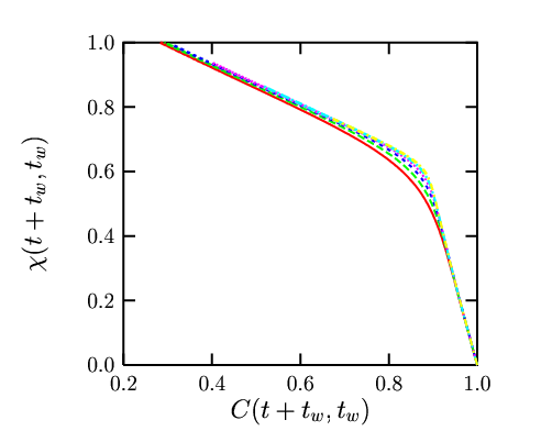

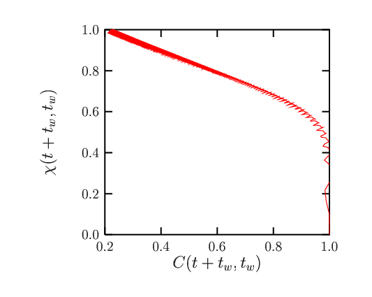

13.8 Systems of finite size: preasymptotic behavior
The previous discussion shows that the correlation scales (time-scales) play a very important role in the global behavior of the systems. For relaxational systems we argued that the asymptotic parametric curve appears in the limit . The thermodynamic limit that is taken first ensures that the equilibration time, , diverges and cannot be reached by the waiting-time. For a systems of finite size, , the equilibration time is a function of . In consequence, the limit curve has a lifetime that is bounded by . When the waiting-time becomes of the same order of magnitude as , the curve starts changing to approach the equilibrium asymptote, the straight line of slope . The way in which the approach to equilibrium is achieved is not known in general. It is a very difficult problem even for fully-connected models and there is little hope to solve a problem in sufficient detail as to be able to determine all the crossovers. This might be possible for the model of ferromagnetic growth or for the spherical sk disordered model. Crisanti and Ritort [160] analysed the crossover to equilibrium in the spin model with numerical simulations.
13.9 Critical dynamics
Godrèche and Luck studied the coarsening dynamics of ferromagnetic models quenched to the critical point . Spatial correlations develop in the system but only up to a length scale that grows as with the dynamic critical exponent. The equilibrium magnetization, , and, hence, , vanish. Still, the dynamics is highly non-trivial. For finite though long a stationary regime for and an interrupted aging regime for can be identified even if they are not clearly separated by a plateau in the correlation at a finite . In the former regime, the correlation and response are stationary and satisfy fdt. In the latter
| (13.5) |
with and the usual static critical exponents and and two scaling functions. As increases the stationary regime arrives up to lower values of and when grows to infinity the full decay is stationary as in equilibrium. Since the interrupted aging part of and decay only algebraically with the plot for finite though long is very rich with a non-trivial functional form. Similar results were obtained for the critical dynamics of the XY model [124].
13.10 Connection with equilibrium
The relation
| (13.6) |
between the static and non-equilibrium dynamic properties of slowly decaying systems, where is the non-equilibrium relation between integrated response and correlation function as defined in Eq. (11.5.3) and is the probability distribution of overlaps 11 1 The overlaps are given by the correlation between two equilibrated configurations. in the perturbed Gibbs state, became apparent from the analytic solution to some mean-field models.
This relation holds in the exact solution to the sk model [104] and the problem of a finite dimensional manifold embedded in an infinite dimensional space in the presence of a random potential with long-range correlations [96, 36]. It is not verified in the exact solution to the spin model and the manifold in a random potential with short range correlations. The reason for this discrepancy is that for the latter models the dynamics in the limit approaches the threshold and not equilibrium. More precisely, all generalized susceptibilities, and in particular the energy density, approach a limit . In all cases the dynamics occurs in a region of phase space that is different from the one sampled in equilibrium and, for spin models and the like it has different statistical properties. For the former models, even if still the region of phase space explored by the dynamics is different from the one corresponding to the equilibrium states, its statistical properties can be thought to be somehow equivalent, since , and the relation (13.6) holds.
More recently, Franz, Mézard, Parisi and Peliti proposed that the connection (13.6) goes beyond mean-field and applies to finite systems in which all dynamic susceptibilities converge to their equilibrium values, linking in this way the (easy to measure) non-equilibrium dynamics properties of realistic models to the (hard to measure) equilibrium properties of the same models. Since a threshold level as the one found for the spin model cannot subsist for ever in finite , they argued that the validity of Eq. (13.6) should be rather generic.
Several comments are in order. Corberi et al showed that there is a non-trivial nonequilibrium dynamic that does not satisfy Eq. (13.6) in one dimensional coarsening systems where the interface response does not vanish asymptotically (see Section 13.1). Even if the hypothesis of convergence of the generalized susceptibilities is not verified in this model, it provides a very simple example where the relation (13.6) does not hold. It might be possible to extend this result to domain growth in with an interface geometry such that the domain wall response does not vanish asymptotically. This problem deserves further study.
Based on numerical simulations, Marinari et al claimed [125] that the relation (13.6) is verified in the ea. As pointed out by Berthier, Holdsworth and Sellitto in the context of the xy model [124] and by A. Barrat and Berthier [113] in the context of the and ea models, one has to be extremely careful when extrapolating the numerical results obtained for finite waiting-time out of equilibrium and finite size in equilibrium. Indeed, these authors showed that one can tune the finite waiting-time and the finite size to have a relation like (13.6) well before the asymptotic limits are reached and even in the trivial phase of the xy and ea models.
Finally, it is worth stressing that a non-trivial has been found in explicitly out of equilibrium situations for which equilibrium is trivial as, for instance, in rheological measurements of super-cooled liquids or in the long-time dynamics of super-cooled liquids before equilibration is reached. Indeed, non-trivial curves have been found in glassy model above the putative in Lennard-Jones systems and at finite in models for which like the kinetically constrained lattice models [53, 54].
In conclusion, a better determination of which are the conditions under which (13.6) holds is necessary.
14 Effective temperatures
Temperature has remained an ill-defined concept until the development of thermodynamics and statistical mechanics. Evidently, the fact that a quantity, called temperature, must characterize the sensation of coldness or warmth has been known since the old times. However, temperature was usually confused with heat.
The thermodynamics is an empirical theory based on four postulates that has been developed to determine some properties of the macroscopic objects without knowing the details of their constituents and interactions. After , an isolated and finite system reaches an equilibrium macroscopic state that can be characterized by a small number of parameters, the state variables. Temperature is one of these parameters. The first law states that energy is conserved in an isolated system after having established the equivalence between heat and work. The zeroth law states that if two systems are in thermal equilibrium with a third, then they are also in equilibrium between them. The temperature is determined by an auxiliary measurement. One sets a thermometer in contact with the system, waits until thermal equilibrium is established and then determines the temperature by calibrating the reading of the thermometer. If one repeats this procedure with a second system, equilibrated with the first one, the first law ensures that the thermometer will itself be in equilibrium with the second system and, consequently, its reading will yield the same temperature. Hence, all systems in thermal equilibrium among them are at the same temperature.
The statistical mechanics establishes a bridge between the mechanical description of the microscopic constituents of the system and its macroscopic behavior. It yields a precise sense to the concept of temperature. To illustrate this statement, let us take an isolated system in the microcanical ensemble with volume and internal energy . The entropy of the system is defined as with the number of accessible states with mean energy between and . The microcanonical definition of temperature is given by , evaluated at . The development of statistical mechanics allows one to show that this definition is equivalent to the thermodynamic one. One can equally find it with the canonical and grandcanonical formalisms.
The previous paragraphs describe the behavior of systems in thermal equilibrium. What can one say about the systems that evolve out of equibrium? Can one define a temperature for them? Or is it at least possible for a subclass of nonequilibrium systems? If this holds true, can one use this definition as a first step towards the development of a thermodynamics and a statistical mechanics for systems far from equilibrium?
Hohenberg and Shraiman discussed the possibility of defining a temperature for certain systems out of equilibrium [126] using the modification of fdr. In Ref. [112] we critically studied the definition of such an effective temperature, , we insisted on the need to reach a regime with slow dynamics (related to small entropy production) to be able to define such a “state variable” and we demonstrated the importance of analyzing it in separated time-scales. In this Section we show in which sense the expected properties of a temperature are satisfied by and we display some numerical tests.
14.1 Thermodynamical tests
14.1.1 How to measure a temperature
In normal conditions, the temperature of an object is measured by coupling it to a thermometer during a sufficiently long time interval such that all heat exchanges between thermometer and system take place and the whole system equilibrates.

Let us call the instant when thermometer and system are set in contact. For simplicity, we choose to describe the thermometer with a single variable . In order to have a statistical measure of the object’s temperature [127, 72] we couple the thermometer to independent copies of the system. Each system is characterized by a variable , . The energy of the total system is
with the potential energy of the isolated thermometer and the one of the th isolated system. Note the similarity between this coupled model and the treatment of system+environment done in Section 4 and the discussion on the harmonic oscillator coupled to a complex bath in Section 7.4.4. For a given value of , the last term acts as an infinitesimal field that is coupled to the observable of each copy. The equation of motion of the thermometer reads
| (14.1) |
Again for simplicity we choose an observable with vanishing mean where the angular brackets represent the average over different histories of the system (see Section 5.1) or the average over different systems, i.e. . When the averaged observable does not vanish we use the difference between the observable and its average as the fundamental quantity. The index indicates that the average is taken in the absence of the thermometer. We denote the averaged in the presence of the thermometer. Equation (14.1) can be rewritten as
| (14.2) |
with the linear response of the observable to the change in energy performed at time . The force is a sum of independent random variables and due to the central limit theorem, it becomes a Gaussian variable with vanishing average and variance
| (14.3) |
for large at first order in . Thus, the evolution of the thermometer is determined by a Langevin-like equation [cfr. Eq. (4.7)] with a correlated noise and a retarded friction generated by the coupling to the systems. For a generic system out of equilibrium there is no relation between and . For the problems we are interested in there is one. Next we explore the consequences of the modification of fdt for the reading of the thermometer.
If the systems are equilibrated with their environments fdt holds and it ensures that is related to by , with the temperature of the thermal bath. The thermometer is then coupled to an equilibrated colored bath and it will eventually reach equilibrium with it. The reading of the thermometer is defined from the value of its asymptotic internal energy and it has to be callibrated from the characteristics of the thermometer that, of course, must be known before starting the measurement. If one takes a simple harmonic oscillator as a thermometer, one proves that the internal energy approaches . This is the result expected from equipartition since the oscillator has only two degrees of freedom (position and momentum).
Imagine now that the systems are glassy of the type discussed in Section 12. If one studies a system with two correlation scales such that
with the temperature of the thermal bath and a different value read from the modified fdt relation. The reading of the thermometer, or its asymptotic internal energy density, is found to be [112]
| (14.5) |
where is the characteristic frequency of the thermometer, is the Fourier transform of the correlation function with respect to the time-difference and is the out of phase susceptibility defined in Eq. (5.8).
If the characteristic frequency is very high, the thermometer evaluates the evolution during the first step of the relaxation , one finds and one identifies with the temperature of the system. Instead, if the characteristic frequency is very low, the thermometer examines the behavior of the system in the long time scales, in the example, one finds and one identifies as the temperature of the system.
One can easily generalize this discussion to a problem with many correlation scales, each with a different value of the effective temperature. In order to measure them it is sufficient to tune the characteristic frequency of the oscillator to the desired scale.


A concrete realization of this measurement corresponds to a generalization of the Brownian motion experience of Perrin in which one follows the evolution of a tracer immersed in the fluid. If the latter is equilibrated at temperature , after a short equilibration period, each component of the averaged kinetic energy of the tracer approaches . Instead, if the fluid evolves out of equilibrium, one can choose the mass of the particle (that plays the role of the characteristic frequency in the previous discussion) in order to examine the rapid dynamics, or the slow dynamics. The tracer acquires an averaged kinetic energy with the value of the effective temperature in the time scale explored. Berthier and J-L Barrat [121] performed this measurement in a numerical experiment using a dense liquid modeled as in Eq. (2.4) under homogeneous shearing in contact with a thermal bath at temperature as a fluid. They chose a Lennard-Jones particle as a tracer with mass . The left panel shows the asymptotic value of the transverse component of the averaged kinetic energy (transverse to the shearing rate direction) as a function of the mass of the tracer. One clearly sees how the effective temperature interpolates between the value at small masses and the value for large masses. The trend can be easily understood. A very light tracer easily reacts to the quick bombardment of the particles in the fluid and it feels the temperature of the bath via the rapid scale of relaxation. A heavy tracer instead can only move via large rearrangements of the fluid and these correspond to the slow part of the relaxation. The transition between the two values is very smooth and it occurs over several orders of magnitude in the mass. The consistency of the explanation, i.e. the relation between and the fdt relation, will become explicit in Section 14.1.2.
14.1.2 Zeroth law
A temperature, even if it is defined out of equilibrium, should control the direction of heat flows and the partial equilibration between observables in interaction. (Two observables interact if and only if the crossed linear response , as defined in Eq. (5.5), does not vanish.)
With a pair of observables and one constructs two self and two cross correlations and responses. In each correlation scale the fdt relation is modified by a constant factor with which one constructs the effective temperature. If the notion of an effective temperature is correct, two interacting observables that evolve in the same time-scale should acquire the same value of . The equilibration between different observables is well defined only in the limit of small heat, or energy, exchanges. This limit is achieved in a free relaxing system when the waiting time becomes very long or in a driven system rendered stationary when the nonconservative force vanishes. It is only possible for observables evolving in the same time-scale (note that even a single observable can have several values of the effective temperature when examined on different time-scales). We call partial equilibrations those arriving in the same time-scale. In contrast, if the two observables and do not interact they should evolve in different time-scales.
The property of partial equilibration has been proven analytically for the fully connected models solved in Section 12 [112] and, later, for all perturbative approximation of more realistic models under the assumption of there being a slow dynamics with a sharp separation of time-scales [72, 130]. It can be seen numerically as follows. Take, e.g., two spin models with different exchange strengths, and in contact with the same thermal bath at temperature and couple them linearly with a term where and are the dynamic variables of each system and is the coupling constant. (Other couplings are, of course, possible.) When the two systems evolve independently and their ’s in the aging scale take different values. If we now let the coupled system ) evolve it will reach an asymptotic limit (roughly when the energy of the full system decays very slowly). In this limit we trace the fdt parametric plots for the two self and cross and ’s. We observe that if the cross responses vanish and the effective temperatures still take different values in the aging scales that are now forced to evolve with different scalings. Instead, if , the cross responses do not vanish, the two systems lock and in the aging scale acquires the same value for both self and cross fd relations. Note that for the manifold, all modes have the same value of the effective temperature in the same correlation scale. This is achieved internally and it means that all modes are in interaction.
Partial equilibrations have been tested numerically by Berthier and J-L Barrat [121] in the dense homogeneously sheared liquid discussed in Section 14.1.1 (partial equilibrations simply relaxation Lennard-Jones mixture were studied by Kob and J-L Barrat in [58]). The relevant correlators for this system are the wave vector dependent incoherent scattering functions and their associated responses. Berthier and Barrat measured these two-time functions for the same and different species and several values of the wave vector. Figure 20 shows the parametric fdt plots. All the curves have a broken line form with a first part with slope and a second part with a common slope . The value is identical to the result found monitoring the kinetic energy of the tracer (see Section 14.1.1) demonstrating that the scenario is consistent. Note that in this case we cannot tune the coupling between different wave vectors as we did when we externally coupled the two spin model. The fact that in the slow scale is the same for all wave vectors studied shows that they interact. This is also seen from the fact that the cross responses do not vanish. Coupled oscillator models with parallel or sequential Montecarlo dynamics do and do not partially equilibrate, respectively. [129]. In the latter case the thermal conductivity is very small and one is in situation in which, effectively, .
Intriguingly, the fact that each time-scale has its own effective temperature has been shown to fail in two models. These are the trap model [48] and the Ising chain at [48, 119, 120] when special perturbations are applied. In both cases one can construct observables that evolve in the same time-scale but have different values of the effective temperatures. In the first case, the failure might be adscribed to the fact that the model does not have an equilibrium state. This is not the case in the second model though. The origin of the failure might then be related to having used special observables, see the discussion in [48]. Still another pathology was already signaled for this problem: the global correlation and response decay in a single time-scale but the asymptotic is a curve contradicting the notion of a correlation-scale dependent effective temperature. It is quite plausible that this problem is also related to the failure of the relation between dynamics and statics discussed in Section 13.10. A good understanding of the conditions under which this property holds is still lacking. Experiments in laponite show some mismatch between the value of found with mechanical and electrical measurements. The reason for this is unclear [61].
One can also verify that the heat exchanges go from the higher values of to lower ones. However, it is still not clear why one can have a partial equilibration to a higher value of than those of the two independent observables, as it has been obtained analytically for some solvable fully-connected models.
14.1.3 Auxiliary thermal baths
A supplementary verification of the thermodynamic character of the effective temperature comes from the study of the action of complex thermal baths on the dynamics of simple systems, as discussed in Section 14.1.3, or glassy systems.
We found that an arbitrarily weak auxiliary bath with small has an important effect provided it is sufficiently slow and its temperature is within the range of values of the effective temperatures of the slow dynamics. The (slow) time dependence of all and ’s are affected by a time rescaling . This is such that the time-scale which has an effective temperature equal to the temperature of the auxiliary bath, say , is locked to the time-scale of the bath. In particular, if we couple an aging system with a bi-valued to a composite stationary bath with two time scales, and and two temperatures and , respectively, we find that the system becomes stationary if , and is hardly affected if . More generally, an aging system with multiple effective temperatures, , becomes partially stationary for all the time-scales with , but still ages for time-scales with . We found this behavior in Montecarlo simulations of the ea model [130].
14.2 Temperature fixing by susy breaking
For any model one can derive a set of integro-differential equations that couple all two-point functions. These admit a representation in terms of the super-correlator . In the asymptotic limit in which we neglect the time-derivatives, these equations are invariant under any change of supercoordinates, , that have unit superjacobian [162]. Fixing the time-reparametrisation (the function in each correlation scale) and the value of the effective temperature corresponds to breaking this large symmetry group to a subgroup [130].
14.3 Fictive temperatures
“Fictive temperatures” are phenomenological concepts that have been used to describe experimental data [131] (see also [132]). The basic idea has been to claim that, when crossing , the system remembers its equilibrium configuration before the quench and it remains effectively at a higher temperature . Several refined prescriptions to extract time and preparation dependences of have been proposed. The relation between and has been discussed in [112]. Here we simply stress that even if the same basic idea can be used to interpret , the latter has the properties of a thermodynamic temperature while this is not obvious for .
14.4 Nonequilibrium thermodynamics
Once equipped with a bonafide effective temperature the natural next step is to try to construct a thermodynamics for such systems out of equilibrium. This has been proposed by Nieuwenhuizen [133] based on two previous results: (1) similar constructions done using the fictive temperatures by Tool, Moynihan and others [131]. (2) the relation between the dynamics and the tap approach that we shall discuss in Section 15. The idea is to define generalized thermodynamic potentials in which intervenes as a supplementary parameter (one can also include other state variables as an effective pressure, etc.). For the fully connected models these potentials have a precise meaning based on the tap analysis (Section 15). Their validity for more realistic models is still an open problem.
14.5 Statistical mechanics
Edwards measure
In the 80s Edwards proposed that the stationary properties of dense granular matter under a weak forcing can be determined with a flat distribution of the blocked configurations, i.e. those in which no grain is able to move) at the chosen density [134]. Note that this is possible in granular matter since the external temperature is irrelevant. Following this “microcanonical” approach the logarithm of the number of blocked configurations at constant density defines an entropy from which one obtains a compactivity by simple derivation with respect to the density. Extending this prescription one can define an Edwards’ temperature for soft systems by considering blocked configurations at fixed energy and computing .
Edwards’ temperature can be calculated explicitly for the fully connected models at zero external temperature (again using techniques discussed in Section 15). Surprisingly, one finds that its actual value coincides with the value taken by defined from the modification of fdt in a purely dynamic calculation. This result has boosted the study of solvable models in low dimensionalities analytically and more realistic systems numerically to check if the coincidence goes beyond the fully-connected case. Until now, several models where Edwards’ distribution yield very good results have been exhibited [122, 135] while some others where it fails have also been shown (e.g. the random field Ising model [122]). In the latter cases one finds a well-defined while Edwards’ measure fails to give the correct results. The result of including additional constraints on the configurations counted have also been analysed and naturally improve the results derived from Edwards’ measure. This area of research is very active and more work is necessary to determine the limits of validity of Edwards’ proposal.
The definition of Edwards’ measure is unambiguous since it is a zero temperature entity based on the study of minima of the potential energy. An extension to finite necessitates the analysis of a free-energy landscape. This can be done analytically for fully-connected models as explained in Section 15. In finite cases for which one is forced to use numerical techniques it is not, however, obvious how to define, let alone compute, the entropy .
Inherent structures
The inherent structure approach of Stillinger and Weber [136] has been recently revisited and extended to study dynamic properties of glass formers and glasses [137]. The original approach, even if static, is close to the ideas of Edwards. At the static level it consists in dividing the partition function in inherent structures, or pockets of configurations around minima of the potential energy, and transforming the sum into sums over minima and the configurations associated to them. In order to connect with the dynamics, one computes the entropy of the inherent structures and then derives an inherent structure temperature with a similar prescription to the one of Edwards. The sampling of the inherent structures numerically is a non-trivial issue.
A critical analysis of the applicability of this approach at finite temperatures has been presented by Biroli and Monasson [142] who stressed the need of analyzing the free-energy, instead of the potential energy, at finite . They also compared with the tap analysis discussed in Section 15. Having said this, the use of the inherent structure approach has been rather successful when confronted to [137].
15 Metastable states
The aim of the tap approach is to define and study a free-energy density as a function of the relevant order parameters [56]. Its stationary points are the (stable and unstable) metastable states. For a fully connected Ising magnet the tap free-energy density simply depends on the averaged global magnetization and, below , has the form drawn on the right panel of Fig. 1. The vanishing global magnetization is not a good order parameter for disordered spin systems and one is forced to introduce all local ones. The approach can be extended to describe classical and quantum systems in and out of equilibrium [143, 144]. Under different names similar approaches appear in other branches of condensed matter physics. The density functional theory of the inhomogeneous electron gas in solids or the dynamic mean-field theory of strongly correlated electrons are very similar in spirit to the tap approach [91].
The clearest way of deriving the tap free-energy density for disordered models is based on two ingredients: one identifies an adequate perturbative expansion, and one Legendre transforms the standard free-energy density with respect to a well-chosen set of parameters. When these two choices are correctly done, only a finite number of terms in the expansion do not vanish for typical configurations of disorder for infinite dimensional models. In finite one can attempt a large expansion [146].
For spin-glasses at low- the tap free-energy density has an infinite number of stationary points. The tap approach gives us access to the complete organization of metastable states of any type of stability (minima, saddles of all types, maxima). In particular, this has been analysed in great detail for the spin model and the like since we expect it to mimic what occurs in real glassy systems though in an exaggerated manner.
In the following we first derive the tap free-energy density for a generic spin model with Ising or spherical variables. Next we summarize the consequences of this approach for the spin spherical model. We also briefly explain how the number of metastable states is computed and how this depends on the parameters in the model. We explain how the approach is generalized to deal with dynamic properties. This full set of results gives us a complementary view of the non-equilibrium dynamics and serves as the basis for an image of the dynamics of finite glassy models.
15.1 Equilibrium
Before describing the tap approach let us summarize the equilibrium behavior of the mean-field models as derived from the analysis of its disordered averaged free-energy density with the replica trick. Again the three classes, ferromagnetic-like (), glassy-like ( [167] and spins-glass-like (sk) [9] models have different characteristics.
For the spherical spin model with [167] the standard Parisi Ansatz [69] yields a static transition at from a paramagnetic phase where a replica symmetric Ansatz solves the problem to a glassy phase where a one step replica symmetry breaking Ansatz is needed. At low ’s, the breaking point parameter, , and the Edwards-Anderson order parameter, , in the Parisi matrix are fixed by requiring that the free-energy density be a maximum. This yields a static transition temperature, , given by the set of equations and . One can check that . The static transition is discontinuous in the sense that jumps at but it is of second order thermodynamically since all susceptibilities are continuous across . The equilibrium energy density at is given by the implicit equation . One checks that
A modified prescription to determine the breaking point, , in the one step Ansatz yields different results. If instead of extremizing with respect to one requires that the solution be marginally stable by setting the replicon eigenvalue of the matrix of quadratic fluctuations [175] to zero, leads to a different solution with a dynamic meaning. (All other eigenvalues are positive.) Namely, one finds a transition from the paramagnetic to the glassy phase at a higher temperature that coincides with the dynamic critical temperature found with a purely dynamic calculation, . Moreover, coincides with the dynamic one and the breaking point yields the ratio . Consequently, all one-time quantities as the asymptotic energy density and generalized susceptibilities coincide with the ones found dynamically (e.g. ). The fact that with the condition of marginal stability we access the region of phase space reached dynamically is due to thte fact that with both we search for the path of flat direction formed by the threshold level, as explained below.
When instead [108], the replica solution below is replica symmetric with a non-vanishing and marginally stable. The static transition is continuous, dynamic and static transition temperatures coïncide, , and [109]. The gap between the threshold and the equilibrium level collapses and the static energy density is the value reached dynamically, . Still the nonequilibrium dynamics does not stop in finite times with respect to .
For sk the equilibrium calculation needs a full replica symmetry breaking solution [9]. This can be interpreted as being equivalent to having a sequence of correlation scales in the nonequilibrium dynamics. The static transition is continuous, the static and dynamics are identical, the relation in (13.6) holds and all one-time quantities coincide with the equilibrium values. The static solution is also marginally stable.
From these three paragraphs one observes that the structure of the static and dynamic solution of purely potential mean-field problems is indeed very similar. One can propose a “dictionary”
| rs | ||||
| 1 step rsb | ||||
| full rsb |
while remembering that the replica solution that describes the statistical properties of the region of phase space reached dynamically has to be determined using the condition of marginally stability – and not equilibrium. This connection between replicas and dynamics has been extensively exploited to use the replica trick as a substitute for dynamics. In fact, partial information about dynamics as the dynamic critical temperature, the value of , etc. is thus obtained. One has to keep in mind though that many aspects of the dynamics go beyond static calculations. Features like the existence of an effective temperature have been shown in models with trivial statics [53, 54] or above the dynamic transition when non-potential or time-dependent forces are included [19, 26].
15.2 Static tap approach
In the introduction to this Section we announced that two choices facilitate the derivation of the tap free-energy density. In order to use a good perturbative expansion we weight a part of the original Hamiltonian with a parameter . For the spin model we simply propose
| (15.6) |
In other models we weight the higher order interactions with without modifying the quadratic terms. The idea is to expand in powers of and set at the end of the calculations to recover the original model [145, 146].
The second important step in the derivation is the choice of the order parameters to use in the Legendre transform of the free-energy density. For spin models these are the averaged local magnetizations and a global spin constraint . The Legendre transform reads
| (15.7) |
The trace represents a sum over all configurations of the spins, e.g. for Ising and for spherical variables. Requiring stationarity with respect to the Langrange multipliers and one obtains
| (15.8) |
for all values of . The angular brackets indicate the statistical average over the spins using the full Botzmann weight in (15.7). Since the rhss depend on and these equations can be inverted to yield and . that one substitutes in (15.7) to write as a function of . Henceforth we drop the parameter dependence and simply note . The introduction of the parameter allows us to express as a power series in :
| (15.9) |
For the spin model and the like this is equivalent to a high expansion. In other cases it is an expansion around an “equivalent” free theory. Interestingly enough only a finite number of terms contribute to the series for fully connected models. For finite dimensional cases a truncated series yields an approximation around mean-field.
The zero-th order term depends on the nature of the spins considered:
These are the entropies of independent Ising or spherical spins constrained to have local magnetizations . The first order term is proportional to
| (15.10) |
In the first equality, the last two terms on the rhs vanish due to Eqs. (15.8). The average in the first term factorizes since it has to be taken with the free-action (). The quadratic term in the expansion is proportional to
| (15.11) |
with . This term has been computed using the following identities. First, the variation of in Eq. (15.7) with respect to and yields and . Taking the variation with respect to and evaluating at one has
| (15.12) |
Now, the contributions are proportional to and these can be estimated by replacing its value by since . As done for the first order term we factorize the thermal averages evaluated at and
| (15.13) | |||||
| (15.14) |
where we introduced the overlap or (static) Edwards-Anderson parameter,
| (15.15) |
Higher order terms in the series expansion are sub-leading in and do not contribute in the thermodynamic limit. Thus, for these mean-field models the tap free-energy density is made of three terms: the zero-th order has an entropic origin, the first order is the interaction term in the mean-field approximation which is exact for fully connected models, and the second order is the reaction or Onsager term.
15.3 The tap equations
The variation of the tap free-energy density, , with respect to (and for the spherical model) yields the tap equations. For the spherical model one finds [147]
| (15.16) | |||
| (15.17) |
The study of these equations is simplified by defining the angular variables that verify the spherical constraint . Multiplying Eqs. (15.16) by and summing over we rewrite them in terms of the zero-temperature energy density :
| (15.18) |
The overlap is related to by
| (15.19) |
Equation (15.18) does not depend on while (15.19) does. The multiplicity of solutions at a given is entirely determined by Eq. (15.18), see Section 15.5. The existence or not of these solutions has to be tested with Eq. (15.19). The remaining Eq. (15.17) fixes .
Conveniently rewritten Eq. (15.19) is quadratic and yields
| (15.20) |
This equation admits a real solution only if , the threshold energy density at . The minus (plus) sign correspond to a minimum (maximum) of the free-energy. The physical is then associate to the minus sign. With this choice, takes its maximum value on the theshold and then monotonically decreases until reaching its minimum value on the equilibrium level, .
For fixed and the lhs in Eq. (15.20) has a bell shape form. When , and is finite. The maximum is located at and it has a height . Each solution at that corresponds to a given can be followed to finite until it disappears at when the lhs reaches the maximum. One can check that the tap solutions do not merge nor bifurcate as a function of . Then at any temperature we label the tap solutions with their associated zero temperature energy density .
Plugging in Eq. (15.19) we find that the overlap is given by the equation
| (15.21) |
The threshold energy density and the overlap coincide with the asymptotic value of the dynamic energy density and the Edwards-Anderson parameter at , respectively. Thus, the nonequilibrium dynamics approaches asymptotically the threshold level.
15.4 Stability of, and barriers between, the tap solutions
The spectrum of the free-energy Hessian around a stationary point of the tap free-energy is a shifted semi-circle. The lowest eigenvalue is greater than zero for sub-threshold free-energy densities (or zero-temperature energy density). This means that for typical stationary states are minima. Instead, near the threshold drops to zero as [12]
| (15.22) |
and the stationary states on the threshold are typically marginal in the sense that they have many flat directions.
Even if the connection between dynamics and the static tap free-energy landscape is not obvious a priori, it has been proposed and used in several works [11, 12]. The formalism in Section 15.8 and [148] settles it on a firm ground. If one imagines that the dynamics can be viewed as the displacement of a representative point in the free-energy landscape, not only the organization minima, saddles and maxima has to be known but also how do the barriers between these stationary points scale with . Few results about barriers exist and, in short, they are the following. The barriers between threshold states vanish when [3, 149] and there is no sharp separation between them. This has been proven by analyzing the constrained complexity, related to the number of threshold states that have an overlap with a chosen one ( where and are the two configurations). This complexity decreases with increasing values of and it vanishes as a power law at . This means that one can find threshold states that are as similar as required to the chosen one. The threshold level is then a series of flat connected channels. The non-equilibrium dynamics starting from random (typical) initial conditions approaches this level asymptotically and it never stops since the system drifts in a slower and slower manner as time evolves following these flat directions [12]. On the other hand, the barriers between equilibrium and metastable states have been estimated to be [147, 149]. One can guess that the barriers between sub-threshold tap states also scale with . For finite the dynamics should penetrate below the threshold and proceed by thermal activation. An Arrhenius-like time will then be needed to descend from one level to the next. Naturally one should see another kind of separation of time-scales develop. Simulations of the spin model for finite confirm the existence of metastable states below the threshold. This is most clearly seen following the evolution of the energy density of the model weakly perturbed with a non-potential force. One sees periods of trapping in which the energy-density is fixed to a given value and periods in which the system escapes the confining state and surfs above the threshold until being trapped in a new state [18, 26, 19] (see also [160] a numerical study of the finite -spin model).
15.5 Index dependent complexity
At low ’s the number of stationary points is exponential in . This suggests to define the complexity :
| (15.23) |
where is the number of solutions with energy density . Actually, one can refine the study by grouping the stationary points of the tap free-energy density into classes according to the number of unstable directions. Thus, minima are saddles of index , saddles with a single unstable direction have index and so on and so forth. The complexity of each kind of saddle is , where denotes the index of the considered saddles. For the spherical spin model, their average over disorder, , are ordered in such a way that [150]
Thus, when minima are exponentially dominant in number with respect to all other saddle points. Moreover, one proves that the complexities vanish at a -dependent value of . The complexity of minima is the last one to disappear at .
15.6 Weighted sums over tap solutions
The thermodynamics at different is determined by the partition function, . De Dominicis and Young [151] showed that the equilibrium results obtained with the replica trick or the cavity method are recovered from the tap approach when one writes as a weighted sum over the tap stationary states.
Indeed, if one divides phase space into pockets of configurations that surround the stationary points of the tap free-energy one can carry out the statistical sum on each sector of phase space:
| (15.26) |
where the index labels the tap solutions and represents a restricted sum over the configurations that belong to the pocket associated to the solution . In order to make this separation precise one needs to assume that the barriers separating the pockets diverge in such a way to avoid ambiguities when associating a configuration to a tap solution. The restricted sum is related to the free-energy of the tap solution and the partition function becomes . Thus, any statistical average can be computed using the weight . The sum over solutions can be replaced by an integral over free-energies if one introduces their degeneracy and their associated complexity, , with ,
| (15.27) |
The complexity is a self-averaging quantity, we then write . When the integral is dominated by the solutions that minimize the generalized free-energy, . This is achieved either by with or by states that do not have the minimum free-energy if their complexity is finite, in which case [138]
| (15.28) |
Minima of the generalized free-energy density with higher () or lower () free-energy density are metastable.
Above the dynamic transition
The paramagnetic or liquid solutions , , dominate the partition sum, . States with exist in this range of temperatures but they do not dominate the sum.
Between the static and dynamic transitions
The paramagnetic state is fractured into an exponential in number of non-trivial tap solutions with . Their free-energy density and the partition sum are given by Eq. (15.28). Each of these states has a rather high free-energy that is counterbalanced by the entropic contribution. Besides the states that dominate the partition sum, a very large number of other metastable states, with higher and lower free-energy density, also exist but are thermodynamically irrelevant. It turns out that coincides with the extrapolation of from to this temperature region even if the paramagnetic solution does not exist. Note that in this temperature regime the standard replica calculation fails since it tells us that the equilibrium state is the simple paramagnet. Refinements on this method are able to extract more precise information about the non-trivial states contributing to equilibrium [149].
Below the static transition .
An infinite though not exponential in number of states with the minimum free-energy density dominate the sum. The complexity vanishes and this is associated to an entropy crisis. This is similar to the argument used by Kauzmann to justify the existence of a dynamic crossover at since, otherwise, the projection of the difference between the liquid and the crystal entropy would vanish at . In this sense, this model realizes the Kauzmann paradox at .
15.7 Accessing metastable states with replicas
The replica trick can be improved to access the non-trivial metastable states existent between and [169, 138, 139] using a “pinning-field” or a “cloning method”. Let us sketch how the latter works. Consider copies or clones of the systems coupled by an attractive, infinitesimal (but extensive) interaction. The free energy for the system of clones reads:
| (15.29) |
using the formalism described in the previous Subsection. On the other hand, the free-energy density of the clones can also be computed with the replica approach:
| (15.30) |
where we used the fact that the free-energy density is self-averaging. Since the attractive coupling between the clones is infinitesimal, the computation of the rhs of Eq. (15.30) reduces to the calculation of , where the replica symmetry between the groups of -replicas () is explicitly broken. When the system is in the replica symmetric phase (), the problem becomes one where one has to study one-step replica symmetry breaking solutions non-optimized with respect to :
| (15.31) |
where is the free-energy-density computed by using replicas, is the Edwards-Anderson parameter and is the breakpoint or the size of the blocks in the replica matrix. (For simplicity we consider that the inter-state overlap equals zero [9].) Since the integral on the lhs of Eq. (15.31) is dominated by a saddle point contribution, one finds that, for a given , fixing the value of one selects the states with a given free-energy-density . The relationship between and reads
| (15.32) |
Note that within this framework one does not optimize with respect to . Instead, is a free parameter and, by changing the value of , one selects different groups of metastable states. Inversely, choosing a value of the free-energy density one determines an “effective temperature” . This value coincides, indeed, with the dynamic result for in the aging scale when . Otherwise, it gives a free-energy level dependent effective temperature. If one pursues the empirical relation between this parameter and the dynamic effective temperature this result means that when the system evolves in sufficiently long time-scales as to penetrate below the threshold it takes different values of depending on the deepness it reached.
Mézard and Parisi generalised this approach to search for a Kauzmann critical temperature () and characterise the thermodynamic properties of the glassy phase below in finite interacting particle systems. The mean-field nature of the approach has been stressed by Thalmann [141] who showed that there is no lower critical dimension.
15.8 Dynamics and quantum systems
The derivation of the tap equations presented in Section 15.2 can be generalized to treat other problems as the real-time dynamics [143] of the same models or their quantum extensions [144]. Again, the procedure can be made easy if one correctly chooses the perturbative expansion and the order parameters. To study the real-time dynamics of the classical problem one is forced to Legendre transform with respect to the time-dependent local magnetization, the two-time correlation and the response [143]. The presentation is further simplified when one uses the susy notation introduced in Section 8.2 that renders the dynamic formalism very close to the static one. For quantum problems in equilibrium one uses the Matsubara representation of the partition function and then Legendre transforms with respect to the imaginary-time correlation as well as the local magnetizations [144]. In order to derive tap equations for a quantum problem in real-time one should use the Schwinger-Keldysh formalism.
The derivation and study of dynamic tap equations justifies the interpretation of the asymptotic non-equilibrium dynamics in terms of the local properties of the tap free-energy density landscape. Biroli [143] showed that the dynamics in the tap free-energy landscape is in general non-Markovian due to the presence of memory terms in the dynamic tap equations. In the very long-time limit and for random initial conditions the contribution of these terms vanishes and one proves that the dynamics is a relaxation following flat directions in the tap free-energy landscape (the threshold) as proposed in [12, 3].
16 Conclusions
We discussed the behaviour of a family of disordered models that yield a mean-field description of the glass transition and dynamics of super-cooled liquids and glasses. The relevance of these models to describe structural glasses was signaled and explained by Kirkpatrick, Thirumalai and Wolynes in the 80s [11]. Their nonequilibrium dynamics and hence the connection with other systems far from equilibrium started to develop more recently [12].
In short, their behaviour is the following. The dynamic transition arises when the partition function starts being dominated by an exponentially large number of metastable states yielding a finite complexity. The static transition instead is due to an entropy crisis, i.e. it occurs when the complexity vanishes and the number of states is no longer exponential in , just as in the Adams-Gibbs-di Marzio scenario [177]. These transitions mimic, in a mean-field way, the crossover to the glassy phase at and the putative static transition at (or ) of fragile glasses, see Fig. 2-left [11].
The equilibrium dynamics close and above coincides with the one obtained with the mode-coupling approach [11]. It describes the relaxation of super-cooled liquids and it contains its most distinctive feature of having a two step decorrelation. The first step is ascribed to the motion of particles within the cages made by their neighbours while the second one is the structural relaxation related to the destruction of the cages.
Below the equilibration time diverges with the size of the system and the models do not equilibrate any longer with their environments (unless one considers times that grow with the size of the system) [12]. This is very similar to the situation encountered in real systems below . The experimental time-window is restricted and one is not able to equilibrate the samples any longer below . Aging effects as shown in Fig. 7 are captured. The correlations still decay to zero but they do in a waiting-time dependent manner. Their decay also occurs in two steps separated by a temperature-dependent plateau at a value related to the size of the cages. One can interpret their stiffness as increasing with the age of the system given that the beginning of the structural relaxation is delayed and slowed down for longer waiting-times.
The nonequilibrium dynamics below approaches a threshold level of flat directions in phase space and it never goes below this level in finite times with respect to the size of the system [12]. The aging dynamics corresponds to the slow drift of the point representing the system in the slightly tilted set of channels that form the threshold. The motion that is transverse to the channels is related to thermal fluctuations and the first stationary step of the relaxation towards , that charcaterises then the transverse “size” of the channel. The longitudinal motion along the channels is related to the structural relaxation. The tilt is proportional to the magnitude of the time-derivatives and these become less and less important as time passes. In more generalitiy one interprets the long but finite time nonequilibrium dynamics following saddles that are the borders between basins of attraction of more stable states in phase space [3].
For times that scale with the size of the system, , the sharp dynamic transition is avoided, the system penetrates below the threshold via activation and it approaches equilibrium in much longer time-scales. Metastable states below the threshold are typically minima [147, 150] (the fact that they are local minima can be checked studying the dynamics with initial conditions set to be in one of them [157, 139, 18]). This structure allows one to describe the cooling rate effects described in Fig. 2-right. For large but finite and sufficiently slow cooling rate, the system penetrates below the threshold via activation when this is facilitated by , i.e. when passing near . To which level it manages to arrive (roughly speaking to which of the curves in the figure) depends on how long it stays close to . The slower the cooling rate the lower level the system reaches with the ideal “equilibrium” glass corresponding to an infinitely slow cooling [158].
The region of phase space reached asymptotically in the thermodynamic limit is the threshold of flat directions. The replica analysis of the partition function gives an alternative way of determining its statistical porperties. Indeed, by evaluating the partition function on a marginally stable saddle-point in replica space one selects the threshold “states”. Dynamic information such as the value of is thus obtained with a pseudo-static calculation. Other facts as, for instance, the scaling of the correlation are not accessible in this way.
One of the hallmarks of the glassy nonequilibrium dynamics is the modification of the relation between correlations and responses, namely, the fluctuation-dissipation theorem. In mean-field models for structural glasses one finds that the integrated linear response is in linear relation with the associated correlation with a proportionality constant that takes the equilibrium value when the correlation is above the plateau and it takes a different value when it goes below the plateau [12]. This behaviour has been found in a number of finite dimensional glassy models numerically [58, 53, 54, 55].
The behavior just described corresponds to a family of mean-field disordered models to which the spin models with and the Potts glass belong. Other two families exist and they are related to ferromagnetic domain growth and spin-glasses. Two representative models are the spherical spin model with and the sk model, respectively. They are characterised by different scalings of the correlations in the aging regime and by different forms of the modification of fdt. The classification in families according to the nonequilibrium behaviour has a static counterpart given by the structure of replica symmetry breaking in the low- phase, see Section 15.1.
The modification of fdt allows one to define an observable and correlation-scale dependent effective temperature [112]. Fast observables like the kinetic energy are equilibrated with the environment and the effective temperature equals the thermal bath temperature for them. Other observables though show different values of the effective temperature depending on the time-scales on which one investigates them. The effective temperature has a thermodynamical meaning even if defined out of equilibrium. In particular, it can be directly read with a thermometer coupled to the desired observable and a zero-th law holds for interacting observables that evolve in the same time-scale. As one should have expected the effective temperature shares some of the qualitative features of the phenomenological fictive temperatures [131]. For instance, a system that is quenched from high temperatures has effective temperatures that take higher values than the temperature of the bath, etc. At the mean-field level, when , it is history independent but one expects it to depend on the preparation of the sample for finite size and finite dimensional systems. (This is in close relation to the discussion above on cooling rate effects.) There is still no precise determination of which are the necessary conditions a nonequilibrium system has to fulfill to ensure the existence of well-behaved effective temperatures. A clear condition are the need to reach a dynamic regime in which the dynamics is slow and heat exchanges are weak.
Once the effective temperature has been identified one interprets the behaviour in the low phase as follows: the system adjusts to a situation in which each observable sees two baths, one is the white external one and the one characterising the fast motion of the particles, the other is coloured and at a different temperature . The latter is generated by the interactions. In more complex systems – as mean-field spin-glasses – the asymptotic regime might be multithermalised with several time-scales each with its own value of the effective temperature. These results, first derived explicitly for spin fully-connected models [112] actually hold for any resummation of the pertubative approach that keeps an infinite subset of diagrams (the mca being one such example). The structure of time-scales and values of the effective temperature is related to the breaking of supersymmetry down to a residual group [130].
The structure of the free-energy landscape can be computed exactly for mean-field models in general, and for the spherical spin model in particular [147, 12, 150, 149, 171]. We expect its main features to be reproduced – at least in a smoothen way – in real glassy systems. The free-energy landscape at fixed and low has a structure as the one roughly sketched in Fig. 21. A pictorial image of the aging process can be quite helpful to understand it. Imagine that one fills phase space with water whose level reaches a free-energy density value, say, . At high levels of the water, i.e. for high free-energy densities, the landscape has only some few isolated stationary states. Looking at the landscape from above one only sees some maxima that are represented as islands in the second panel in the figure. Lowering the water level the islands grow in size and some of them merge: land bridges develop. Lowering still the water level, it eventually reaches a threshold, that corresponds to , where land percolates. One is left with a labyrinthic path of water as drawn schematically in the third panel that represents a top view of the landscape. This level is “marginal” since the bottom of the water channels is almost completely flat. Draining water from the system the “connectivity” of paths is reduced until the water level goes below the threshold, , where minima dominate. In the fourth panel we represent them as lakes immersed in land. Lowering the water level one sees the sizes of the lakes diminish and some of them dry. These minima exist until the lowest level, . A “gap” in free-energy density separates the threshold and the equilibrium levels.
This picture allows us to give a natural interpretation of the nonequilibrium dynamics following a quench. Initially, the system is in a configuration typical of high-, thus, its initial “free-energy density” is very high. This corresponds to a high level of water that fills the landscape. As time passes, water abandons the landscape in such a way that the quantity of water progressively diminishes lowering its level. The system’s configuration can be associated to a ship and its evolution to the displacements of the ship sailing on the water. Initially, the water level is very high and the ship can move very rapidly far away from its initial position. It only sees some very few isolated islands that it simply avoids along its motion and the dynamics is very fast. As time passes the water level goes down. Roughly speaking we can associate the speed of drainage with the magnitude of the rate of change of the energy-density. When it approaches the threshold the available path becomes a series of rivers forming a very intricate network. The ship can still follow this network without remaining trapped in any confining region. Its motion, however, gets slower and slower. In finite times with respect to the water level does not go below the threshold. But for longer times that scale with it does. When such long times are attained the ship remains trapped in lakes. For still longer times the higher lakes dry and, if the ship got trapped in one of them it must be transported through the land to reach other lakes at lower levels. This action represents an activated process. Part of this image was introduced by Sibani and Hoffmann phenomenologically [152]. The spin-models and the like realise it explicitly. All quantitative features of the landscape here described with words have been, or in principle can be, calculated analytically. The use of this image has been ultimately justified by the dynamic tap approach of Biroli [143].
The value taken by the effective temperature is in direct relationship with the structure of the free-energy landscape. Indeed, again for -spin model and the like, it has been shown analytically that the asymptotic value reached for long but finite times with respect to is given by , with the complexity [138]. For even longer times such that the system penetrates below the threshold one expects the effective temperature to take different values related to the complexity at lower free-energy density levels. The Edwards-Anderson parameter, , also changes since . In the longest time-scale such that equilibrium is reached and equals the equilibrium value also obtained with a replica calculation using the standard maximization prescription to determine the breaking point parameter . This result is intimately related to Edwards’ flat measure for granular matter [134, 33] and also to the more recent use of a flat measure over inherent structures [136] to describe the nonequilibrium dynamics of glasses [137, 160, 161]. Note that the these, being defined using the potential energy-density landscape, are valid only at zero temperature (see, e.g. [142]). However, extensive numerical checks recently performed suggest that the approach, even if not obviously correct at finite , yields a very good approximation [137].
Within this picture two distinct regimes would appear in the low- isothermal dynamics of real systems: a mean-field-like one when the system approaches a pseudo-threshold of flat directions in phase space and a slower activated regime in which the system jumps over barriers to relax its excess energy density and very slowly progress towards equilibrium. How and if the aging properties in the first and second regime resemble is a very interesting open problem.
The existence of a threshold plays a fundamental role in explaining several features of many experimental observations in such diverse systems as driven granular matter, the rheological properties of complex liquids and glasses, etc. Just to cite two examples, trapping and Reynolds dilatancy effects in granular matter [33, 26] as well as the existence of a static yield stress and thixotropic behaviour in some rheological experiments [19] can be interpreted in terms of threshold and subthreshold states. These features support the claim that this free-energy structure exists in real physical systems. Moreover, maybe not surprisingly, this structure also appears in optimisation problems such as xor-sat and k-sat that can be mapped to dilute -spin models at zero temperature. In this context the control parameter is the number of requirements over the number variables, , and the static transition, , is related to the sat-unsat transition while the dynamic transition, corresponds to the value where greedy algorithms fail to find the existing solutions [153].
All these arguments can be adapted to include quantum fluctuations The statics is studied with the Matsubara replicated partition function [174], metastability with an extension of the tap approach [144] and the real-time dynamics with the Schwinger-Keldysh formalism [85, 106]. The picture that arises is very similar to the one above with some intriguing new ingredients as the emergence of truly first order transitions close to the quantum critical point [176, 174], highly non-trivial effects due to the quantum environments [144], a waiting-time dependent quantum-to-classical crossover in the dynamic scaling, etc.
The models we studied in these notes have quenched random interactions. Real glassy systems of the structural type do not. One may wonder if this is an important defficiency of the approach or if similar results can be obtained for models with no disorder. A large variety of models of mean-field type, or defined on large spaces, with no explicit quenched disorder and having the same phenomenology have been introduced in recent years [166, 140]. Finite models with similar, eventually interrupted, dynamic behaviour have also been exhibited [55, kinetic1, 53, 54]. Their existence supports the belief that the scenario here summarized goes beyond simple modelling. Indeed, it is at the basis of several conjectures for the behaviour of other nonequilibrium systems with slow dynamics that have been later checked numerically. It has also motivated several experimental investigations in a variety of systems.


17 Perspectives
We would like to end these notes by mentioning some of the directions for future development in this area. Within the “mean-field” approach there remain at least two important open technical problems to complete their analytic solution:
Matching. Having approximated the dynamic equations as explained in the text we are not able to determine the complete scaling form of correlations and responses. In models like the spin spherical we cannot fix the scaling function . Going beyond the asymptotic solution requires to solve the matching of the solution at short time-differences with the one at long time-differences. This is a very tough mathematical problem.
Dynamics at infinite time-scales. In order to penetrate below the threshold in spin spherical models and approach equilibrium one has to consider times that grow with and include instanton solutions to describe the activated dynamics below . This will smoothen the dynamic transition and convert it into a crossover. It will also possibly allow the mode-coupling and similar approaches to yield more accurate quantitative predictions.
Even though the models we discussed are mean-field we believe that the general picture developed holds beyond this limit. Some numerical and experimental tests support this belief. Still, one would like to justify this claim theoretically. Some of the lines of research that are now being followed with this aim are:
Dynamics of dilute disordered models. These are disordered spin models on random graphs. Even if still mean-field they include some spatial fluctuations that one can study numerically and analytically [88, 154]. Moreover, their relation to optimisation problems make them interesting per se.
Dynamic heterogeneities. Supposedly these are nanoscale regions in supercooled liquids and glasses that are very important in determining the glass transition and the dynamics. They have been studied numerically and experimentally so far and one would like to have a theoretical model including and describing them. A step in this direction was followed in [84] where a sigma-model-like description for the spin-glass problem was introduced. This lead to proposing that the distribution of the coarse-grained local correlations and responses should be constrained to follow the global relation ; this proposal was checked numerically in [117] for the ea and studies on other disordered models are underway. The study of these distributions in real glasses as well as the development of a complete analytical description are problems that deserve further study.
Dynamic functional renormalisation group (frg). It would be very interesting to extend the frg to attack nonequilibrium situations with aging dynamics.
fd relations for finite systems. Many questions about the form of the relations between global responses and correlations in real systems can be raised. Do all systems undergoing domain growth in have two-time scales with the slower one characterised by ? Can a situation as the one found for the sk model be realised, i.e. does any real system have an effective temperature with more than two values ( and )?
Relations between statics and dynamics. A link between the nonequilibrium fd relations and Parisi’s was found in some mean-field models (note that it does not hold for models with a threshold as the spin). It was then argued that it should hold in finite systems under certain assumptions [155]. The long-lasting debate about the nature of the spin-glass phase has now been rephrased in nonequilibrium terms, the question now being what is the form of the asymptotic plot. Recents experiments address this problem [32]. Analytical results for finite models are yet not available.
Thermodynamics and statistical mechanics out of equilibrium. From a more generic viewpoint, the development of a thermodynamics and statistical mechanics for models that evolve slowly out of equilibrium is a very important issue. Some progress in both directions has been made recently. One should try to establish these proposals in a less phenomenological way.
All these problems are challenging and very interesting. Many more could be added to this short list. We can expect to see progress in this very active area of research in the near future.
Appendix A Generalized Langevin equations
In this Appendix we derive a generalized Langevin equation starting from time-reversal microscopic equations for the motion of the system and the constituents of the bath. We use the simplest image of a thermal bath that is given by an ensemble of harmonic oscillators with masses and frequencies , and, for simplicity, we consider a system made of a single particle with mass . We consider the one-dimensional case to simplify the notation. The generalization to more complex systems and/or to more complicated baths and higher dimensions is straightforward [156]. We call and , the positions and momenta of the particle and oscillators, respectively. The Hamiltonian of the total system is of the form (4.1),
All these terms have been discussed in Section 4.1.1. Hamilton’s equations for the particle are
| (A.1) |
while the dynamic equations for each member of the environment read
| (A.2) |
showing that they are all forced massive harmonic oscillators. These equations are readily solved yielding
| (A.3) |
with and the initial coordinate and position at time when the particle has been set in contact with the bath. The replacement of this expression in the last term on the rhs of Eq. (A.1), implies
| (A.4) |
with the kernel given by
| (A.5) |
and the time-dependent force given by
| (A.6) |
Usually, the environments are made of ensembles of equilibrated entities at a chosen temperature . Then, are initially distributed according to
| (A.7) |
It is convenient to assume that equilibrium distribution is shifted with respect to the coupling to the particle at the initial time; this allows one to eliminate the last term in Eq. (A.4). As when including the counter-term, we choose
| (A.8) |
Defining a new noise , it is a Gaussian random variable with
| (A.9) | |||||
| (A.10) |
and the Langevin equation simplifies to
| (A.11) |
A random force with non-vanishing correlations on a finite support is usually called a colored noise.
Interestingly enough, and the noise-noise correlation are proportional, with a constant of proportionality of value . This is a generalized form of the fluctuation-dissipation relation, and it applies to the environment. In this derivation it is clear that it is a consequence of having assumed the equilibration of the bath.
The third term on the rhs of Eq. (A.11) represents a rather complicated friction force. Its value at time depends explicitly on the history of the particle at times . The memory kernel plays the rôle of a retarded friction function. This term makes Eq. (A.11) non-Markovian.
Different choices of the environment are possible by selecting different ensembles of harmonic oscillators. The simplest choice, that leads to an approximate Markovian equation, is to consider identical oscillators coupled to the particle via the coupling constants but having a non-trivial distribution of frequencies, that in the limit , can be treated as continuous. This allows one to introduce the spectral density and rewrite the kernel as
| (A.12) |
For a Debye distribution of frequencies
| (A.13) |
If is sufficiently large, can be approximated by a delta function, with , and Eq. (A.4) becomes Markovian.
Different environments are characterized by different choices of the spectral density at small . For example, one has an Ohmic (), sub-Ohmic () or super-Ohmic () bath if for .
Appendix B The Kubo formula
The Kubo formula relates the linear response to the asymmetric correlation of a quantum process. It holds at the level if the linear response even of the system is out of equilibrium. The linear response reads
where is the evolution operator, for all infinitesimal time intervals except from the one going from to where it takes the form . See the left-panel in Fig. 8 for a graphical representation of a kick-like perturbation. . Calculating the variations explicitly, and using or , we have
| (B.1) | |||||
Appendix C The response in a Langevin process
By the definition the linear response is given by
with defined in Eq. (8.6) and evaluated at vanishing sources. The rhs immediately leads to , i.e. Eq. (8.7).
The proof of the relation (8.8) is slightly more involved. The correlation between coordinate and noise can be obtained from the variation with respect to of the generating functional (8.3) once the identities (8.4) and (8.5) have been used and the source
| (C.1) |
has been added. Integrating over the noise and keeping only the linear terms in in the effective action since all others will vanish when setting
| Linear terms | (C.2) | ||||
The variation with respect to yields .
Appendix D Grassmann variables and supersymmetry
Grassmann variables anticommute . The integration rules are and while the derivation is such that and .
In the supersymmetric formalism used in Section 8 one enlarges the usual “bosonic” space to include two conjugate Grassmann variables and : . A “superfield” and its “supercorrelator” are then defined as
| (D.1) |
. The latter encodes the usual correlations , , , , as well as “fermionic” correlators , , , etc. The solutions we construct and study are such that all correlators that involve only one fermionic variable and vanish. We are then left with the usual four correlators purely bosonic correlators and the fermion bilinears. One proves that the latter equal the linear response. If, moreover, we only consider causal solutions, and
| (D.2) |
Convolutions, or operational products, and Hadamard, or simple products, are defined as
| (D.3) |
respectively, with .
For correlators of the causal form (D.2), the convolution and the Hadamard product respect the structure of the correlator. Indeed, the result of the convolution is again of the form (D.2) with
| (D.4) |
and the result of the Hadamard product is also of the form (D.2) with
| (D.5) |
The Dirac delta function is defined as .
Appendix E Integrals in the aging regime
Integrals of the form
| (E.1) |
appear, for example, in the equation for . We separate the integration time-interval as in Eq. (12.8). If is chosen to be a finite time, and in the first interval can be approximated by that vanishes when . Since the integration interval is finite, this term can be neglected. In the second interval the functions vary in the aging regime and in the third interval they vary in the stationary regime. Thus
We assume that this separation is sharp and that we can neglect the corrections associated to mixing of the three regimes. In the third term we replaced and in terms of , . We can now replace the lower limit of the first integral by and its upper limit by . In addition, assuming that is proportional to the response,
| (E.2) |
and that is a function of the correlation such that
| (E.3) |
we have
where the upper limit tending to infinity is .
Another type of integrals is: . In particular, if , , and , this integrals yields the static susceptibility. If instead, is long and too we have the type of integral appearing in the equation for the response. Let us assume that and are far apart; we start by dividing the time interval in three subintervals
| (E.4) |
and by approximating the functions and assuming that they have a two-step decay as the one in Sections 11.1 and 11.2:
| (E.5) | |||||
In the first term can be replaced by . The same applies to in the last term. All functions vary fast in the stationary regime but very slowly in the aging regime. The next assumption is that functions in the aging regime that are convoluted with functions in the stationary regime, can be considered to be constant and taken out of the integrals. That is to say
| (E.6) | |||||
where we used and . When this integral appears in the equation for the response, and are proportional to the response function since one is the response itself and the other is the self-energy. Using fdt the integrals in the first and third term can be computed in the classical limit or they can be expressed as functions of the correlation in the quantum case. The second term instead depends exclusively on the aging dynamic sector.
All other integrals can be evaluated, in the large-time limit, in a similar way.
Acknowledgements The author specially thanks J. Kurchan for his collaboration on this and other subjects, and G. Semerjian for very useful discussions and the careful correction of the manuscript. LFC is ICTP research scientist, acknowledges financial support from the Guggenheim Foundation and the ACI “Algorithmes d’optimisation et systèmes désordonnés quantiques” and thanks the Universities of Buenos Aires and La Plata (Argentina) and Harvard University for hospitality during the preparation of these notes.
References
- [1] A. J. Bray, Adv. in Phys. 43 (1994) 357.
- [2] See, e.g. D. S. Fisher, Physica A 263, 222 (1999).
- [3] J. Kurchan and L. Laloux, J. Phys. A 29, 1929 (1996).
- [4] Many review articles describe the phenomenology of super-cooled liquids and glasses. See, e.g. M. D. Ediger, C. A. Angell and S. R. Nagel, J. Phys. Chem. 100,13200 (1996), P. G. Debenedetti and F. R. Stillinger, Nature 410, 259 (2001). W. Kob in this volume.
- [5] One can think as the super-cooled liquid as a metastable state in the usual sense: its properties can be computed using a restricted partition function and, in particular, the dynamics is stationary and satisfies fdt even if the system is not equilibrated in its true most favorable state – the crystal. The glass, instead, is also metastable but of a different kind: one cannot describe all its properties with a stationary probablility distribution.
- [6] E. Weeks and D. Weitz, Phys. Rev. Lett. 89, 095704 (2002). http://www.physics.emory.edu/faculty/weeks/
- [7] K. Binder and A. P. Young, Rev. Mod. Phys. 58, 801 (1986). K. Fischer and J. Hertz, Spin-glasses, (Cambridge Univ. Press., Cambridge, 1991).
- [8] V. Dotsenko, M. Feigel’man and L. B. Ioffe, Spin-glasses and related problems, Soviet Scientific Review, 15, Harwood, 1990. S. L. Ginzburg, Sov. Phys. JETP 63, 439 (1986).
- [9] M. Mézard, G. Parisi and M. A. Virasoro, Spin-glasses and beyond (World Scientific, Singapore, 1987).
- [10] H. Kawamura and M. S. Li, Phys. Rev. Lett. 87, 187204 (2001). H. Kawamura, cond-mat/0210012 and refs. therein.
- [11] T. R. Kirkpatrick and D. Thirumalai, Phys. Rev. Lett. 58, 2091 (1987); Phys. Rev. B 36, 5388 (1987). T. R. Kirkpatrick and P. Wolynes, Phys. Rev. B 36, 8552 (1987).
- [12] L. F. Cugliandolo and J. Kurchan, Phys. Rev. Lett. 71 173 (1993).
- [13] For a review see J-P Bouchaud, L. F. Cugliandolo, J. Kurchan and M. Mézard, in Spin glasses and random fields, A. P. Young ed. (World Scientific, 1998).
- [14] W. Wu et al, Phys. Rev. Lett. 67, 2076 (1991). W. Wu et al, Phys. Rev. Lett. 71, 1919 (1993). T. F. Rosenbaum, J. Phys. C 8, 9759 (1996). E. Courtens, J. Phys.Lett. (Paris) 43, L199 (1982); Phys. Rev. Lett. 52, 69 (1984). E. Matsushita and T. Matsubara, Prog. Theor. Phys. 71, 235 (1984). R. Pirc, B. Tadic and R. Blinc, Z. Phys. B 61, 69 (1985); Phys. Rev. B 36, 8607 (1987).
- [15] S. Rogge, D. Natelson and D. D. Osheroff, Phys. Rev. Lett. 76, 3136 (1996). S. Rogge, D. Natelson, B. Tigner and D. D. Osheroff, Phys. Tev. B55, 11256 (1997). D. Natelson, D. Rosenberg and D. D. Osheroff, Phys. Rev. Lett. 80, 4689 (1998).
- [16] A. Vaknin, Z. Ovadyahu, M. Pollak, Phys. Rev. Lett. 84, 3402 (2000). Z. Ovadyahu, in this volume.
- [17] M. Cates, in this volume. A. Adjari, in this volume.
- [18] L. F. Cugliandolo, J. Kurchan, P. Le Doussal and L. Peliti, Phys. Rev. Lett. 78, 350 (1997).
- [19] L. Berthier, PhD Thesis, ENS-Lyon, France, 2001 and cond-mat/0209394.
- [20] R. Graham, Spinger Tracts in Modern Physics 66 (Sringer, Berlin, 1973).
- [21] J. D. Ferry, Viscoelastic properties of polymers (Wiley, New York, 1980). R. G. Larson, The structure of rheology of complex fluids (Oxford Univ. Press, Oxford, 1990).
- [22] H-M Jaeger, S. R. Nagel and R. P. Behringer, Rev. Mod. Phys. 68, 1259 (1996). J-P Bouchaud, in this volume.
- [23] C. Josserand, A. Tkachenki, D. M. Mueth and H. M. Jaeger, Phys. Rev. Lett. 85, 3632 (2000). J. Török, S. Krishnamurthy, J. Kertész and S. Roux, cond-mat/0003070. F. Restagno, C. Ursini, H. Gayvallet, E. Charlaix, cond-mat/0209210.
- [24] M. Sellitto, Europ. J. Phys. B 4, 135 (1998). M. Nicodemi, Phys. Rev. Lett. 82, 3734 (1999). M. Nicodemi and A. Coniglio, Phys. Rev. Lett. 82, 916 (1999). A. Barrat and V. Loreto, J. Phys. A 33, 4401 (2000). M. Sellitto and J. J. Arenzon, Phys. Rev. E 62, 7793 (2000). J. Talbot, G. Tarjus and P. Viot, Europ. J. E 5, 495 (2001). M. Sellitto, Phys. Rev. E 060301R (2001). J. Berg and A. Mehta, Advances in Complex Systems 4, 309 (2001).
- [25] A. Barrat, V. Colizza and V. Loreto, cond-mat/0205285.
- [26] L. Berthier, L. F. Cugliandolo and J. L. Iguain, Phys. Rev. 63, 051302 (2001).
- [27] G. Blatter et al, Rev. Mod. Phys. 66, 1125 (1994). T. Giamarchi and P. Le Doussal, Statics and dynamics of disordered elastic systems in “Spin-glasses and random fields’, A. P. Young ed. (World Scientific, Singapore, 1998). T. Nattermann and S. Scheidl, Adv. Phys. 49, 607 (2000).
- [28] T. Giamarchi, cond-mat/0205099.
- [29] L. C. E. Struick, Physical aging in amorphous polymers and other materials (Elsevier, Houston, 1976).
- [30] The geometrical properties of low-energy excitations in spin-glasses are the subject of present debate. See, e.g. J. Houdayer, F. Krzakala, and O. C. Martin, Eur. J. Phys. B 18, 467 (2000). F. Krzakala, PhD Thesis Univ. Paris Sud, France, 2002. M. Palassini and A. P. Young, Phys. Rev. Lett. 85, 3017 (2000). J. Lamarcq et al Europhys. Lett. 58, 321 (2002). The geometrical properties of growing objects has been discussed in H. Yoshino, K. Hukushima and H. Takayama, cond-mat/0202110 and cond-mat/0203267. H. Castillo et al (in preparation).
- [31] The aging properties in spin-glasses are reviewed in E. Vincent et al Slow dynamics and aging in glassy systems, in Sitges 1996, ed. M. Rubí (Springer-Verlag, Berlin, 1997). P. Nordblad and P. Svendlidh, Experiments on spin-glasses in Spin-glasses and random fields, A. P. Young ed. (World Scientific, Singapore, 1998).
- [32] D. Herisson and M. Ocio, Phys. Rev. Lett. 88, 257202 (2002). D. Herisson, PhD Thesis, Univ. Paris Sud, France, 2002. M. Ocio in this volume.
- [33] J. Kurchan, Rheology and how to stop aging, in “Jamming and rheology: constrained dynamics in microscopic and macroscopic scales”, ITP, Santa Barbara, 1997, ed. S. F. Edwards et al.
- [34] L. Berthier, J-L Barrat and J. Kurchan, Phys. Rev. E61, 5464 (2000).
- [35] L. Bellon, S. Ciliberto and C. Laroche, Europhys. Lett. 51, 551 (2000). A. Knaebel, M. Bellour, J-P Munch, V. Viasnoff, F. Lequeux and J. L. Harden, Europhys. Lett. 52, 73 (2000). M. Cloître, R. Borrega and L. Leibler, Phys. Rev. Lett. 85, 4819 (2000). L. Cipelletti, S. Manley, R. C. Ball and D. A. Weitz, Phys. Rev. Lett. 84, 2275 (2000). C. Derec, A. Ajdari, G. Ducouret, F. Lequeux, C. R. Acad. Sci. (Paris) IV-PHYS 1, 1115 (2000). C. Derec, A. Ajdari, F. Lequeux, Eur. Phys. J E 4, 355 (2001).
- [36] L. F. Cugliandolo, J. Kurchan and P. Le Doussal, Phys. Rev. Lett. 76, 2390 (1996).
- [37] A. Barrat, Phys. Rev. E 57, 3629 (1998). H. Yoshino, Phys. Rev. Lett. 81, 1493 (1998).
- [38] F. Portier et al cond-mat/01. F. Portier, PhD Thesis, Univ. Paris-Sud, France, 2002.
- [39] See also the measurements in S. O. Valenzuela and V. Bekeris, Phys. Rev. Lett. 84, 4200 (2000), ibid 86, 504 (2001).
- [40] R. Exartier and L. F. Cugliandolo, Phys. Rev. B 66, 012517 (2002).
- [41] R. Exartier, PhD thesis, Paris VI, France, 2001.
- [42] C. Simon, private communication.
- [43] A. Kolton, R. Exartier, L. F. Cugliandolo, D. Domínguez and N. Grönbech-Jensen, cond-mat/0206042.
- [44] D. Bonn, S. Tanase, B. Abou, H. Tanaka and J. Meunier, Phys. Rev. Lett. 89, 015701 (2002).
- [45] J-P Bouchaud, J. Phys. I (France) 2 (1992) 1705. J. P. Bouchaud and D. S. Dean; J. Phys. I (France) 5 (1995) 265. C. Monthus and J-P Bouchaud, J. Phys. A 29, 3847 (1996). B. Rinn, P. Maas and J-P Bouchaud, Phys. Rev. Lett. 84, 5403 (2000).
- [46] E. Bertin and J-P Bouchaud, J. Phys. A 35, 3039 (2002).
- [47] M. Sasaki and K. Nemoto, J. Phys. Soc. Jpn. 68, 1148 (1999).
- [48] S. Fielding and P. Sollich, cond-mat/0107627, cond-mat/0209645. S. Fielding, P. Sollich and P. Mayer, cond-mat/0111241, J. Phys. C. S. Fielding, PhD Thesis Univ. Edinburgh UK 2000.
- [49] M. V. Feigel’man and V. M. Vinokur, J. Phys. (France), 49, 1731 (1988). J. Dyre, Phys. Rev. Lett. 58, 792 (1987); Phys. Rev. B 51, 12276 (1995).
- [50] W. L. Mc Millan, J. Phys. C 17, 3179 (1984) Phys. Rev. B 31, 340 (1985). A. J. Bray and M. A. Moore, J. Phys. C 17, L463 (1984) and in Heidelberg Colloquium in Glassy Dynamics, Lecture Notes in Physics 275, ed. J. L van Hemmen and I. Morgenstern (Springer, Berlin, 1988). G. Koper and H. J. Hilhorst, J. Phys. (France) 49, 429 (1988). D. S. Fisher and D. Huse, Phys. Rev. B 38, 373 (1988).
- [51] See the articles in Glassy behaviour in kinetically constrained models, F. Ritort and P. Sollich eds., Barcelona 2002, J. Phys. C 14, 1381 (2002) and references therein.
- [52] J. D. Shore, M. Holtzer and J. P. Sethna, Phys. Rev. B 46, 11376 (1992).
- [53] J. Kurchan, L. Peliti and M. Sellitto, Europhys. Lett. 39, 365 (1997).
- [54] J-P Garrahan and M. E. J. Newman, Phys. Rev. E 62, 7670 (2000). D. S. Sherrington, L. Davison, A. Buhot and J. P. Garrahan, J. Phys. C 14, 1673 (2002). A. Buhot and J. P. Garrahan, Phys. Rev. E 64, 021505 (2002), J. Phys. C 14, 1499 (2002), Phys. Rev. Lett. 88, 225702 (2002).
- [55] G. Biroli and M. Mézard, Phys. Rev. Lett. 88, 225702 (2002). A. Lipowski, J. Phys. A 30, 7365 (1997). A. Lipowski and D. A. Johnston, Phys. Rev. E 61, 6375 (2000). M. Weigt and A. K. Hartmann, cond-mat/0210054.
- [56] D. J. Thouless, P. W. Anderson and R. G. Palmer, Phil. Mag. 35, 593 (1977).
- [57] J-O Andersson, J. Mattson and P. Svedlindh, Phys. Rev. B 46, 8297 (1992).
- [58] An incomplete list of references where the nonequilibrium evolution of different glassy systems has been studied numerically is the following. Spin models: H. Rieger, Annual reviews of computational physics II, 295 (World Scientific, Singapore, 1995). Spin-glasses: S. Franz and H. Rieger, J. Stat. Phys. 79, 749 (1995). E. Marinari et al J. Phys. A 31, 2611 (1998). J. Kisker, L. Santen, M. Schreckenberg and H. Rieger, Phys. Rev. B 53, 6418 (1996). H. Rieger, Physica A 224, 267 (1996). Particle models with Lennard-Jones interactions: G. Parisi, Phys. Rev. Lett. 79, 3660 (1997). W. Kob and J-L Barrat, Phys. Rev. Lett. 78, 4581 (1997); Eur. Phys. J B 13, 319 (2000). J-L Barrat and W. Kob, Europhys. Lett. 46, 637 (1999). R. di Leonardo et al, Phys. Rev. Lett. 84, 6054 (2000). Models for silica glasses: H. Wahlen and H. Rieger, J. Phys. Soc. Jpn 69 Suppl. A 242 (2000). Frustrated lattice gases: A. Fierro, A. de Candia and A. Coniglio, Phys. Rev. E 62, 7715 (2002). M. Sellitto, Europ. J. B 4, 135 (1998). J. J. Arenzon, F. Ricci-Tersenghi and D. A. Stariolo, Phys. Rev. E 62, 5978 (2000). F. Ricci-Tersenghi, D. A. Stariolo, J. J. Arenzon, Phys. Rev. Lett 84 4473 (2000). Oscillator models: L. L. Bonilla, F. G. Padilla and F. Ritort, Physica A 25, 315 (1998). Spin models with dipolar interactions: J. Toloza, F. Tamarit and S. A. Cannas, Phys. Rev. B 48, R8885 (1998).
- [59] M. Picco, F. Ricci-Tersenghi and F. Ritort, Eur. Phys. J B 21, 211 (2001).
- [60] T. Grigera and N. Israeloff, Phys. Rev. Lett. 83, 5083 (2000).
- [61] L. Bellon, S. Ciliberto and C. Laroche, Europhys. Lett. 53, 5038 (1999). S. Ciliberto in this volume.
- [62] L. F. Cugliandolo, D. R. Grempel, J. Kurchan and E. Vincent, Europhys. Lett. 48, 699 (1999).
- [63] U. Weiss, Quantum dissipative systems, Series in modern condensed matter physics 10 (World Scientific, Singapore, 1999).
- [64] Note that the sign of the mass term generated by the coupling to the environment is negative. If strong enough, it may render unstable an initially stable potential well. One way to avoid this problem is to introduce the counterterm. One could also think that the coupling to the bath must be very weak and that the last term must vanish by itself (say, all ). However, this might be problematic when dealing with the stochastic dynamics since a very weak coupling to the bath implies also a very slow relaxation. It is then conventional to include the counterterm to cancel the mass renormalization.
- [65] J. Zinn-Justin; “Quantum Field Theory and Critical Phenomena” (Clarendon Press, Oxford, 1989).
- [66] R. Zwanzig, J. Stat. Phys. 9, 215 (1973).
- [67] J-P Hansen and A. Mac Donald, Theory of simple liquids, (Academic Press, New York, 1976).
- [68] G. Parisi, Statistical Field Theory, Frontiers in Physics, Lecture Notes Series (Addison-Wesley, 1988).
- [69] G. Parisi, in this volume.
- [70] R. Kubo, M. Toda and N. Hashitume, Statistical Physics II: Non-equilibrium Statistical Mechanics (Springer Verlag, Berlin, 1992).
- [71] N. Pottier and A. Mauger, Physica A 282, 77 (2000), ibid 291, 327 (2001). N. Pottier, cond-mat/0205307.
- [72] L. F. Cugliandolo and J. Kurchan, cond-mat/9911086, Frontiers in magnetism, J. Phys. Soc. Japan, Physica A 263, 242 (1999).
- [73] C. P. Martin, E. Siggia and H. A. Rose, Phys. Rev. A 8, 423 (1973), H. K. Janssen, Z. Phys. B 23, 377 (1976) and Dynamics of critical phenomena and related topics, Lecture notes in physics 104, C. P. Enz ed. (Springer Verlag, Berlin, 1979).
- [74] J. Schwinger, J. Math. Phys. 2, 407 (1961). L. V. Keldysh, Zh. Eksp. Teor. Fiz. 47, 1515 (1964), Sov. Phys JETP 20, 235 (1965). P. Danielewicz, Ann. Phys. 152, 239 (1984).
- [75] C. de Dominicis, Phys. Rev. B 18, 4913 (1978).
- [76] E. Gozzi, Phys. Rev. D 30 (1984) 1218.
- [77] J. Kurchan, J. Phys. I (France) 1, 1333 (1992).
- [78] L. F. Cugliandolo and J. Kurchan, Phil. Mag. B 71, 50 (1995).
- [79] Note that the nonequilibrium correlation and response functions are self-averaging.
- [80] A. Houghton, S. Jain and A. P. Young, Phys. Rev. B 28, 2630 (1983).
- [81] L. F. Cugliandolo, D. R. Grempel and C. A. da Silva Santos, unpublished.
- [82] H. Sompolinsky and A. Zippelius, Phys. Rev. Lett. 45, 359 (1981), Phys. Rev. B 25, 274 (1982).
- [83] H. Sompolinsky and A. Zippelius, Phys. Rev. Lett. 50, 1297 (1983).
- [84] C. Chamon, M. P. Kennett, H. Castillo and L. F. Cugliandolo, cond-mat/0109150, Phys. Rev. Lett. (to appear).
- [85] L. F. Cugliandolo and G. Lozano, Phys. Rev. Lett. 80, 4979 (1998); Phys. Rev. B 59, 915 (1999).
- [86] R. Monasson, J. Phys. A 31, 513 (1998).
- [87] C. de Dominicis and P. Mottishaw, J. Phys. A 20, L1267 (1987), ibid L365.
- [88] G. Semerjian and L. F. Cugliandolo, cond-mat/0204613.
- [89] L. F. Cugliandolo and P. Le Doussal, Phys. Rev. E 53, 152 (1996).
- [90] H. Sompolinsky, Phys. Rev. Lett. 47, 935 (1981).
- [91] A. Georges, Exact functionals, effective actions and (dynamical) mean-field theories: some remarks in Windsor 2001. A. Georges, G. Kotliar, W. Krauth and M. J Rozenberg, Rev. Mod. Phys. 68, 13 (1996).
- [92] J-P Bouchaud, L. F. Cugliandolo, J. Kurchan and M. Mézard, Physica A 226, 243 (1996).
- [93] K. Kawasaki, Recent Res. Devel. Stat. Phys. 1, 41 (2001). K. Kawasaki and B-S Kim, cond-mat/0110536. E. Zacarelli et al, Europhys. Lett. 55 157 (2001). E. Zacarelli, PhD Thesis, Dublin 2000. J-L Barrat, Mode coupling theories, in Cargèse Summer School Glass physics, 1999.
- [94] R. Kraichnan; J. Fluid. Mech. 7, 124 (1961).
- [95] S. Franz and J. Hertz; Phys. Rev. Lett. 74 (1995) 2114.
- [96] S. Franz and M. Mézard; Europhys. Lett. 26, 209 (1994); Physica A 209, 48 (1994).
- [97] T. Halpin-Healey and Y.C. Zhang, Phys. Rep. 254 (1995) 217.
- [98] For reviews, see W. Götze, in Liquids, freezing and glass transition, Les Houches 1989, JP Hansen, D. Levesque, J. Zinn-Justin Eds, North Holland. W. Götze, L. Sjögren, Rep. Prog. Phys. 55 (1992) 241. W. Götze, J. Phys. C 11 A1 (1999).
- [99] E. Leutheusser, Phys. Rev. A 29, 2765 (1984).
- [100] U. Bengtzelius, W. Götze and A. Sjölander, J. Phys. C 17, 5915 (1984).
- [101] W. Götze and T. Voigtmann, cond-mat/0001188.
- [102] A. Latz, J. Phys. C 12, 6353 (2000). cond-mat/9911025, cond-mat/0106068
- [103] K. Kawasaki and B-S Kim, Phys. Rev. Lett. 86, 3582 (2001).
- [104] L. F. Cugliandolo and J. Kurchan, J. Phys. A 27, 5749 (1994).
- [105] L. F. Cugliandolo, D. S. Dean and J. Kurchan, Phys. Rev. Lett. 79, 2168 (1997).
- [106] M. P. Kennett and C. Chamon, Phys. Rev. Lett. 86, 1622 (2001). M. P. Kennett, C. Chamon and Y. Ye, Phys. Rev. B 64, 224408 (2001). M. P. Kennett, PhD. Thesis Princeton Univ. 2002. G. Biroli and O. Parcollet, Phys. Rev. B 65, 094414 (2002). H. Westfahl Jr., J. Schmalian and P. G. Wolynes, cond-mat/0202099.
- [107] M. Hazewinkel, Formal groups and applications Academic Press, New York, 1978.
- [108] J. M. Kosterlitz, D. J. Thouless and R. C. Jones, Phys. Rev. Lett. 36, 1217 (1976).
- [109] P. Shukla and S. Singh, J. Phys. C 14, L81 (1981). S. Ciuchi and F. de Pasquale, Nucl. Phys. B300 [FS22], 31 (1988). L. F. Cugliandolo and D. S. Dean, J. Phys. A 28, 4213 (1995); ibid L453 (1995).
- [110] B. Kim and A. Latz, Europhys. Lett. 53, 660 (2001). H. Horner, unpublished.
- [111] S. Franz and F. Ricci-Tersenghi, Phys. Rev. E 61, 1121 (2000). L. Berthier, J-L Barrat and J. Kurchan, Phys. Rev. E 63, 016105 (2001). D. A. Stariolo, Europhys. Lett. 55, 726 (2001).
- [112] L. F. Cugliandolo, J. Kurchan and L. Peliti, Phys. Rev. E 55, 3898 (1997).
- [113] A. Barrat and L. Berthier, Phys. Rev. Lett. 87, 087204 (2001).
- [114] H. Eissfeller and M. Opper, Phys. Rev. Lett. 68, 2094 (1992).
- [115] W. Kob, in this volume.
- [116] J. Kurchan, Phys. Rev. E 66, 017101 (2002).
- [117] H. Castillo, C. Chamon, L. F. Cugliandolo and M. P. Kennett, cond-mat/0112272, Phys. Rev. Lett. 88, 237201 (2002).
- [118] L. F. Cugliandolo, D. R. Grempel, G. Lozano, H. Lozza and C. A. da Silva Santos, Phys. Rev. B 66, 014444 (2002).
- [119] F. Corberi, E. Lippiello and M. Zannetti, Phys. Rev. E 63, 061506 (2001), Eur. Phys. J B 24, 359 (2000).
- [120] C. Godrèche and J-M Luck J. Phys. A 33, 1151 (2000). E. Lippiello and M. Zannetti, Phys. Rev. E 61, 3369 (2000). F. Corberi, C. Castellano, E. Lippiello and M. Zannetti, Phys. Rev. E. (to appear).
- [121] L. Berthier and J-L Barrat, Phys. Rev. Lett. 89, 095702 (2002), J. Chem. Phys. 116, 6228 (2002).
- [122] A. Barrat, J. Kurchan, V. Loreto and M. Sellitto, Phys. Rev. Lett. 85, 5034 (2000).
- [123] H. Maske and J. Kurchan, Nature 415, 614 (2002).
- [124] L. Berthier, P. Holdsworth, M. Sellitto, J. Phys. A 34, 1805 (2001).
- [125] E. Marinari, G. Parisi, F. Ricci-Tersenghi and J. J. Ruiz-Lorenzo, J. Phys. A 31, 2611 (1998).
- [126] P. Hohenberg and B. Shraiman, Physica D 37, 109 (1989).
- [127] J-L Barrat, private communication.
- [128] R. Exartier and L. Peliti, Eur. Phys. J. B 16, 119 (2000).
- [129] A. Garriga and F. Ritort, Eur. Phys. J. B 20, 105 (2000), ibid 21, 115 (2001).
- [130] L. F. Cugliandolo and J. Kurchan, Physica A 263 242 (1999).
- [131] A. Q. Tool, J. Am. Ceram. Soc. 29, 240 (1946). R. Gardon and O. S. Narayanaswamy, J. Am. Ceram. Soc. 53, 380 (1970). O. S. Narayanaswamy, J. Am. Ceram. Soc. 54, 491 (1971). C. T. Moynihan et al J. Am. Ceram. Soc. 59, 12 (1976). G. W. Scherer, J. Am. Ceram. Soc. 67, 504 (1984). J. Jäckle, Rep. Prog. Phys. 49, 171 (1986). G. W. Scherer, J. Non-Cryst. Solids 123, 75 (1990).
- [132] S. F. Edwards, in Disorder in condensed matter physics (Oxford Science Pub., 1991).
- [133] T. M. Nieuwenhuizen, Phys. Rev. Lett. 80, 5580 (1998). Phys. Rev. E 61, 267 (2000).
- [134] S. F. Edwards in Disorder in condensed matter physics Oxford Science Publications, 1991 and in Granular matter: an interdisciplinary approach, A. Mehta ed. (Springer-Verlad, New York, 1994).
- [135] J. J. Brey, A. Prados and B. Sánchez-Rey, Phys. Rev. E 60, 5685. A. Fierro, M. Nicodemi and A. Coniglio, cond-mat/01-7134. J. Berg and A. Mehta, cond-mat/0108225. A. Lefevre and D. S. Dean, Phys. Rev. Lett. 86, 5631 (2001), J. Phys. A 34, L213 (2001), cond-mat/0111331. J. Berg, S. Franz, M. Sellitto, Eur. Phys. J. B 26, 349 (2002).
- [136] F. H. Stillinger and T. A. Weber, Phys. Rev. A 25, 978 (1982); Science 225, 983 (1984). S. Sastry,P. G. Debenedetti and F. H. Stillinger, Nature 393, 554 (1998). S. Sastry, Nature, 409, 164 (2001).
- [137] W. Kob, J-L Barrat, F. Sciortino and P. Tartaglia, cond-mat/9910476. W. Kob, F. Sciortino and P. Tartaglia, Phys. Rev. Lett. 83, 3214 (1999). P. de Gregorio et al cond-mat/0111018. C. Donati, F. Sciortino and P. Tartaglia, Phys. Rev. Lett. 85, 1464 (2000). F. Sciortino and P. Tartaglia, Phys. Rev. Lett. 86, 107 (2001). R. Di Leonardo, L. Angelani, G. Parisi, G. Ruocco, A. Scala and F. Sciortino, cond-mat/0106214. S. Mossa, E. La Nave, P. Tartaglia and F. Sciortino, cond-mat/0209181
- [138] R. Monasson, Phys. Rev. Lett. 75, 2847 (1995).
- [139] S. Franz and G. Parisi, J. Physique I 5, 1401 (1995).
- [140] M. Mézard and G. Parisi, Phys. Rev. Lett. 82, 747 (1998). J. Phys. C 11 A157 (1999).
- [141] F. Thalmann, J. Chem. Phys. 116, 3378 (2002).
- [142] G. Biroli and R. Monasson, Europhys. Lett. 50, 155 (2000).
- [143] G. Biroli, J. Phys. A 32, 8365 (1999).
- [144] G. Biroli and L. F. Cugliandolo, Phys. Rev. B 64, 014206 (2001).
- [145] T. Plefka, J. Phys. A 15, 1971 (1982).
- [146] A. Georges and J. S. Yedidia, J. Phys. A 24, 2173 (1991).
- [147] J. Kurchan, G. Parisi and M. A. Virasoro, J. Physique I 3, 1819 (1993).
- [148] G. Biroli, J. Phys. A 32, 8365 (1999).
- [149] A. Cavagna, I. Giardina and G. Parisi, J. Phys. A 30, 7021 (1997).
- [150] A. Cavagna, I. Giardina and G. Parisi, Phys. Rev. B 57 11251 (1998).
- [151] C. de Dominicis and A. P. Young, J. Phys. A 16 2063 (1983).
- [152] P. Sibani, Phys. Rev. B 35, 8572 (1987) K. H. Hoffmann and P. Sibani, Z. Phys. B 80, 429 (1990)
- [153] O. C. Martin, R. Monasson and R. Zecchina, Theor. Comp. Sc. 265, 3 (2001). F. Ricci-Tersenghi, M. Weigt and R. Zecchina, Phys. Rev E 63, 026702 (2001). S. Franz, M. Leone, F. Ricci-Tersenghi and R. Zecchina, Phys. Rev. Lett. 87, 127209 (2001).
- [154] A. Barrat and R. Zecchina, Phys. Rev. E 59, R1299 (1999). A. Montanari and F. Ricci-Tersenghi, cond-mat/0207416.
- [155] S. Franz, M. Mézard, G. Parisi and L. Peliti, Phys. Rev. Lett. 81, 1758 (1998); J. Stat. Phys. 97, 459 (1999).
- [156] R. P. Feynman and F. L. Vernon, Jr, Ann. Phys. 24, 114 (1963).
- [157] D. Thirumalai and T. R. Kirkpatrick, Phys. Rev. B 38, 4881 (1988). A. Barrat, R. Burioni and M. Mézard, J. Phys A 29, L81 (1996).
- [158] Note that many glass formers have a crystalline structure that corresponds to most convenient equilibrium configuration. How much does the crystal influence the behaviour or the glass is an interesting still unanswered question, see the discussion in [159]
- [159] T. S. Grigera and N. E. Israeloff, Phil. Mag. B 82, 313 (2002). A. Cavagna, I. Giardina and T. S. Grigera, cond-mat/0207165.
- [160] A. Crisanti and F. Ritort, Europhys. Lett. 52, 640 (2000), Physica A280, 155 (2000).
- [161] A. Cavagna, Europhys. Lett. 53, 490 (2001). K. Broderix, K. K. Bhattacharya, A. Cavagna, A. Zippelius and I. Giardina, AIP Conference Proceedings, 553, 23 (2001).
- [162] S. Franz and J. Kurchan, Europhys. Lett. 20, 197 (1992).
- [163] D. S. Fisher, P. Le Doussal, C. Monthus, Phys. Rev. Lett. 80 3539 (1998), Phys. Rev. E 64, 066107 (2001).
- [164] L. Laloux and P. Le Doussal, Phys. Rev. E. 57 6296 (1998).
- [165] A. V. Lopatin and L. B. Ioffe, Phys. Rev. B 60, 6412 (1999), Phys. Rev. Lett. 84, 4208 (2002).
- [166] J.P. Bouchaud and M. Mézard; J. Phys. I (France) 4 (1994) 1109. E. Marinari, G. Parisi and F. Ritort; J. Phys. A27 (1994) 7615; J. Phys. A27 (1994) 7647. L. F. Cugliandolo, J. Kurchan, G. Parisi and F. Ritort, Phys. Rev. Lett. 74, 1012 (1995). P. Chandra, L. B. Ioffe and D. Sherrington, Phys. Rev. Lett. 75, 713 (1996). P. Chandra, M. V. Feigel’man, L. B. Ioffe and D. M. Kagan, Phys. Rev. B 56, 11553 (1997). G. Franzese and A. Coniglio, Phys. Rev. E 58, 2753 (1998); Phys. Rev. E 59, 6409 (1999), Phil. Mag. B 79, 1807 (1999). A. Fierro, G. Franzese, A. de Candia, A. Coniglio, Phys. Rev. E 59, 60 (1999).
- [167] A. Crisanti and H-J Sommers, Z. Phys. B 87, 341 (1992).
- [168] A. J. Leggett, S. Chakravarty, A. T. Dorsey, M. P. A. Fisher, A. Garg, W. Zwerner, Rev. Mod. Phys. 59, 1 (1987).
- [169] T. R. Kirkpatrik and D. Thirumalai, Phys. Rev. B 36, 5388 (1987).
- [170] C. Godrèche and J-M Luck, J. Phys. A 33, 9141 (2000). M. Henkel, M. Piemling, C. Godrèche and J-M Luck, Phys. Rev. Lett. 87, 265701 (2001). A. Picone and M. Henkel, J. Phys. A 35, 5572 (2002). M. Henkel, hep-th/0205256. P. Calabrese and A. Gambassi, Phys. Rev. E 65, 066120 (2002), cond-mat/0207452, cond-mat/0207487,
- [171] A. Cavagna, I. Giardina and G. Parisi, cond-mat/9702069.
- [172] I. K. Ono, C. S. O’Hern, D. J. Durian, S. A. Langer, A. J. Liu and S. R. Nagel, Phys. Rev. Lett. 89, 095703 (2002). L. Angelani, G. Ruocco, F. Sciortino, P. Tartaglia and F. Zamponi, cond-mat/0205182 and F. Zamponi, tesi di Laurea, Univ. di Roma I, 2001.
- [173] A. E. Koshelev and V. M. Vinokur, Phys. Rev. Lett. 73, 3580 (1994). I. Aranson, A. E. Koshelev and V. M. Vinokur, Phys. Rev. B 56, 5136 (1997).
- [174] L. F. Cugliandolo, D. R. Grempel and C. A. da Silva Santos, Phys. Rev. Lett. 85, 2589, (2000), Phys. Rev. B 64, 014402 (2001).
- [175] A. J. Bray and M. A. Moore, J. Phys. C12, L441 (1979).
- [176] T. M. Nieuwenhuizen and F. Ritort, Physica A 250, 89 (1996).
- [177] J. H. Gibbs and E. A. di Marzio, J. Chem. Phys. 28, 373 (1958). G. Adams and J. H. Gibbs, J. Chem. Phys. 43, 139 (1965).