High cumulants of current fluctuations
out of equilibrium
Abstract
We consider high order current cumulants in disordered systems out of equilibrium. They are interesting and reveal information which is not easily exposed by the traditional shot noise. Despite the fact that the dynamics of the electrons is classical, the standard kinetic theory of fluctuations needs to be modified to account for those cumulants. We perform a quantum-mechanical calculation using the Keldysh technique and analyze its relation to the quasi classical Boltzmann-Langevin scheme. We also consider the effect of inelastic scattering. Strong electron-phonon scattering renders the current fluctuations Gaussian, completely suppressing the cumulants. Under strong electron-electron scattering the current fluctuations remain non-Gaussian.
keywords
noise, counting statistics, kinetic theory of fluctuations,non-linear -model, Keldysh technique.
I INTRODUCTION
The fact that electric current exhibits time dependent fluctuations has been known since the early of century. Still it remains an active field of experimental and theoretical research [1]. Among other features, non-equilibrium shot noise can teach us about the rich many-body physics of the electrons, and may serve as a tool to determine the effective charge of the elementary carriers. While the problem of non-interacting electrons is practically resolved by now, the issue of noise in systems of interacting electrons remains largely an open problem. In this paper we focus on two main issues: (1) The role of both inelastic electron-electron and electron-phonon scattering for current correlations. (2) In the absence of interference effects one is tempted to employ the semi-classical kinetic theory of fluctuations [2, 3], also known as the Boltzmann-Langevin scheme. This approach has been originally developed to study pair correlation functions, hence is not naturally devised for higher order cumulants. A naive application of this approach turns out problematic. To study high order cumulants, we first need a reliable scheme, which is why we resort to a microscopic quantum mechanical approach. The comparison between microscopic calculations and the application of the Boltzmann-Langevin scheme for the study of higher order cumulants is the second objective of this paper.
The outline of this work is the following: Section I addresses a few introductory issues concerning current fluctuations in non-interacting systems. These brief reminders are necessary for the following analysis. In Section I.1 we consider the two main sources of noise in non-interacting systems: thermal fluctuations in the contact reservoirs and the stochasticity of the elastic scattering process involved. For this purpose a simple stochastic model is studied. In Section I.2 we explain why the study of high order correlation functions is of interest. In Section I.3 we recall some elements of the kinetic theory of fluctuations, explaining the difficulty in applying it to high cumulants. Section II is devoted to the analysis of the third order current cumulant. We consider two limiting cases: that of independent electrons (II.1), and that of high electron-electron collision rate (II.2). In Section III we compare the results of the microscopic quantum mechanical analysis with those of the Boltzmann-Langevin scheme. In Section IV we discuss higher moments of current cumulants the full counting statistics, and comment briefly on the effect of electron-phonon scattering.
I.1 Noise In Non-Interacting Systems: Probabilistic Scattering And Thermal Fluctuations
Before discussing the problem of interacting electrons we would like to recall some important features of fluctuations in a non-interacting electron gas (for a review see [1]). One of the issues addressed in the present work is whether what has become to be known as “quantum noise ” can be properly discussed within the (semi)-classical framework of the kinetic theory of fluctuations. Surely, non-equilibrium shot noise depends on the discreteness of the elementary charge carriers (and this charge is quantized). Also, at low temperatures one is required to employ the Fermi-Dirac statistics governing the occupation of the reservoir states. In addition, the channel transmission and reflection probabilities are governed by quantum mechanics. But other than that, interference effects appear to play a very minor role in the formation of current fluctuations. Hence the appeal of a semi-classical approach. To understand the origin of the current fluctuations we consider a simple stochastic model, following earlier works [4, 5, 6]. This model is a caricature of the physics underlying low frequency transport through a quantum point contact (QPC) with a single channel having a transmission probability . The QPC is connected to two reservoirs with respective chemical potentials and (this model is readily generalized to the multi-channel case).

For our needs electrons occupying (in principle broadened) single particle levels (depicted in a Fig.1) can be perceived as classical particles attempting to pass through the barrier (with transmission probability ). In principle may be a function of the level’s energy (). For the mean level spacing the time can be interpreted as a time interval between two consecutive attempts. Since the electron charge is discrete (and is well-localized on either the left or the right side of the barrier) the results of a transmission attempts have a binomial statistics.
Consider the fluctuation in the net charge transmitted through the QPC over the time interval . The number of attempts occurring within this interval is large. Since the attempts are discrete events, they can be enumerated. To describe the result of the attempt of an electron originating from level on the left (right) we define the quantity and (cf. Fig.1). For an attempt ending up in the transmission of an electron from left to right (from right to left) the quantity () is assigned the value . Otherwise () are zero. This implies that ’s and ’s have each binomial statistics with the expectation value . We also assume that neither different attempts from the same level, nor attempts of the electrons coming from different levels are correlated. In addition to fluctuations in the transmission process, there are also fluctuations of the occupation numbers () of a single particle level . These represent thermal fluctuations in the reservoirs. For fermions they possess a binomial distribution [7]. We end up with
| (1) |
and the correlations
| (2) |
Also
Here and . The typical time scale over which the occupation number of a level fluctuates is usually dictated by the interaction among the electrons or with external agents. We assume that at the leads the time fluctuations of the occupation numbers ( and ) over the interval are negligible.
Motivated by this picture, we consider fluctuations in the net number of electrons transmitted through the constriction within the time interval . Employing the Pauli exclusion principle one can write
| (8) |
According to eqs.(2,I.1 and 8) the expectation value of the transmitted charge is
| (9) |
Evidently it is related to the value of the d.c. current through . We next discuss the higher order moments of current fluctuations. As was shown in Refs.[8] (see also [9]) the experimentally measured high order current cumulants should be defined in quite a subtle manner. To make contact between the measured observables and theoretically calculated quantities, we recall that within the Keldysh formalism [10] the time axes is folded. For any given moment of time there are two current operators, one for the upper and another for the lower branch of the contour. The product of the symmetric combination of these two operators, , time ordered along the Keldysh contour () and averaged with respect to the density matrix yields the proper current correlation function. In a stationary situation the pair current correlation function [11]
| (10) |
depends only on the difference between the time indices. Similarly we define the third order current correlation function
| (11) |
In Fourier space it can be represented as
| (12) | |||
Usually it is more interesting to consider only the cumulants, i.e. irreducible parts of the correlation functions. For the pair current correlation function we have
| (13) |
while the third order current cumulant is given by
| (14) |
where are taken at zero frequencies. Microscopic calculations of the current cumulants will be performed in the Sections II and IV below. Here we evaluate the cumulants within the stochastic model described above. The results agree with the low frequency current cumulants of the non-interacting electrons in the QPC [4]. The temperature dependence of those cumulants is qualitatively similar to the dependence of the current cumulants in a disordered junction, analyzed below.
To find the variance of the stochastic variable we employ eqs.(2, I.1 and 8)
| (15) |
The first term on the r.h.s. of eq.(15) vanishes at thermal equilibrium. We associate this part with the shot noise of the electrons. The second term vanishes at zero temperature, and we associate it with the thermal noise. As expected the “shot noise” part vanishes in the limit of perfect conductor (). Going along the same procedure for the third order cumulant one obtains [5] in the limit of low temperature ()
| (16) |
and in the limit of high temperature ()
| (17) |
Note that with increasing the temperature the third order cumulant of the transmitted charge approaches a constant. This is a robust feature of all odd order cumulants, which can be understood from quite general arguments. Indeed, since the current operator changes sign under time reversal transformation, any even-order correlation function of the current fluctuations (e.g. ) taken at zero frequency is invariant under this operation. Assuming that current correlators are functions of the average current, , it follows that even-order correlation functions depend only on the absolute value of the electric current (and are independent of the direction of the current). In the Ohmic regime this means that even-order current correlation functions (at zero frequency) are even functions of the applied voltage. Evidently, this general observation agrees with the result eq. (15).
By contrast, odd-order current correlation functions change their sign under time reversal transformation. In other words, such correlation functions depend on the direction of the current, and not only on its absolute value. Therefore in the Ohmic regime, odd-order correlation functions of current are odd-order functions of the applied voltage. This condition automatically guarantees that odd-order correlation functions vanish at thermal equilibrium.
One can show that by considering high order moments of the stochastic model one reproduces the correct results for any cumulants of a current noise in a QPC. Of course, the solution of a toy model can not replace the real microscopic calculations. But the fact that the results of the latter and the stochastic model agree suggests that the underlying physics is rather simple (and it is basically captured by such a simple model). It is the combination of thermal fluctuations (in the occupation of the single electron states) and random transmission of particles through the barrier that gives rise to current fluctuations. These two sources of stochasticity remain there when the electron can no longer be considered non-interacting. In that case, though, one cannot consider fluctuations at different energy levels to be independent.
I.2 Why Are High Order Cumulants Interesting?
Low frequency current fluctuations give rise to a large (in general infinite) number of irreducible correlation functions (cumulants). The pair current correlation function provides us with only partial information about current fluctuations. To obtain the complete picture one should consider high order cumulants as well. As we have explained in Section I.1 the symmetry-dictated properties of odd and even correlation function are very different from each other; in particular odd order current cumulants are not masked by thermal fluctuations. For this reason they can be used for probing non-equilibrium properties at relatively high temperatures. Shot noise has been used to detect an effective quasi-particle charges in the FQHE regime [12, 13]. Potentially, odd moments can be used to measure the effective quasiparticle charge in other strongly-correlated systems [6]. This may be needed for systems undergoing a transition controlled by temperature (for example normal-super-conductor) and having different fundamental excitations at different temperature regimes. One may hope therefore, that better understanding of current correlations will teach us more about the many-body electron physics. At this moment this remains a challenge. Before trying to reach this goal, we need to understand the genuine properties of the high order cumulant in the relatively simple physical models. This is done next.
I.3 Background and Issues to Be Discussed
As was mentioned above it is quite appealing to try to discuss current noise in terms of the semi-classical kinetic equation. To be more specific, let us consider a disordered metallic constriction. Its length is much greater than the elastic mean free path . The disorder inside the constriction is short-ranged, weak and uncorrelated. Under these conditions the electrons kinetics can be described by the Boltzmann equation:
| (18) |
Here is the collision integral and
| (19) |
is the Liouville operator of a particle moving in an external electric field . The pair correlation function of any macroscopic quantity may be found from the kinetic theory of fluctuations. Within this theory the distribution function () consists of the coarse-grained () and fluctuating ( ) parts
| (20) |
Since is a macroscopic quantity (a quantity associated with a large number of particles) it must satisfy the Onsager’s regression hypothesis (see Ref. [14], Section 19).
To sketch this hypothesis for the case of interest we consider a perturbation of the equilibrium distribution function , small but substantially larger than the typical fluctuations of the distribution function. It follows then that the distribution function (with a high probability) will evolve toward the equilibrium state. Its relaxation dynamics is governed by the Boltzmann equation and because the perturbation is small, the collision integral can be linearized. According to Onsager the correlation function of any macroscopic quantity, and in particular , is governed by the same equation as the one governing its relaxation (i.e. as equation governing the quantity )
| (21) |
Here is a linearized collision integral. It was later suggested by Lax [15] (and can be proven within Keldysh formalism) that eq.(I.3) does hold for any stationary, not necessarily equilibrium, state. However, we need to recall that the Onsager hypothesis was formulated only for a pair correlation function. There is no obvious way to apply this logic for higher cumulants.
An alternative route of describing fluctuations within kinetic theory which is seemingly free of this difficulty had been proposed by Kogan and Shul’man[2]. Their picture is the following. The real space is divided into small volumes (as explained in a Ref.[14]). The function represents the average number of particles in the state of a unit volume element (cell) labeled by index (). The total number of the electron in every cell must be large. It was suggested in Ref. [2] that fluctuations of this number can be taken into account by adding a random (Langevin) source term to the Boltzmann equation. The resulting stochastic equation (including this additive noise) is called the Boltzmann-Langevin equation.
| (22) |
The Langevin source denotes a random number of particles incoming into the given state in some interval (around time ). Since eq.(22) is a linear one, the statistics of the distribution function is determined by the random source term . To establish its properties Kogan and Shul’man had used a rather simple physical picture. To be consistent with the Boltzmann equation they have assumed that interference effects are weak. The collision events are local in space and time. Since the typical number of electrons inside the cell is large one can ignore the correlation between the scattering of different electrons. The electron scattering is a Poissonian process, with the number of scattered particles within any given cell (over a microscopic time interval) being large. While this picture yields a correct result for the pair correlation function, it substantially underestimates all high order correlators (starting from ).
II THIRD ORDER CURRENT CUMULANT
In this section we use microscopical calculations to evaluate the third order current cumulant for a quasi one-dimensional system of a length with diffusive disorder[16]. We start with the coordinate-dependent correlation function
| (23) |
Here is a coordinate measured along a quasi one-dimensional wire () of cross-section ; is the time ordering operator along the Keldysh contour. Next we perform the Fourier transform with respect to the time difference as in eq.(). For small values of the frequencies , (small compared with the inverse diffusion time along the wire), the current fluctuations are independent of the spatial coordinate. We next evaluate the expression, eq. (23), for a disordered junction, in the hope that the qualitative properties we are after are not strongly system dependent. In the present section we consider non-interacting electrons in the presence of a short-range, delta correlated and weak disorder potential (, where is the elastic mean free time and is the Fermi energy). To calculate we employ the -model formalism, recently put forward for dealing with non-equilibrium diffusive systems (for details see Ref.[17]).
The disorder potential is -correlated:
| (24) |
where is the density of states at the Fermi energy.
The Hamiltonian we are concerned with is:
| (25) |
The motion of electrons in the disorder potential is described by:
| (26) |
Here is a vector potential. The Coulomb interaction among the electrons is described by
| (27) |
where
| (28) |
II.1 Weak Inelastic Collisions
Following the procedure outlined in Ref. [17], we introduce a generating functional and average it over disorder. Next we perform a Hubbard-Stratonovich transformation, integrating out fermionic degrees of freedom. Employing the diffusive approximation one obtains an effective generating functional expressed as a path integral over a bosonic matrix field
| (29) |
Here the integration is performed over the manifold
| (30) |
the effective action is given by
| (31) |
and
| (32) |
Tr represents summation over all spatio-temporal and Keldysh components. Here and are the Keldysh rotated classical and quantum components of . Hereafter we focus our attention on , , the components in the direction along the wire. The third order current correlator may now be expressed as functional differentiation of the generating functional with respect to
| (33) |
Performing this functional differentiation one obtains the following result
| (34) |
Here we have defined
| (35) |
| (36) |
We employ the notations ; is the trace taken with respect to the Keldysh indices; denotes a quantum-mechanical expectation value. The matrix can be parameterized as
| (37) |
and is the saddle point of the action (31)
| (38) |
The function is related to the single particle distribution function through
| (39) |
The matrix , in turn, is parameterized as follows:
| (40) |
It is convenient to introduce the diffusion propagator
| (41) |
The absence of diffusive motion in clean metallic leads implies that the diffusion propagator must vanish at the end points of the constriction. In addition, there is no current flowing in the transversal direction (hard wall boundary conditions). It follows that the component of the gradient of the diffusion propagator in that direction (calculated at the hard wall edges) must vanish as well. The correlation functions of the fields are then given by:
| (42) |
To evaluate one follows steps similar to those that led to the derivation of , see Ref. [17]. If all relevant energy scales in the problem are smaller than the transversal Thouless energy (, where is a width of a wire), the wire is effectively quasi-one dimensional. In that case only the lowest transversal mode of the diffusive propagator can be taken into account, which yields
| (43) |
Here . The electron distribution function in this system is equal to
| (44) |
The quantities and D determine the correlation functions, eq. (II.1). We can now begin to evaluate , (c.f. eq. (II.1)), performing a perturbative expansion in the fluctuations around the saddle point solution, eq. (38). After some algebra we find that in the zero frequency limit the third order cumulant is given by
| (45) |
Integrating over energies and coordinates we obtain
| (46) |
where . The function is depicted in Fig.1, where it is plotted on a logarithmic scale.
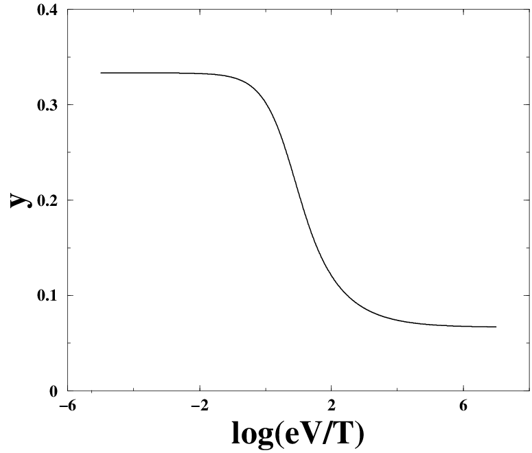
Let us now discuss the main features of the function . In agreement with symmetry requirements is an odd function of the voltage (the even correlator is proportional to the absolute value of voltage), and vanishes at equilibrium. The zero temperature result (high voltage limit) has already been obtained by means of the scattering states approach for single-channel systems [4], and later generalized by means of Random Matrix Theory (RMT) to multi-channel systems (chaotic and diffusive) [18]. In our derivation we do not assume the applicability of RMT [19]. Our result covers the whole temperature range. We obtain that at low temperatures the third order cumulant is linear in the voltage
| (47) |
At high temperatures the electrons in the reservoirs are not anymore in the ground state, so the correlations are partially washed out by thermal fluctuations. One may then expand , eq. (II.1), in a series of . The leading term in this high temperature expansion is linear in the voltage
| (48) |
Note that although thermal fluctuations enhance the noise (compared with the zero temperature limit), eqs.(47) and (48) differ only by a numerical factor. The experimental study of (and higher odd cumulants) provides one with a direct probe of non-equilibrium behavior, not masked by equilibrium thermal fluctuations.
II.2 Strong Inelastic Collisions
In our analysis so far we have completely ignored inelastic collisions among the electrons. This procedure is well justified provided that the inelastic length greatly exceeds the system’s size. However, if this is not the case, different analysis is called for. To understand why inelastic collisions do matter for current fluctuations, we would like to recall the analysis of for a similar problem. The latter function is fully determined by the effective electron temperature. Collisions among electrons, which are subject to an external bias, increase the temperature of those electrons. This, in turn, leads to the enhancement of , cf. Refs. [20, 21]. In the limit of short inelastic length
| (49) |
the zero frequency and zero temperature noise is
| (50) |
In the present section we consider the effect of inelastic electron collisions on . We assume that the electron-phonon collision length is large, , hence electron-phonon scattering may be neglected. The Hamiltonian we are concerned with is
| (51) |
The Coulomb interaction among the electrons is described by
| (52) |
where
| (53) |
We need to deal with the effect of electron-electron interactions in the presence of disorder and away from equilibrium. Following Ref. [23] one may introduce an auxiliary bosonic field
which decouples the interaction in the particle-hole channel. Now the partition function (eq. (29)) is a functional integral over both the bosonic fields and ,
| (57) |
The action is
| (58) | |||
| (59) | |||
| (60) |
It is convenient to perform a “gauge transformation” [23] to a new field
| (61) |
Introducing the long derivative
| (62) |
one may write the gradient expansion of eq. (60) as
| (63) | |||
At this point the vector that determines the transformation (61) is arbitrary. The saddle point equation for of the action (63) is given by the following equation
| (64) |
Let us now choose the parameterization
| (65) |
where represents fluctuation around the saddle-point
| (66) |
Eq. (66) implies that the solution of the saddle point equation (64), determines as a functional of . We do not know, though, how to solve it. Instead we average over the eq.(64). The solution of this averaged equation, denoted by , is determined by:
| (67) |
where the r.h.s. is given by
| (68) |
Since () is not a genuine saddle point of the action there is coupling between the fields and in the quadratic part of the action. However the coupling constant between those fields is proportional to the gradient of the distribution (cf. eq.(II.2)). Therefore this term can be treated as a small perturbation.
Taking variation of the action with respect to , , we obtain the following gauge, determining :
| (69) |
where
| (70) |
Though we have failed to find the true saddle point the linear part of the action expanded around () is zero. It is remarkable to notice that under conditions (II.2) eq.(67) becomes a quantum kinetic equation [24] with the collision integral being . Coming back to our calculations we note that the correlation function of current fluctuations is a gauged invariant quantity (does not depend on the position of the Fermi level). This means that momenta do not contribute to such a quantity [22]. In this case the Coulomb propagator is universal, i.e. does not depend on the electron charge. The fact that we address gauge invariant quantities allows us to represent the generating functional in terms of the fields and (rather than and ), as in Ref [23].
| (71) |
Here we define
| (72) |
where the expansion , is in powers of ; the power () is given by
| (73) |
| (74) |
| (75) |
From eq.(72) we obtain the gauge field correlation function
| (76) |
where
Using eqs.(76,II.2) we rewrite eq.(II.2) for the quasi-one-dimensional wire as:
| (80) | |||
| (81) |
The total number of particles and the total energy of the electrons are both preserved during electron-electron and elastic electron-impurity scattering. The collision integral, eq.(II.2), satisfies then
| (82) |
| (83) |
We now consider the limit . The solution of eq.(67) assumes then the form of a quasi-equilibrium single-particle distribution function
| (84) |
Here is the total energy of the electron, and
is the electrostatic potential and is the
effective local temperature of the electron gas.
To find the electrostatic potential
we employ eq. (82). To facilitate our
calculations we further assume that conductance band is symmetric
about the Fermi energy and that the spectral density of
single-electron energy levels is constant.
Integration over the energy, eq.(82) yields
| (85) |
Solving eq.(85) under the condition that the voltage difference at the edges of a constriction is , we find
| (86) |
Multiplying eq. (80) by energy and and employing eq.(83) we obtain an equation
| (87) |
The boundary condition of eq.(87) is determined by the temperature of the electrons in the reservoirs. Combining eqs.((86) and (87)) we find the electron temperature in two opposite limits:
Eqs.((84), (86) and (II.2) determine the function uniquely. We now replace the right-corner element of the matrix (i.e. , cf. eq.(66)) by its average value .
To calculate under conditions of strong electron-electron scattering (eq. (49)) one needs to replace the operators and in eq. (II.1) by their gauged values
| (91) |
where the averaging is taken over the entire action and the Gaussian weight function for , as in eq. (57). Here we define (cf. eqs.(35), (36) with eqs. (92),(93))
| (92) |
| (93) |
where the “long derivative”, , is presented in eq.(62). In order to actually perform the functional integration over the matrix field we use the parameterization of eq. (65). We need to find the Gaussian fluctuations around the saddle point of the action (73,74,75). Though we did not find the exact saddle point, the expansion of around works satisfactorily. The coupling between the fields and which appears already in the Gaussian (quadratic) part is small, since it is proportional to the gradient of the distribution function:
| (94) |
Here the upper index refers to the power of the fields; the lower refers to the power of fields in the expansion. Considered as a small perturbation, does not affect the results.
The more dramatic effect on the correlation function arises from the non-Gaussian part of the action, eqs. (74,75) (by this we mean non-Gaussian terms in either or ). After integrating over the interaction an additional contribution to the Gaussian part (proportional to ) of the action arises. To find the effective action we average over the interaction [16]. One notes that
| (95) |
(where, again, refers to the component of the action, eq.(74), that has zero power of the fields and one power of the field). In addition, due to the choice of the gauge, eq.(II.2), and the condition (), the averaging over does not generate terms linear in in the effective action:
| (96) |
Combining eqs. (95 and 96) we find that the effective action acquires an additional contribution:
| (97) |
The general form of the effective action is rather complicated, however for the low frequency noise only diagonal part of the action matters:
| (98) |
Here the operator
| (99) | |||
is a linearized collision integral, i.e. a variation of the collision integral (II.2) with respect to the distribution function. Substituting eqs.(92 and 93) into eq.(91) and calculating the Gaussian integrals with the action (II.2), we find
| (100) |
where the “inelastic diffusion” propagator, , is the kernel the equation
| (101) |
For weak electron-electron scattering the collision integral is small, yielding the standard propagator of the diffusion equation, D (cf. eq. 43). In the presence of strong electron-electron scattering the collision integral dominates eq.(101). In this limit we evaluate the leading asymptotic behavior for (). On scales longer than the inelastic mean free path the distribution function has a quasi-equilibrium form
| (102) |
where
| (103) |
The values of the local temperature and electro-chemical potential can fluctuate. To find the correlations of these fluctuations we consider the equation (with the same Kernel as in eq.(101))
| (104) |
Integrating equation (104) with respect to energy and using the particle-conservation property of the collision integral (eqs.(82)) we find:
| (105) |
Using energy conservation (eq. 83) we find
| (106) |
Combining eqs. (105) and (106) we find:
| (107) |
Evaluating explicitly we find that the third order current cumulant is
| (108) |
At high temperatures (cf. eq.II.2) one obtains
| (109) |
while at low temperatures
| (110) |
Our analysis was performed for a simple rectangular constriction. However, our results hold for any shape of the constriction, provided it is quasi-one dimensional (we have considered a single transversal mode only).
III COMPARISON WITH THE KINETIC THEORY OF FLUCTUATIONS
As was mentioned in Section I.3 the applications of the kinetic equation in the study of high order cumulants is not straight forward. To compare our microscopic quantum mechanical calculation with the semi-classical Boltzmann-Langevin scheme we consider the diagrams for the pair and third order correlation function, depicted in Fig.(3).
The diagram in Fig. (3-b) corresponds exactly to the results obtained above in the framework of the -model formalism. Indeed, evaluating this diagrams, we recover the results (45) and (100). Comparing Fig. (3-b) with diagram (3-a) (the latter determines the correlator of Langevin sources), we conclude that the third cumulant corresponding to Fig. (3-b) can be expressed in the form
| (111) |
Indeed, the block on the right hand side of the diagram corresponds to the pair correlation function of random fluxes, while the left part can be obtained by functional differentiation of the diagram (3-a) with respect to the function . This justifies the regression scheme proposed recently by Nagaev [26]. Diagram (3-a) for the pair correlation function is local in space; the diagram for the third order correlator is not. Despite this non-locality the use of the Langevin equation (with non-local random flux) remains convenient; in that case the correlation function of the random fluxes needs to be calculated from first principles. This is somewhat analogous to the description of mesoscopic fluctuations through the Langevin equation, proposed by Spivak and Zyuzin [25].

The vector vertices represent the current operators, while collisions with static disorder correspond to the Hikami box (). , where is the single-electron distribution function. D is the diffuson.
Following Ref[17] the revisited version of the kinetic theory of fluctuations has been proposed by Nagaev [26]. He has noticed that for a diffusive system there exists a regression scheme of high order cumulants, expressed in terms of pair correlators [27]. However, a truly classical theory addressing high moments of noise needs to be taken on the same footing as the Boltzmann-Langevin theory, i.e. without appealing to quantum mechanical diagrammatics. Close inspection of the diagrams depicted in Fig. 3 and the dimensionless parameter by which corrections are small implies that the regression recipe (eq. III) has the same range of applicability as the Boltzmann-Langevin scheme itself.
As a simple example of a classical problem for which the regression procedure can be applied, we consider the following simple model[6]. A heavy molecule of mass and cross-section is embedded in a gas of light classical particles. The gas consists of particles of mass , in thermal equilibrium with temperature . It is enclosed in a narrow tube of volume . The fluctuating velocity of the molecule here is the analogue of the fluctuating electron distribution function . The collisions of the molecule with the light particles is the counterpart of the electron’s scattering on the random disorder. The motion of the molecule is governed by Newton law
| (112) |
Here is the velocity and is the force acting on the molecule. The latter can be calculated from
| (113) |
where and are the fluctuating distribution functions of particles on the left and on the right sides of the system respectively. Since the time between two consecutive collisions is much shorter than the relaxation time of the molecule () one can average over fast collisions while considering the relaxation dynamics of the heavy molecule:
| (114) |
To find the various velocity correlation functions, one needs to know the corresponding correlation functions of the random forces. Using the fact that the equilibrium fluctuations of the distribution function in a Boltzmann gas are Poissonian ([7], Section 114) and neglecting the small velocity relatively to , one finds the pair correlation function
| (115) |
Eq. (115) yields the correct value for the thermal fluctuations . To find the higher order correlations of the random force one has to take into account the dependence of the force on the velocity of the molecule. We expand eq.(113) up to second order in . After averaging over all possible pair correlations (such as and ) we obtain
| (116) |
Here denotes all permutation over (). The triple force correlator was reduced to pair correlators only. Bearing in mind the analogy between and on one hand, and the scattering of the electrons on the disorder and the scattering of the molecule by light particles on the other hand, we note that the reduction of the third order cumulant of the random forces to the pair correlation functions is similar in both cases.
We finally come back to the question of whether it is possible to calculate high order cumulants employing the classical kinetic equation (Boltzmann-Langevin) rather than resorting to the diagrammatic reduction scheme depicted above. To be able to answer this question we first note that the applicability of the kinetic theory requires that both . Here is the correlation time for the current signal and is the dimensionless conductance. For non-interacting electrons Onsager relation and Drude formula yield , where is the transport time. It follows that the condition
| (117) |
must be satisfied. The reason for theses inequalities are first, that needs to be large in order for quantum interference effects to be negligible. Secondly, the value needs also to be small; the transport equation is applicable for times longer than the duration time of an individual collision , (). For a degenerate electron gas the uncertainty relation requires that [28, 29].
We now evaluate the relative magnitude of, e.g., the fourth and the second cumulants. We consider the ratio
| (118) |
where denotes the irreducible part of the correlator. At equilibrium
| (119) |
As we see, for the kinetic theory to be valid, the value of the parameter needs to be small. But this is exactly the parameter () by which the high order correlation functions are smaller than the lower ones (cf. eq.117). In other words, the evaluation of high order cumulants goes beyond the validity of the standard Boltzmann-Langevin equation. This is why we have to resort to the diagrammatic approach: either to justify the reduction of high order cumulants to pair correlators, or, alternatively, to introduce non-local noise correlators in the Boltzmann-Langevin equation.
IV COUNTING STATISTICS
So far we have studied the second and third order cumulants. In the present section we discuss the whole distribution function of the low frequency electron current (so-called counting statistics). The zero temperature limit had been studied by Levitov et. al. [18]. The full temperature regime was addressed by Nazarov[31]. Here we present a different derivation based on the -model approach.
Being a stochastic process, the charge transmission can be characterized by the probability distribution function (PDF) of the probability for electrons to pass through the constriction within the time window . In practice it is more convenient to work with the Fourier transform of the PDF, the characteristic function
| (120) |
Below we evaluate for the case of elastic scattering. By expanding the logarithm of characteristic function over its argument we can find the cumulants (irreducible correlation functions) of a transmitted charge
| (121) |
For the problem of diffusive junction the disorder average characteristic function can be represented as:
| (122) |
where the external source is given by
The applied bias enters the problem through boundary conditions on at the edges of the constriction:
and is defined by eq.(39).
Inasmuch as we are not interested in spatial correlations, the external source term is a function of time only. Therefore, by performing the transformation
| (126) |
one gets:
| (127) |
and the boundary conditions change correspondingly:
| (128) |
with
| (129) |
We use the saddle point approximation to calculate the characteristic function, Eq. (122). In the presence of an external potential the minimum of the action, eq. (IV), satisfies
| (130) |
Let us define a parameter that can roughly be regarded as “the number of attempts per channel”, . We will focus on the case where the time window is much larger than the Thouless time and the conductance . Inside the region eq. (IV) becomes (up to the corrections
| (131) |
This can be represented in the form resembling a current conservation law
| (132) |
where the current is defined as
| (133) |
The solution of Eq. (132), can be written as
| (134) |
and from the boundary conditions (eq. IV) it follows that
| (135) |
One may show that the anticomutator of the matrix with vanishes
| (136) |
Based on this property, we can show that the following statements do hold:
(1) The square of the matrix is still equal to unity
| (137) |
(2) The determinant of the matrix satisfies
| (138) |
(3) The trace of the matrix is equal to zero
| (139) |
(4) The trace of the matrix is zero
| (140) |
(5) The square of the matrix is proportional to the unit matrix
| (141) |
where is given by (there is small discrepancy with the result obtained in Ref.[31])
Using these properties we find the disorder averaged counting statistics
| (143) |
The zero temperature limit coincides with the results derived previously by Lee et. al.[18].
At finite temperatures we find:
| (144) |
It is worthwhile to note that the value of agrees with the one obtained in Ref.[26]. As we see the counting statistics of the current in a disordered wire is not Gaussian. Remarkably, all the information contained in the counting statistics can be extracted from the pair correlation function (of the distribution function), eq.(I.3).
Finally we would like to discuss the role of inelastic electron-phonon scattering. As has been already realized [1], such an interaction suppresses shot noise. Moreover, based on our approach, one can show that in the limit of (macroscopic conductor) the current fluctuations are Gaussian (to leading order in ). To show this, we repeat our analysis concerning . We find that eq. (100) still holds, but the distribution function and the inelastic diffusion propagator need to be calculated taking electron-phonon collisions into account. In the presence of both electron-electron and electron-phonon interaction one obtains
| (145) |
(cf. eq.67) where is the linearized electron-phonon collision integral. The inelastic diffuson (cf. eq.101) is now determined by
| (146) |
In the limit fluctuations of the chemical potential is the only long-range propagating mode in the problem (no fluctuations of the along the system). Solving eqs.(145, IV and 100) we find that vanishes as . A conductor longer than the electron-phonon length () can be viewed as a number () of resistors connected in series. The current fluctuations of a single resistor are given by eq.(143) and would render the corresponding voltage fluctuations. Since the fluctuations at different resistors are uncorrelated (local fluctuations in the chemical potential do not change the resistance significantly) the large number of the resistors results in Gaussian current fluctuations. By contrast, temperature fluctuations (in the case of solely electron-electron interactions) have long distance correlations, and give rise to non-Gaussian fluctuations.
Acknowledgments
The authors wish to thank M. Reznikov and Y. Levinson for inspiring discussion and A. Kamenev for his critical comments in the earlier stages of this work. This work was supported by GIF foundation, the Minerva Foundation, the European RTN grant on spintronics, by the SFB195 der Deutschen Forschungsgemeinschaft, and by RFBR gr. 02-02-17688.
References
- [1] Ya. M. Blanter, M. Büttiker Physics Reports 336, 2, (2000).
- [2] A.Ya. Shulman Sh.M. Kogan Sov. Phys. JETP 29 , 3 (1969).
- [3] S.V. Gantsevich, V.L. Gurevich and R. Katilius Sov. Phys. JETP 30, 276 (1970).
- [4] L.S. Levitov and G.B. Lesovik Sov. Phys. JETP Lett. 58, 230, (1993).
- [5] L.S. Levitov and M. Reznikov “Electron shot noise beyond the second moment” cond-mat/0111057.
- [6] M. Reznikov, private comm.
- [7] L.D. Landau and E.M. Lifshitz Statistical Mechanics, (Pergamonn Press, Oxford, 1980), Pt. 1.
- [8] L.S. Levitov, H. Lee and G.B. Lesovik Journal of Math. Phys. 37, 4845 (1996).
- [9] I. Klich “Full Counting Statistics: An elementary derivation of Levitov’s formula” cond-mat/0209642, to appear in these proceedings.
- [10] L.V. Keldysh JETP 20, 1018 (1965).
- [11] We note that even physical observables corresponding to the second current correlator may be associated with different current correlation functions, such as symmetrised, antisymmetrzied or combinations thereof. For discussion of this point see G.B. Lesovik and R. Loosen, Pism’ma Zh. E’ksp. Teor. Fiz. 65, 280 (1997) [JETP Lett. 65, 295, (1997)]; U. Gavish, Y. Levinson and Y. Imry Phys. Rev. B. 62, R10637 (2000).
- [12] R de-Piccioto, M. Reznikov, M. Heiblum, V. Umansky, G. Bunin and D. Mahalu Nature 389, 6647 (1997).
- [13] L. Saminadayar, D. C. Glattli, Y. Jin and B. Etienne Phys.Rev. Lett. 79, 2526 (1997).
- [14] E.M. Lifshitz and L.P. Pitaevskii Physical Kinetics (Pergamonn Press, Oxford, 1981).
- [15] M. Lax Rev. Mod. Phys. 32, 25 (1960).
- [16] D.B. Gutman and Yuval Gefen “Shot noise at high temperatures”, cond-mat/0201007
- [17] D.B. Gutman and Y. Gefen Phys. Rev. B. 64, 205317 (2001).
- [18] H. Lee, L.S. Levitov and A.Yu. Yakovets Phys. Rev. B 51, 4079, (1995).
- [19] for the discussion of application of random-matrix theory to shot noise see M. J. M. de Jong, C. W. J. Beenakker in ”Mesoscopic Electron Transport,” edited by L.L. Sohn, L.P. Kouwenhoven, and G. Schoen, NATO ASI Series Vol. 345 (Kluwer Academic Publishers, Dordrecht, 1997).
- [20] K.E. Nagaev Phys. Rev. B 52, 4740, (1995).
- [21] V.I. Kozub and A.M. Rudin Phys. Rev. B, 52, 7853, (1995).
- [22] A.M. Finkel’stein Physica B 197, 636 (1994).
- [23] A. Kamenev, A. Andreev Phys. Rev. B 60, 2218 (1999).
- [24] A. Schmid Z. Physik 271 251 (1974); B.L. Altshuler and A.G. Aronov JETP Lett. 30 483 (1979).
- [25] A.Ju. Zyuzin, B.Z. Spivak, Zh. Eksp. Theor. Fiz. 93, 994 (1987) (Sov. Phys. JETP 66, 560 (1987)).
- [26] K. E. Nagaev Phys. Rev. B 66, 075334 (2002).
- [27] Recently the regression procedure has been applied for a closed disordered cavity: K.E. Nagaev, P. Samuelsson, S. Pilgram “Cascade approach to current fluctuations in a chaotic cavity”, cond-mat/0208147
- [28] R. Peierls Helv. Phys. Acta 7, Suppl. 2, 24 (1934).
- [29] As a side remark, we note that if the condition is not satisfied the deviation from the kinetic theory may be substantial. In particular the renormalization of conductance by electron-electron interaction (Altshuler-Aronov effect) is pronounced when is small[30].
- [30] B.L. Altshuler and A.G. Aronov in Electron Electron interaction in the disordered metals, (Elsevier Science Publishers B.V., New-York, 1985).
- [31] Yu. V. Nazarov Ann. Phys. (Leipzig) 8, Spec. Issue, 193 (1999). We believe that the result in this paper contains a small error.