Quantum Brownian motion and
its conflict with the second law

Introduction. There are not two fundamental theories of nature, quantum mechanics and thermodynamics. There is only one: quantum mechanics, while thermodynamics must emerge from it. The universal character of equilibrium thermodynamics led to the general expectation that in one way or another, thermodynamics will apply to the full quantum domain landau. Few people have taken the painful road to check this emergence, yet this is what we have set out to do. Here we discuss the results for quantum Brownian motion that have been presented  ANQBMprl; NAlinw and were discussed in the scientific literature AIP.

Brownian motion has numerous applications in condensed matter physics klim; weiss; risken; leggett, atomic physics klim, quantum optics and chemistry gardiner. Some realizations involve weak coupling with the thermal bath gardiner. However, there are well-known experimental situations, which are essentially far from the weak-coupling regime. Here standard thermodynamics may not apply. The main example of this is the case of weak links between superconductive regions, the so-called Josephson junctions, in their overdamped regime van; likho, where the relevant ranges of parameters were achieved already twenty years ago. Even in quantum optics, which has often been satisfactorily described by weak-coupling theories gardiner, there are recent experiments showing the necessity for moderate and strong coupling approaches  oe.

The Hamiltonian. We consider an ‘ideal gas’ of non-interacting harmonic oscillators coupled to a bath. For the total Hamiltonian ${\cal H}_{\rm tot}={\cal H}+{\cal H}_{B}+{\cal H}_{I}$ we thus assume weiss

with ${\cal H}$ describing the particle, ${\cal H}_{B}$ the bath, and ${\cal H}_{I}$ the interaction.

The bath is assumed to have uniformly spaced modes $\omega_{i}=i\Delta,\qquad i=1,2,3,\cdots$. The thermodynamic limit for the bath is taken by sending $\Delta\to 0$, which induces relaxational behavior. For the couplings we choose the quasi-Ohmic Drude-Ullersma spectrum, where weiss $J(\omega)=\frac{1}{2}{\pi}\sum_{i}({c_{i}^{2}}/{m_{i}\omega_{i}})\delta(\omega-\omega_{i})={\gamma\omega\Gamma^{2}}/(\omega^{2}+\Gamma^{2})$, where $\gamma$ is the damping constant. We shall assume that the Debye cutoff $\Gamma$ is large.

We describe an ensemble of closed total systems with conserved energy, except for the periods when work is done on it by externally changing $m$ or $a$. We take as initial density matrix the Gibbs distribution $\exp(-\beta{\cal H}_{\rm tot})/Z_{\rm tot}$, with $Z_{\rm tot}$ the partition sum.

Equilibrium state. In Gibbsian equilibrium of the total system the free energy reads $F_{\rm tot}(T,\gamma)=F_{B}(T,\gamma=0)+F_{p}(a,\gamma,\Gamma,m,T)$. The free energy of the bath itself,

is of order $1/\Delta$, showing the extensivity of the bath. The Brownian particle adds to this

It contains three characteristic, temperature independent of frequencies. For small $\gamma$ (underdamping) they read: $\omega_{1,2}=\pm i\omega_{0}+{\gamma}/{2m}$, $\omega_{3}=\Gamma-{\gamma}/{m}$. On the other hand, for strong damping $\gamma^{2}\gg am$, $\omega_{1}={a}/{\gamma}$, $\omega_{2}=({\gamma}/{m})(1-{am}/{\gamma^{2}})$, $\omega_{3}=\Gamma-{\gamma}/{m}$.

Effective temperatures. We shall now study two objects, $T_{x}=a\langle x^{2}\rangle$ and $T_{p}=\langle p^{2}\rangle/m$, that would in classical equilibrium be equal to $T$ and which we shall interpret below as effective temperatures. As in the classical situation, it holds that $T_{x}=2a{\partial F_{p}}/{\partial a}$, $T_{p}=-2m{\partial F_{p}}/{\partial m}$. For $\gamma\to 0$ one gets the weak-coupling result known from textbooks, $U\equiv\frac{1}{2}T_{x}+\frac{1}{2}T_{p}=T_{x}=T_{p}={\frac{1}{2}\,{\mathchar 22\mkern-7.0muh}\omega_{0}}\coth\frac{1}{2}{\beta\,{\mathchar 22\mkern-7.0muh}\omega_{0}}$, with $\omega_{0}=\sqrt{a/m}$. At large $T$ one gets

At low $T$ and for strong damping one has

The fact that $T_{p}\geq T_{x}>0$ at $T=0$ is related to the quantum nature of the problem.

Generalized thermodynamic formulation. The Wigner function has a quasi-Gibbsian expression, since there occur two temperature-like variables,

The Boltzmann entropy of momentum and coordinate is

while the von Neumann entropy reads weiss $S_{vN}=(v+\frac{1}{2})\ln(v+\frac{1}{2})-(v-\frac{1}{2})\ln(v-\frac{1}{2})$, with $v={\Delta p\,\Delta x}/{\,{\mathchar 22\mkern-7.0muh}}=\sqrt{{\langle p^{2}\rangle\langle x^{2}\rangle}}/{\,{\mathchar 22\mkern-7.0muh}}=\sqrt{{mT_{p}T_{x}}}/\,{\mathchar 22\mkern-7.0muh}\sqrt{a}$. The first terms in its large $v$-expansion, $S_{vN}=\ln v+1$, coincide with the total Boltzmann entropy $S_{B}=S_{p}+S_{x}$.

Internal energy and interaction energy. The energy of the central particle reads $U=\langle{\cal H}\rangle=\frac{1}{2}T_{p}+\frac{1}{2}T_{x}$. The energy of the cloud of bath modes that surround the particle is $U_{\rm int}=U_{\rm tot}-U_{B}(\gamma=0)-U=U_{p}-U=\Gamma{\partial F_{p}}/{\partial\Gamma}$. At high temperatures one has $U=T+{\beta\,{\mathchar 22\mkern-7.0muh}^{2}}(2a+\gamma\,\Gamma)/24m$, $U_{\rm int}={\beta\,{\mathchar 22\mkern-7.0muh}^{2}\gamma\,\Gamma}/{24m}$. Since the energy of the cloud involves $\,{\mathchar 22\mkern-7.0muh}$, it is a quantum effect. At low temperatures one has, if $\Gamma$ is large, $U_{\rm int}={\,{\mathchar 22\mkern-7.0muh}\gamma}/{2\pi m}+{\cal O}(T^{4})$.

Implementation of the first law. Given the Hamiltonian ${\cal H}(p,x)$ of the subsystem, its energy is $U=\langle{\cal H}\rangle=\int{\rm d}p{\rm d}x{\cal H}(p,x)W(p,x)$, where $W$ is the Wigner function of the subsystem. When we change a system parameter, the energy changes as ${\rm d}U={\rm d}\int{\cal H}W=\int{\cal H}\,{\rm d}W+\int W\,{\rm d}{\cal H}\equiv\,\,{\mathchar 22\mkern-9.0mu{\rm d}}{\cal Q}+\,\,{\mathchar 22\mkern-9.0mu{\rm d}}{\cal W}$. The first term represents the variation due to the statistical redistribution of the phase space, which we identify with the change in heat $\,\,\,{\mathchar 22\mkern-9.0mu{\rm d}}{\cal Q}$. The last term results from the change in the Hamiltonian, so it is a mechanical, non-statistical object, which we associate with the work $\,\,\,{\mathchar 22\mkern-9.0mu{\rm d}}{\cal W}$ done by external sources.

Generalized free energy and the second law. The definition of the effective temperatures admits a thermodynamical interpretation. The free energy $F$ for a two-temperature system is defined as  1 $F=U-T_{p}S_{p}-T_{x}S_{x}=-\frac{1}{2}T_{p}\ln mT_{p}-\frac{1}{2}T_{x}\ln({T_{x}}/{a})$. For adiabatic changes in $m$ or $a$ one has ${\rm d}F=-S_{x}{\rm d}T_{x}-S_{p}{\rm d}T_{p}+\,\,{\mathchar 22\mkern-9.0mu{\rm d}}{\cal W}$, with work $\,\,{\mathchar 22\mkern-9.0mu{\rm d}}{\cal W}=\langle{\partial{\cal H}}/{\partial m}\rangle{\rm d}m+\langle{\partial{\cal H}}/{\partial a}\rangle{\rm d}a=-T_{p}{{\rm d}m}/{2m}+T_{x}{{\rm d}a}/{2a}$. Due to the first law this yields the second law for situations with two temperatures, $\,\,{\mathchar 22\mkern-9.0mu{\rm d}}{\cal Q}=T_{p}{\rm d}S_{p}+T_{x}{\rm d}S_{x}$, in close analogy with those proposed recently for nonequilibrium glassy systems 1 and black holes Nbh. Notice that $F$ pertains to the particle alone, and does not satisfy Gibbsian thermodynamics, while the Gibbsian $F_{p}$ of Eq. (3), relates to the whole equilibrium system, i.e., to the particle and the cloud of bath modes around it. There are many physical systems, such as a Josephson junction strongly coupled to the electromagnetic field, where the natural object to study is $F$, relating to properties of the junction only.

Violation of the Clausius inequality at low $T$. The Clausius inequality $\,\,{\mathchar 22\mkern-9.0mu{\rm d}}{\cal Q}\leq T{\rm d}S_{vN}$ is one of the formulations of the second law. At $T=0$ it says that no heat can be taken from the bath, at best heat can go from the subsystem to the bath.

When we change $a\to a+{\rm d}a$, $\,\,{\mathchar 22\mkern-9.0mu{\rm d}}{\cal Q}$ is of order $-T^{2}{\rm d}a$, while $T{\rm d}S_{vN}$ is of order $-T{\rm d}a$. In the case ${\rm d}a>0$, where an amount of work $\,\,{\mathchar 22\mkern-9.0mu{\rm d}}\,{\cal W}_{\rm rev}\sim{\rm d}a$ is done on the system, the Clausius relation is thus violated at low $T$. Likewise one can consider the variation of the (effective) mass $m$. Here one has $\,\,{\mathchar 22\mkern-9.0mu{\rm d}}{\cal Q}=\,{\mathchar 22\mkern-7.0muh}\gamma\,{\rm d}m/{2\pi m^{2}}$. Now there is a transfer of heat even if the bath temperature is zero. Thus, violation of the Clausius inequality is even stronger in this case. This situation with $\,\,{\mathchar 22\mkern-9.0mu{\rm d}}\,{\cal W}_{\rm rev}<0$ corresponds to the work performed by the system on the environment. That the heat comes from the cloud of bath modes, is confirmed by the fact that $\,\,{\mathchar 22\mkern-9.0mu{\rm d}}{\cal Q}_{\rm rev}=-{\rm d}U_{\rm int}$.

Violation of the Landauer bound for information erasure. A further aspect is the squeezing of phase space and entropy, relevant for computing in the quantum regime. We have shown that the so-called Landauer bound $-\,\,{\mathchar 22\mkern-9.0mu{\rm d}}{\cal Q}\geq kT\,\ln 2$ for the minimal energy dispersion when erasing one bit of information is violated in a similar manner ANQBMprl. This connection arises because the Landauer bound is just based on the Clausius inequality.

Dynamics from a non-equilibrium state. Energy oscillation at low $T$. We consider the dynamical evolution of a system initially in equilibrium characterized by a spring constant $a_{0}$, which at $t=0$ is instantaneously changed to $a_{1}=a$. These parameters are connected as $a_{0}=(1-\alpha_{0})a$ and we assume that $|\alpha_{0}|\ll 1$. For strong damping one has for the energy of the subsystem $U(t)=U(\infty)+(\,{\mathchar 22\mkern-7.0muh}a\alpha_{0}/2\pi\gamma)f_{1}(at/\gamma)$. The behavior of $f_{1}(\sigma)$ at different temperatures is presented in Fig. 1a. For $\alpha_{0}>0$ it says that, after initially energy has been put on the particle by the change of $a_{0}\to a>a_{0}$, this energy leaks away into the bath. At low $T$, however, too much leaks away, and a part has to come back. This “bouncing” is familiar of the noise correlator, which behaves like $f_{1}$.

Entropy production. The rate of production of Boltzmann entropy is found after a lengthy identification of its flux. The result can be negative at moderate $T$ NAlinw. For $T=0$ and strong damping one has with $\sigma=at/\gamma$ and $\sigma_{min}=0.879$: ${{\rm d}_{i}S_{x}}/{{\rm d}t}\sim+\alpha_{0}^{2}(\sigma-{\sigma_{\rm min}})(\sigma-{\sigma_{\rm min}}+\varepsilon)$, where $\varepsilon=am/\gamma^{2}$. This is negative for ${\sigma_{\rm min}}-\varepsilon<\sigma<{\sigma_{\rm min}}$, or $\Delta t=m/\gamma$, the characteristic timescale of the momentum.

Smooth changes of the spring constant. Let us now consider the case where, starting from the equilibrium state $a(-\infty)=a$, the spring constant $a(t)=[1-\alpha(t)]a$, is slightly changed ($|\alpha(t)|\ll 1$) in a smooth way. The rate of work added to the system is ${{\rm d}{\cal W}}/{{\rm d}t}={{\rm d}{\cal W}_{\rm rev}}/{{\rm d}t}+{{\rm d}\Pi}/{{\rm d}t}$, with the adiabatic (‘reversible’) and dispersed contributions

where $\tau=\gamma\,t/2m$ and $C_{x}$ a function like $f_{1}$ of Fig. 1a. Integrating over the full change (the whole region where $\alpha^{\prime}\neq 0$) one confirms that the dispersion for a completed, cyclic change ($\alpha_{i}=\alpha_{f}$) of system parameters is nonnegative, the Thomson formulation of the second law ANthomson. It is also nonnegative for noncyclic ($\alpha_{i}\neq\alpha_{f}$) but completed changes.

Energy dispersion. If $\alpha(\tau)=\alpha_{m}h(\Omega t)$, with $\Omega$ a slow rate of change, and $\gamma$ is large, expansion in $\Omega$ is possible. Omitting numerical factors one gets the structure

The full integral is always positive and for moderate $T$ the first term is dominant. However, for small $T$ the term $h^{\prime}h^{\prime\prime}$ may imply that ${{\rm d}\Pi}/{{\rm d}t}$ is negative. This is a firm statement, also valid when starting in equilibrium, since work is the energy added to the total system. It is the more surprising since the relevant domain the characteristic timescale of the change of $a$, $1/\Omega<\,{\mathchar 22\mkern-7.0muh}^{2}/(\gamma T^{2})$, may exceed all other timescales, including the quantum timescale $\,{\mathchar 22\mkern-7.0muh}/T$, so that applicability of thermodynamics was to be expected.

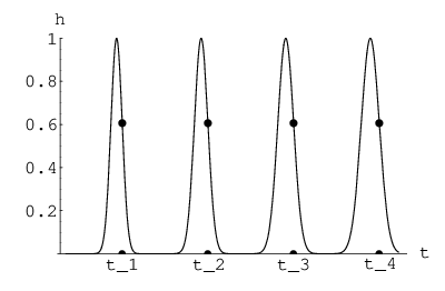
Perpetuum mobile with many work extraction cycles. The $h^{\prime}h^{\prime\prime}$ term can cause extraction of work. Let there be ${\cal N}$ non-overlapping Gaussians, $h(x)=\exp(-\frac{1}{2}x^{2})$, as depicted in Figure 1b. Cycles are the intervals $t_{i}<t<t_{i+1}$ ($i\geq 1$). Each new cycle is slower than the previous one, $\Omega_{n+1}<\Omega_{n}$. One can make a total number ${\cal N}\sim 1/T$ of cycles with equal yield, where ${\cal N}$ is parameterized by $v$, and total yield

with $I_{1}=\frac{1}{2}\sqrt{\pi}$, $I_{3}=3\sqrt{\pi}/4$. The minus sign of ${\cal W}_{\rm tot}$ indicates that work is performed by the system on the environment. This is possible because, in order to make the extraction cycles, one had to start from the equilibrium state $\alpha(-\infty)=0$ and change $\alpha$ up to $\alpha(t_{1})$. In this first part the energy dispersion was $\Pi(t_{1})=+{{\alpha_{\rm m}^{2}}}{\,{\mathchar 22\mkern-7.0muh}\gamma}\Omega_{1}^{2}/24\pi a\,\,>\,\left|{\cal W}_{\rm tot}\right|$.

Feasibility. The harmonic oscillator can be interpreted as an LC circuit klim-rev. $x$ may correspond to the charge $Q$ on a capacitor, $1/a$ to its capacitance $C$, $m$ to an inductance $L$, $p$ to a phase $\Phi$, $\gamma$ to a resistance $R$, and $\eta(t)$ to a random electro-motoric force. In this setup there should be nothing difficult in varying $L\sim m$ or $C\sim 1/a$. We have proposed to test the violation of the Clausius inequality in mesocopic linear circuits NArlc. This amounts to measuring $\langle\delta Q^{2}\rangle$, $\langle\delta\Phi^{2}\rangle$ and the produced work. The conditions to do this experiment were reached 20 years ago, and one of the quantities, $\langle\delta Q^{2}\rangle$, was measured already and agrees perfectly with the theoretical predictions  w1; flabby.

Has thermodynamics been violated? Let us recall that our results hold also for $N$ non-interacting Brownian particles in a bath. Our conclusion is that thermodynamics does not always work when, in the quantum regime, one considers the Brownian particle in its reduced Hilbert space, thus summing out the bath. We should admit that at low enough $T$ the interaction energy between system and bath becomes relevant, since the damping constant is fixed. In a very strict definition of thermodynamics one may claim that there is no reason why thermodynamics had to apply.

For this reason our surprising findings of the breakdown of the Clausius inequality can in principle be viewed as results outside the domain of applicability of thermodynamics. However, the negativity of the Boltzmann entropy production sets in already at moderate $T$, more or less in the same domain where energy initially put on the particle starts to dissipate to the bath in a non-monotonic fashion, even in limit of large damping.

Our second effect in that regime, the presence of many work extraction cycles (“perpetuum mobile”) involves only the energy budget of the total system, and should be more surprising. However, when starting in an equilibrium state and counting all the energy, the total dispersion is positive, as demanded by an exact theorem ANthomson.

These extraction cycles relied on the fact that the rate of energy dispersion by the total system can be negative. This is a firm and unexpected statement about the total system, that may have started in equilibrium. Thus positivity of the rate of energy dispersion  KondPrig is not always a good formulation of the second law.

The new aspects of quantum Brownian motion arise from quantum entanglement: A complete description in terms of a wave function is possible only for a closed system; subsystems are necessarily in a mixed state. Thus the quantum Gibbs distribution is not an adequate candidate for the description of the quantum subsystem non-weakly interacting with its thermal bath. Connections of these findings with NMR physics PAN, mesoscopic work sources ANthomson and with Maxwell’s demon  demon are discussed elsewhere.

Acknowledgments. We thank R. Balian and L.S. Suttorp for discussion.

References

- (1) L.D. Landau and E.M. Lifshitz, Statistical Physics, Part 1, (Pergamon, London, 1980).
- (2) A.E. Allahverdyan and Th.M. Nieuwenhuizen, Extracting work from a single thermal bath in the quantum regime, Phys. Rev. Lett. 85 (2000) 1799; Breakdown of the Landauer bound for information erasure in the quantum regime, Phys. Rev. E 64, 056117 (2001).
- (3) Th.M. Nieuwenhuizen and A.E. Allahverdyan, Statistical thermodynamics of quantum Brownian motion: Construction of perpetuum mobile of the second kind, Phys. Rev. E (2002); cond-mat/0011389.
- (4) Philip F. Schewe and Ben Stein, New frontiers of thermodynamics, http://www.aip.org/enews/ physnews/2000/split/pnu494-1.htm; Peter Weiss, Breaking the law: Can quantum mechanics + thermodynamics = perpetual motion ?, Sci. News (Washington D.C.)158 234 (2000).
- (5) Yu. L. Klimontovich, Statistical Theory of Open Systems, (Kluwer, Amsterdam, 1997).
- (6) U. Weiss, Quantum Dissipative Systems, (World Scientific, Singapore, 1993).
- (7) H. Risken, The Fokker-Planck Equation, (Springer, Berlin, 1984).
- (8) A.O. Caldeira and A.J. Leggett, Ann. Phys. 149, 374, (1983).
- (9) C.W. Gardiner, Quantum Noise, (Springer-Verlag, 1991).
- (10) R.H. Koch, D.J. Van Harlingen and J. Clarke, Phys. Rev. Lett. 45, 2132, (1980); ibid 47, 1216 (1981).
- (11) K.K. Likharev, Sov. Phys. Usp. 26, 87 (1983).
- (12) K. Suominen, B. M. Garraway, and S. Stenholm, Phys. Rev. A 45 3060 (1992).
- (13) Th.M. Nieuwenhuizen, Thermodynamic description of a dynamical glassy transition, J. Phys. A 31, L201, (1998); Thermodynamics of the glassy state: effective temperature as an additional system parameter, Phys. Rev. Lett. 80 5580 (1998); Thermodynamic picture of the glassy state gained from exactly solvable models, Phys. Rev. E 61 267 (2000); Formulation of thermodynamics for the glassy state: configurational energy as a modest source of energy, J. Chem. Phys. 115 8083 (2001); A.E. Allahverdyan and Th.M. Nieuwenhuizen, Entropy production, energy dissipation and violation of Onsager relations in the steady adiabatic state, Phys. Rev. E 62 845 (2000).
- (14) Th.M. Nieuwenhuizen, Thermodynamics of black holes: an analogy with glasses, Phys. Rev. Lett. 81 2201 (1998).
- (15) A.E. Allahverdyan, R. Balian and Th.M. Nieuwenhuizen, Thomson’s formulation of the second law: an exact theorem and limits of its validity, these proceedings and preprint 2002; A.E. Allahverdyan and Th.M. Nieuwenhuizen, A mathematical theorem as the basis for the second law: Thomson’s formulation applied to equilibrium, Physica A 305, 542 (2002).
- (16) Yu. L. Klimontovich, Sov. Phys. Usp. 30, 154 (1987).
- (17) A.E. Allahverdyan and Th.M. Nieuwenhuizen, On testing the violation of the Clausius inequality in nanoscale electric circuits, Phys. Rev. B, to appear; cond-mat/0205156.
- (18) A.N. Cleland, J.M. Schmidt and J. Clarke, Phys. Rev. B 45, 2950, (1992).
- (19) G.Y. Hu and R.F. O‘Connell, Phys. Rev. B 46, 14 219, (1992).
- (20) P. Kondopudi and I. Prigogine, Modern thermodynamics: from heat engines to dissipative structures, (Wiley, West Sussex, UK, 1998).
- (21) C. Pombo, A.E. Allahverdyan and Th.M. Nieuwenhuizen, Bath generated work extraction in two-level systems these proceedings; A.E. Allahverdyan and Th.M. Nieuwenhuizen, Bath generated work extraction and inversion-free gain in two-level systems, cond-mat/0201408.
- (22) Th.M. Nieuwenhuizen and A.E. Allahverdyan, Unmasking Maxwell’s Demon, these proceedings.