$T_{\rm c}$ for homogeneous dilute Bose gases: a second-order resultPreprint: UW/PT–01–19

Baym et al. [1] were the first to use an effective three-dimensional O(2) scalar field theory to study non-universal long-distance physics of the BEC transition of a dilute Bose gas. A more systematic discussion of how to match the parameters of the O(2) theory to the original problem, in order to study interaction effects beyond leading order, may be found in Ref. [6]. Here, we will briefly review these issues in preparation for doing the matching calculations that we will need to obtain $T_{\rm c}(n)$ at second order. Perturbative matching calculations, which allow effective theories to be used to calculate non-universal quantities, can be performed whenever the short-distance physics described by the effective theory is perturbative, at a scale where the effective theory is still applicable. Such calculations have a long history that includes lattice field theory [7], Bose condensation at zero temperature [8], relativistic corrections to non-relativistic QED [9], heavy quark physics [10], ultra-relativistic plasmas [11], and non-relativistic plasma physics [12]. For a general discussion, see also Ref. [13].

The starting point is the well-known description of a dilute Bose gas by a second-quantized Schrödinger equation, together with a chemical potential $\mu$ that couples to particle number density $\psi^{*}\psi$, and a $|\psi|^{4}$ contact interaction that reproduces low-energy scattering [14]. The corresponding Lagrangian is

$${\cal L}=\psi^{*}\left(i\,\partial_{t}+{1\over 2m}\,\nabla^{2}+\mu\right)\psi-{2\pi a\over m}\,(\psi^{*}\psi)^{2}.$$

(8)

This effective description is valid for distance scales large compared to the scattering length $a$. Corrections to this description, due to the energy dependence of the cross-section or 3-body interactions or so forth, do not affect $T_{\rm c}(n)$ at second order (see section IV). At finite temperature, it is convenient to study (8) using the imaginary time formalism, in which $t$ becomes $-i\tau$ and imaginary time $\tau$ is periodic with period $\beta=1/T$. The imaginary-time action is then

$$S_{\rm I}=\int_{0}^{\beta}d\tau\int d^{3}x\left[\psi^{*}\left(\partial_{\tau}-{1\over 2m}\,\nabla^{2}-\mu\right)\psi+{2\pi a\over m}\,(\psi^{*}\psi)^{2}\right].$$

(9)

We shall call this the 3+1 dimensional theory, referring to three spatial dimensions plus one (imaginary) time dimension. The expectation value of the number density is given by

$$n=\langle\psi^{*}\psi\rangle.$$

(10)

As usual, the field $\psi$ can be decomposed into imaginary-time frequency modes $\psi_{j}$ with discrete Matsubara frequencies $\omega_{j}=2\pi j/\beta$, where $j$ is an integer. If we ignore interactions for a moment, and treat $\mu$ as small, then non-zero Matsubara frequency modes in (9) are associated with a correlation length of order $(2m\omega_{j})^{-1/2}\lesssim\lambda$, where $\lambda$ is the thermal wavelength (6). Near the transition, at distance scales large compared to the thermal wavelength $\lambda$, all the modes with non-zero Matsubara frequencies decouple, leaving behind an effective theory of just the zero-frequency modes $\psi_{0}({\bf x})$. If one were to naively throw away the non-zero frequency modes from the original 3+1 dimensional action (9), it would reduce to

$$S_{\rm I}\to\beta\int d^{3}x\left[\psi_{0}^{*}\left(-{1\over 2m}\,\nabla^{2}-\mu\right)\psi_{0}+{2\pi a\over m}\,(\psi_{0}^{*}\psi_{0})^{2}\right].$$

(11)

This is the rough form of the effective 3-dimensional theory of $\psi_{0}$, which describes long-distance physics at the transition for time-independent quantities. However, completely ignoring the effects of non-zero frequency modes was an oversimplification. In field theories, the short-distance and/or high-frequency modes do have effects on long-distance physics, but those effects can be absorbed into (1) a modification of the strengths of relevant interactions (in the sense of the renormalization group) between the long-distance/zero-frequency fields, and (2) the appearance of additional marginal and irrelevant interactions between the long-distance/zero-frequency modes. The latter effect will not be relevant at second order for $T_{\rm c}(n)$ (see section IV). Because of the first effect, the correct three-dimensional effective theory is of the more general form

$$S_{3}=\beta\int d^{3}x\left[\psi_{0}^{*}\left(-{Z_{\psi}\over 2m}\,\nabla^{2}-\mu_{3}\right)\psi_{0}+Z_{a}{2\pi a\over m}\,(\psi_{0}^{*}\psi_{0})^{2}+f_{3}\right],$$

(12)

where the difference of the ($\psi_{0}$-independent) parameters $Z_{\psi}$, $\mu_{3}$, $Z_{a}$, and $f_{3}$ from the naive values $Z_{\psi}=Z_{a}=1$, $\mu_{3}=\mu$, and $f_{3}=0$ of (11) incorporates the effects of short-distance physics on long-distance physics. These parameters can be computed perturbatively because short-distance physics is perturbative. The above three-dimensional theory is super-renormalizable and has UV divergences associated with the parameters $\mu_{3}$ and $f_{3}$. The coefficients of the other terms, however, have a simple finite relationship to the parameters of the original theory. The parameter $f_{3}$ represents the contributions of the non-zero Matsubara frequency modes to the free energy density (along with any associated UV counterterms of the three-dimensional theory).

It is often conventional to rescale the field of the effective three-dimensional theory (12) as¹¹ 1 The rescaling used here differs from that of Ref. [6] by a factor of $Z_{\psi}^{-1/2}$. This difference of convention is actually moot since $Z_{\psi}=1$ at second order.

$$\psi=\left(mT\over Z_{\psi}\right)^{1/2}(\phi_{1}+i\phi_{2})$$

(13)

and write

$$S_{3}=\int d^{3}x\left[{1\over 2}\,|\mbox{\boldmath$\nabla$}\phi|^{2}+{r_{\rm bare}\over 2}\,\phi^{2}+{u\over 4!}\,(\phi^{2})^{2}+{\cal F}_{3}\right],$$

(14)

where $\phi=(\phi_{1},\phi_{2})$ is a real 2-vector, $\phi^{2}\equiv\phi_{1}^{2}+\phi_{2}^{2}$, and

$$r_{\rm bare}=-{2m\mu_{3}\over Z_{\psi}},\qquad u={96\pi^{2}a\over\lambda^{2}}\,{Z_{a}\over Z_{\psi}^{2}}\,,\qquad{\cal F}_{3}=\beta f_{3}.$$

(15)

This is O(2) scalar field theory in three dimensions. This form makes it easy to understand the scale at which physics becomes non-perturbative. The only parameters of the $\phi$-dependent part of $S_{3}$ are $r_{\rm bare}$ and $u$. For fixed $u$, imagine finding the $r_{\rm bare}(u)$ that corresponds to the phase transition. Then all correlations at the phase transition can be considered as determined by $u$. By dimensional analysis, the distance scale of non-perturbative physics is therefore $1/u$. $Z_{a}$ and $Z_{\psi}$ turn out to be perturbatively close to 1, and so this scale is $1/u\sim\lambda^{2}/a$ by (15).

Perturbation theory in the three-dimensional theory (14) is an expansion in $u$. Consider the dimensionless cost of each order of perturbation theory. By dimensional analysis, the contribution to that cost by physics at a momentum scale of order $p$ must be order $u/p$. This means that perturbation theory breaks down for distance scales $p^{-1}\gtrsim u^{-1}$. It also means that, thanks to (7), perturbation theory works fine for distance scales $p^{-1}\lesssim\lambda$ at the transition, which are the distance scales of the non-zero Matsubara frequency modes. This is the reason that those modes can be treated perturbatively and a perturbative matching calculation is possible.

To compute the number density at a given temperature and chemical potential, it is convenient to rewrite $n=\langle\psi^{*}\psi\rangle$ as

$$n=(\beta V)^{-1}{\partial\over\partial\mu}\,\ln Z=-(\beta V)^{-1}\left\langle\partial S_{\rm I}\over\partial\mu\right\rangle.$$

(16)

In the equivalent three-dimensional description (12), this becomes

	$\displaystyle n$	$\displaystyle\simeq$	$\displaystyle-(\beta V)^{-1}\left\langle\partial S_{3}\over\partial\mu\right\rangle$		(17)
		$\displaystyle=$	$\displaystyle-{\partial Z_{\psi}\over\partial\mu}\,{1\over 2m}\,\langle|\mbox{\boldmath$\nabla$}\psi_{0}|^{2}\rangle+{\partial\mu_{3}\over\partial\mu}\,\langle\psi_{0}^{*}\psi_{0}\rangle-{\partial Z_{a}\over\partial\mu}\,{2\pi a\over m}\,\langle(\psi_{0}^{*}\psi_{0})^{2}\rangle-{\partial f_{3}\over\partial\mu}\,,$

where all the expectations are taken in the purely three-dimensional theory (and UV-regularized, as necessary). The only approximation made here is ignoring corrections that would appear as higher-dimensional interactions in (12) which, as we’ve already said we will review later, do not affect the calculation of $T_{\rm c}$ at second order. Also, we shall see that the derivative $\langle|\mbox{\boldmath$\nabla$}\phi|^{2}\rangle$ term and the quartic $\langle(\psi_{0}^{*}\psi_{0})^{2}\rangle$ term are not relevant at second order, so that one may simply take

$$n\simeq{\partial\mu_{3}\over\partial\mu}\,\langle\psi_{0}^{*}\psi_{0}\rangle-{\partial f_{3}\over\partial\mu}\,.$$

(18)

A very similarly structured matching calculation was undertaken in Ref. [4] for matching the continuum 3-dimensional theory to a lattice 3-dimensional theory, where the purpose was to match the two theories order by order in the lattice spacing, in order to improve approach to the continuum limit in numerical simulations. The structure of that calculation, and the topology of the required perturbative diagrams, is identical to what we will need for the present task. The only substantial difference is that we will be evaluating those diagrams in the 3+1 dimensional theory, rather than 3-dimensional lattice theory, and that the perturbative expansion will correspond to an expansion in the scattering length (or $an^{1/3}$) rather than the lattice spacing. There is additionally a trivial difference in presentation: Ref. [4] did not keep track of $\phi$-independent terms analogous to $f_{3}$, which we use in (18), but instead discussed the matching of $\psi^{*}\psi$ directly.

The generic technology of matching calculations was reviewed in the context of our current problem in section IV.A of Ref. [6]. The idea is to perturbatively calculate an identical finite set of physical infrared quantities in the 3+1 dimensional and 3 dimensional theories, and then equate the answers to determine the parameters of the 3 dimensional effective theory. Each of the calculations must be IR-regulated, but the dependence on the choice of IR regulator will disappear in the final result of the matching (provided the same IR regulator is used for both theories). In our case, this is because matching is accounting for the differences of the two theories at the short distance scales ($\lesssim\lambda$) associated with the non-zero Matsubara frequency modes. For the specific purpose of the matching calculation, $\mu$ can be formally treated as a perturbation, along with the quartic interaction proportional to $a$. That is because the short distance scales $\lesssim\lambda$ are associated with energies per particle $\gtrsim T$, which is large compared to the chemical potential $\mu$ at (or very near) the transition. With $\mu$ treated perturbatively, the imaginary time Feynman rules are given in Table 1. We will use the notation $k_{0}$, $l_{0}$, $p_{0}$, … to designate the Matsubara (imaginary time) frequencies associated with propagators with momenta ${\bf k}$, ${\bf l}$, ${\bf p}$, …, and have introduced the short-hand notation

$$\omega_{k}\equiv{k^{2}\over 2m}\,.$$

(19)

In order to streamline calculations later on, it is useful to review the fact that the critical value $\mu_{\rm c}(T)$ of chemical potential has a somewhat different dependence on non-perturbative physics than the critical value $n_{\rm c}(T)$ of the density. Whereas $n_{\rm c}(T)$ becomes non-perturbative at first order in interactions, non-perturbative effects do not enter the calculation of $\mu_{\rm c}(T)$ until second order. (See Ref. [6] for a discussion.) To determine $\mu_{\rm c}(T)$ to first order, it is adequate to do a purely perturbative calculation directly in the original 3+1 dimensional theory. In particular, one can calculate the inverse susceptibility $\chi^{-1}$ of $\psi$ and set it to zero to determine the transition point, as in Fig. 1. Such a purely perturbative calculation would be inadequate at second order, for which one can instead marry perturbative matching calculations with non-perturbative results from the 3 dimensional theory [6].

There are two lattice simulation results of the three-dimensional O(2) theory (14) that will turn out to be relevant to our evaluation of the number density $n$ via (18). Quoting values from Ref. [4], they are

	$$\kappa\equiv{\Delta\langle\phi^{2}\rangle_{\rm c}\over u}=-0.001198(17),$$		(25a)
	$${\cal R}\equiv{r_{\rm c}^{{\overline{\rm MS}}}(\bar{M}=u/3)\over u^{2}}=0.001920(2),$$		(25b)

where

$$\Delta\langle\phi^{2}\rangle_{\rm c}\equiv\left[\langle\phi^{2}\rangle_{\rm c}\right]_{u}-\left[\langle\phi^{2}\rangle_{\rm c}\right]_{0}$$

(26)

is the difference between the effective theory value of $\langle\phi^{2}\rangle$, at the critical point, for the cases of (i) $u$ small and (ii) the ideal gas $u{=}0$.²² 2 Technically, for the non-interacting case we must take the limit as the critical point is approached from negative $\mu$. Unlike $\langle\phi^{2}\rangle_{\rm c}$, the difference $\Delta\langle\phi^{2}\rangle_{\rm c}$ is an infrared quantity, independent of how the effective theory (14) is regularized in the ultraviolet. (Ref. [2] gives an independent and statistically compatible value of $\kappa$ but did not analyze $r_{\rm c}$.) The reason that $\kappa$ and ${\cal R}$ are pure numbers is dimensional analysis. If one picks the renormalization scale to be of order $u$, then, at the transition, the only parameter of the O(2) theory is the dimensionful parameter $u$. The dependence of $\Delta\langle\phi^{2}\rangle_{\rm c}$ and $r_{\rm c}$ on $u$ is then determined by their dimensions.

In dimensional regularization in the 3 dimensional theory, $\Delta\langle\phi^{2}\rangle_{\rm c}$ is the same as $\langle\phi^{2}\rangle_{\rm c}$. This is because, for the case $u{=}0$, the transition takes place at $\mu_{3}=0$, and then

$$\left[\langle\phi^{2}\rangle_{\rm c}\right]_{0}=2\int{d^{3-\epsilon}p\over p^{2}}=0$$

(27)

in dimensional regularization. (The last integral vanishes by dimensional analysis, since in dimensional regularization there is no dimensionful parameter to make up the dimensions of the integral.) Therefore, in the formula (18) for $n(T)$, we can replace the three-dimensional $\langle\psi_{0}^{*}\psi_{0}\rangle=Z_{\psi}^{-1}mT\langle\phi^{2}\rangle$ at the phase transition by $Z_{\psi}^{-1}mT\kappa u$, to obtain

$$n_{\rm c}(T)\simeq\left[192\pi^{3}\kappa\,{aZ_{a}\over\lambda^{4}Z_{\psi}^{3}}\,{\partial\mu_{3}\over\partial\mu}-{\partial f_{3}\over\partial\mu}\right]_{\mu=\mu_{\rm c}(T)},$$

(28)

where we have used (15) for $u$. To evaluate $n_{\rm c}(T)$ to second order in $a\propto u$, we therefore need

$$Z_{a},\quad Z_{\psi},\quad\mbox{and}\quad\left(\partial\mu_{3}\over\partial\mu\right)_{\!\mu_{\rm c}},$$

to first order in $a$ and

$$\left(\partial f_{3}\over\partial\mu\right)_{\!\mu_{\rm c}}$$

to second order. In evaluating the last quantity, we will find that we will also want $\mu_{3}$ to second order in $a$, which was computed in Ref. [6].

$Z_{\psi}$ can be matched at first order by matching the infrared momentum dependence of the inverse Green function for $\psi_{0}$ between the 3+1 and 3 dimensional theories. The one-loop contribution to the inverse Green function, shown in Fig. 2, is momentum independent. So

$$Z_{\psi}=1+{\cal O}(a^{2}),$$

(29)

where ${\cal O}(a^{2})$ indicates corrections that are formally second order in perturbation theory. A slightly more detailed discussion is given in Ref. [6].

In this paper, we will write $O(\cdots)$ when displaying the full parameter dependence of a correction (except possibly for logarithmic factors) and write ${\cal O}(\cdots)$ when just showing the dependence on a particular parameter. So $32a^{2}/\lambda^{2}=O(a^{2}/\lambda^{2})={\cal O}(a^{2})$. In matching calculations, where we are formally doing perturbation theory with IR regularization, ${\cal O}(a^{n})$ will just mean $n$-th order in perturbation theory.

We now return to why we could drop the gradient term

$$-{\partial Z_{\psi}\over\partial\mu}\,{1\over 2m}\langle|\mbox{\boldmath$\nabla$}\psi_{0}|^{2}\rangle=-{\partial Z_{\psi}\over\partial\mu}\,{T\over 2Z_{\psi}}\,\langle|\mbox{\boldmath$\nabla$}\phi|^{2}\rangle$$

(30)

from the original matching formula (17) for $n$. At the transition, the dimensionally regulated $\langle|\mbox{\boldmath$\nabla$}\phi|^{2}\rangle$ must be $O(u^{3})$ by dimensional analysis. This means that the expression (30) is at least third order in the interaction strength $a$ and so irrelevant to our second-order calculation of $n_{\rm c}$. In fact, it is fifth order, since the dominant contribution to $\partial Z_{\psi}/\partial\mu$ is ${\cal O}(a^{2})$.

We will determine $Z_{a}$ by perturbatively matching the four-point Green function of $\psi_{0}$ at zero momentum. Specifically, to match $Z_{a}$ at first order, we will compute the (amputated) diagrams of Fig. 3 in both the 3+1 and 3 dimensional theories. We need to choose an IR regulator for these two computations. For this case, we find the most convenient choice to be dimensional regularization, which will now be used to regulate both IR and UV infinities.

In the 3+1 dimensional theory, the diagrams of Fig. 3 with zero external momenta give $-M^{\epsilon}\Gamma^{(4)}$, where

$$-\Gamma^{(4)}=-{8\pi a\over m}+\left(-{8\pi a\over m}\right)^{2}\left[{1\over 2}\hbox{$\sum$}\!\!\!\!\!\!\int_{P}{1\over(ip_{0}+\omega_{p})(-ip_{0}+\omega_{p})}+2\hbox{$\sum$}\!\!\!\!\!\!\int_{P}{1\over(ip_{0}+\omega_{p})^{2}}\right]+{\cal O}(a^{3}).$$

(31)

We introduce the short-hand notations

	$\displaystyle\hbox{$\sum$}\!\!\!\!\!\!\int_{P}$	$\displaystyle\equiv$	$\displaystyle T\sum_{p_{0}}\int_{\bf p},$		(32)
	$\displaystyle\int_{\bf p}$	$\displaystyle\equiv$	$\displaystyle M^{\epsilon}\!\int{d^{d}p\over(2\pi)^{d}}\,,$		(33)

where $d{=}3{-}\epsilon$ is the number of spatial dimensions. The 3-dimensional theory result is the same as (31) but with only zero-mode contributions included and factors of $Z_{a}$ and $Z_{\psi}$ inserted, so that

$$-\Gamma^{(4)}=-Z_{a}{8\pi a\over m}+\left(-Z_{a}{8\pi a\over m}\right)^{2}\left[{T\over 2}\int_{\bf p}{Z_{\psi}^{-2}\over\omega_{p}^{2}}+2T\int_{\bf p}{Z_{\psi}^{-2}\over\omega_{p}^{2}}\right]+{\cal O}(a^{3}).$$

(34)

Equating the 3+1 dimensional result (31) and 3 dimensional result (34), and keeping in mind that $Z_{a}=1+{\cal O}(a)$ and $Z_{\psi}=1+{\cal O}(a^{2})$, we can now solve for $Z_{a}$ through second order:

$$Z_{a}=1-{8\pi a\over m}\left[{1\over 2}\hbox{$\sum$}\!\!\!\!\!\!\int_{P}{1-\delta_{p_{0},0}\over(ip_{0}+\omega_{p})(-ip_{0}+\omega_{p})}+2\hbox{$\sum$}\!\!\!\!\!\!\int_{P}{1-\delta_{p_{0},0}\over(ip_{0}+\omega_{p})^{2}}\right]+{\cal O}(a^{3}),$$

(35)

where $\delta_{i,j}$ is the Kronecker delta function. This expression is IR convergent, as it should be. In Appendix A, we derive the dimensionally regulated results

$$\hbox{$\sum$}\!\!\!\!\!\!\int_{P}{1-\delta_{p_{0},0}\over(ip_{0}+\omega_{p})(-ip_{0}+\omega_{p})}=M^{\epsilon}\beta\lambda^{-d}\,{\zeta\!\left({{d\over 2}-1}\right)\over{{d\over 2}-1}},$$

(36)

$$\hbox{$\sum$}\!\!\!\!\!\!\int_{P}{1-\delta_{p_{0},0}\over(ip_{0}+\omega_{p})^{2}}=M^{\epsilon}\beta\lambda^{-d}\zeta\!\left(\textstyle{{d\over 2}-1}\right),$$

(37)

in $d=3-\epsilon$ spatial dimensions. The result, after taking $d\to 3$, is

$$Z_{a}=1-12\,\zeta({\textstyle{1\over 2}})\,{a\over\lambda}+O\left(a^{2}\over\lambda^{2}\right).$$

(38)

For future reference, it’s worth briefly stepping through the same calculation if we had separately evaluated the 3+1 dimensional and 3 dimensional contributions to the matching (the $1$ and $\delta_{p_{0},0}$ pieces of $1-\delta_{p_{0},0}$), which are individually ill-defined without specifying a consistent IR regulator. We will often find it convenient to use dimensional regularization to regulate the IR (as well as the UV). The three-dimensional integrals are very simple in dimensional regularization,

$$\int_{\bf p}{1\over\omega_{p}^{2}}\propto\int{d^{d}p\over p^{4}}=0,$$

(39)

which follows by dimensional analysis. The full 3+1 dimensional piece would then be the same as the $1-\delta_{p_{0},0}$ results above. For example,

$$\hbox{$\sum$}\!\!\!\!\!\!\int_{P}{1\over(ip_{0}+\omega_{p})^{2}}=M^{\epsilon}\beta\lambda^{-d}\zeta\!\left(\textstyle{{d\over 2}-1}\right).$$

(40)

We are now in a position to explain why we could drop the quartic term

$$-{\partial Z_{a}\over\partial\mu}\,{2\pi a\over m}\,\langle(\psi_{0}^{*}\psi_{0})^{2}\rangle$$

(41)

from the original matching formula (17) for $n$. From (38), or the diagrams of Fig. 3, we see that $Z_{a}$ is $\mu$-independent at first order. The leading $\mu$-dependent contribution comes from graphs such as Fig. 4, which will produce an ${\cal O}(\mu a)$ contribution to $Z_{a}$ and so an ${\cal O}(a)$ contribution to $\partial Z_{a}/\partial\mu$. There is an explicit $a$ in (41), which brings us up to ${\cal O}(a^{2})$. Finally, there is the factor of

$$\langle(\psi_{0}^{*}\psi_{0})^{2}\rangle=Z_{\psi}^{-2}m^{2}T^{2}\langle\phi^{4}\rangle.$$

(42)

At the transition, the dimensionally-regulated result for $\langle\phi^{4}\rangle$ must be order $u^{2}$ by dimensional analysis. This means that the contribution (41) to $n$ is fourth-order in the interaction strength and so irrelevant to a second-order calculation of $n_{\rm c}(T)$. This argument is almost identical to a similar argument given in Ref. [4] for the matching of the 3 dimensional continuum theory to a 3 dimensional lattice theory.

The matching of $\mu_{3}$ can be accomplished by computing the inverse susceptibility $\chi^{-1}=\Gamma^{(2)}$ in both theories. At second order in $a$, this corresponds to the diagrams of Fig. 5. For the purpose of counting orders of $a$, we treat the chemical potential $\mu$ as ${\cal O}(a)$. That’s because we are ultimately interested in using the 3 dimensional effective theory at the phase transition – that is, for $\mu=\mu_{\rm c}$. The ideal gas result is $\mu_{\rm c}=0$, and the effect of interactions is that $\mu_{\rm c}={\cal O}(a)$.

We discussed earlier that we need $\partial\mu_{3}/\partial\mu$ to first order. For this computation, we will find we can ignore the $\mu$-independent diagrams of Fig. 5. Specifically, Fig. 5 gives

$$-\Gamma^{(2)}=\mu-{8\pi a\over m}\,\mu\hbox{$\sum$}\!\!\!\!\!\!\int_{P}{1\over(ip_{0}+\omega_{p})^{2}}+\mbox{($\mu$-independent)}+{\cal O}(a^{3})$$

(43)

for the 3+1 dimensional theory and

$$-\Gamma^{(2)}=\mu_{3}-Z_{a}{8\pi a\over m}\,\mu_{3}T\int_{\bf p}{Z_{\psi}^{-2}\over\omega_{p}^{2}}+\mbox{($\mu_{3}$-independent)}+{\cal O}(a^{3})$$

(44)

for the 3 dimensional theory. Equating the two results, order by order in $a$, yields

$$\mu_{3}=Z_{\mu}\mu+\mbox{($\mu$-independent)}+{\cal O}(a^{3}),$$

(45)

with

$$Z_{\mu}=1-{8\pi a\over m}\hbox{$\sum$}\!\!\!\!\!\!\int_{P}{1-\delta_{p_{0},0}\over(ip_{0}+\omega_{p})^{2}}.$$

(46)

We then have

$${\partial\mu_{3}\over\partial\mu}=Z_{\mu}+{\cal O}(a^{3}).$$

(47)

The integral in (46) is the same as one of those encountered matching $Z_{a}$, and the result is

$${\partial\mu_{3}\over\partial\mu}=1-4\,\zeta({\textstyle{1\over 2}})\,{a\over\lambda}+O\left(a^{2}\over\lambda^{2}\right).$$

(48)

A full result for $\mu_{3}$ at exactly $\mu=\mu_{\rm c}$ was derived in Ref. [6]. We will rederive the crux of that result in section VI, since we will need it in a different analytic form than presented in the original derivation.

We now come to the more intricate part of our calculation, which is the calculation of $\partial f_{3}/\partial\mu$ at the transition. We can match $f_{3}$ by computing the free energy density $f$ in both theories. Some examples of diagrams which contribute to the $\mu$-dependence of the free energy are shown in Fig. 6. We will find it convenient to instead compute the derivative directly, a diagrammatic representation of which is given by Figs. 7–9, which contain all diagrams contributing through ${\cal O}(a^{2})$ in perturbation theory. The filled circles are still associated with a factor of $\mu$, but the crosses, which represent factors of $\mu$ that have been hit by a derivative, are associated with a factor of $1$. One can also think of these diagrams as representing mixing of the operator $\phi^{2}$ (represented by the crosses) with the unit operator, which were the words used to describe analogous calculations in Ref. [4].

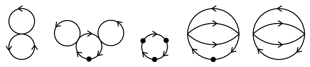
At the transition, the diagrams of Fig. 8 cancel at second order in $a$, as do the diagrams of Fig. 9, because of the first-order relation of Fig. 1. So we may simplify our task by focusing on just the diagrams of Fig. 7.

At this many loops, organizing all the terms of the matching calculation becomes tedious unless one from the start uses dimensional regularization for the IR (as well as the UV). In the 3-dimensional theory, the loop integrals in Fig. 7 then all vanish by dimensional analysis, leaving us with the formal result

$$-{\partial f\over\partial\mu}=-{\partial f_{3}\over\partial\mu}$$

(49)

for dimensionally regulated perturbation theory. In the 3+1 dimensional theory, we have

$$-\left({\partial f\over\partial\mu}\right)_{\mu_{\rm c}}=\hbox{$\sum$}\!\!\!\!\!\!\int_{P}{1\over(ip_{0}+\omega_{p})}+(\mu_{\rm c}-\mu_{\rm c}^{[1]})\hbox{$\sum$}\!\!\!\!\!\!\int_{P}{1\over(ip_{0}+\omega_{p})^{2}}+\delta n_{\rm bball}+{\cal O}(a^{3})$$

(50)

at the transition, where

$$\mu_{\rm c}^{[1]}={8\pi a\over m}\hbox{$\sum$}\!\!\!\!\!\!\int_{P}{1\over(ip_{0}+\omega_{p})}$$

(51)

is the first-order result for $\mu_{\rm c}$, determined by Fig. 1, and

$$\delta n_{\rm bball}\equiv{1\over 2}\left(-{8\pi a\over m}\right)^{2}\hbox{$\sum$}\!\!\!\!\!\!\int_{PQK}{1\over(ip_{0}+\omega_{p})^{2}(iq_{0}+\omega_{q})(ik_{0}+\omega_{k})(i(p_{0}+q_{0}+k_{0})+\omega_{{\bf p}+{\bf q}+{\bf k}})}$$

(52)

is the contribution of the last diagram of Fig. 7, which we refer to as the basketball diagram.³³ 3 Historical note: The origin of this terminology in the literature is associated with the physical appearance of old American Basketball Association basketballs, not current National Basketball Association ones. In section V, we will show how to evaluate this integral in dimensional regularization, with the result that

$$\delta n_{\rm bball}={32\pi a^{2}\over\lambda^{5}}\left[{\sqrt{\pi}\over 2}-K_{2}+(2K_{1}+\ln 2)\,\zeta({\textstyle{1\over 2}})-{\ln 2\over 2\sqrt{\pi}}\,\left[\zeta({\textstyle{1\over 2}})\right]^{2}\right]+{\cal O}(\epsilon),$$

(53)

where $K_{1}$ and $K_{2}$ are numerical constants defined by⁴⁴ 4 For efficient numerical evaluation of $K_{1}$, it’s useful to make a change of integration variables in (54), such as $u=\sqrt{1-t}$, which makes the integrand analytic at both endpoints.

	$\displaystyle K_{1}$	$\displaystyle\equiv$	$\displaystyle{1\over 4\pi}\int_{0}^{1}{dt\over t}\>\left[\left[{\rm Li}_{1/2}(t)\right]^{2}-{\pi t\over 1-t}\right]\simeq-0.630~568~207~496~069,$		(54)
	$\displaystyle K_{2}$	$\displaystyle\equiv$	$\displaystyle{1\over 4\pi}\int_{0}^{1}{ds\over s}\>{dt\over t}\biggl\{{\rm Li}_{1/2}(s)\,{\rm Li}_{1/2}(t)\,{\rm Li}_{-1/2}(st)$		(55)
			$\displaystyle\hskip 40.00006pt-{st\sqrt{\pi}\over 2(1-st)^{3/2}}\left[\sqrt{\pi\over 1-s}+\zeta({\textstyle{1\over 2}})\right]\left[\sqrt{\pi\over 1-t}+\zeta({\textstyle{1\over 2}})\right]\biggr\}$
		$\displaystyle\simeq$	$\displaystyle-0.135~083~353~73.$

${\rm Li}_{\nu}(z)$ is the polylogarithm function defined by

$${\rm Li}_{\nu}(z)=\sum_{n=1}^{\infty}{z^{n}\over n^{\nu}}.$$

(56)

[The polylogarithm function is often called $g_{\nu}(z)$ in statistical mechanics.]

The other integrals in the matching (50) are given by (40) and

$$\hbox{$\sum$}\!\!\!\!\!\!\int_{P}{1\over ip_{0}+\omega_{p}}=M^{\epsilon}\lambda^{-d}\,\zeta\left({\textstyle{d\over 2}}\right),$$

(57)

which is discussed in Appendix A. Putting it all together and taking $d\to 3$,

$$-\left({\partial f_{3}\over\partial\mu}\right)_{\mu_{\rm c}}=\zeta({\textstyle{3\over 2}})\,\lambda^{-3}+\zeta({\textstyle{1\over 2}})\,\lambda^{-3}\,(\beta\mu_{\rm c}-\beta\mu_{\rm c}^{[1]})+\delta n_{\rm bball}+{\cal O}(a^{3})\,.$$

(58)

In Ref. [6], a second-order matching calculation was carried out for $\mu_{3}$ that determined $\mu_{\rm c}$ in terms of the critical value of $r$ in the 3 dimensional theory. The result was

$$\beta\mu_{\rm c}=\beta\mu_{\rm c}^{[1]}+{32\pi a^{2}\over\lambda^{2}}\left[\ln(\bar{M}\lambda)+C_{1}-72\pi^{2}\,{r_{\rm c}(\bar{M})\over u^{2}}\right],$$

(59)

with $C_{1}$ a numerical constant that was given in that reference in terms of a somewhat inelegant double integral. In section VI, we show that $C_{1}$ can also be expressed as

$$C_{1}={\textstyle{1\over 2}}-{\textstyle{1\over 2}}\ln(32\pi)-2K_{1}.$$

(60)

Combining the last several formulas, and choosing $\bar{M}=u/3$ to make contact with the quoted lattice measurement (25b) of $r_{\rm c}$, we have

	$\displaystyle-\left({\partial f_{3}\over\partial\mu}\right)_{\mu_{\rm c}}$	$\displaystyle=$	$\displaystyle\zeta({\textstyle{3\over 2}})\,\lambda^{-3}+{32\pi a^{2}\over\lambda^{5}}\biggl\{\left[\ln\left(a\over\lambda\right)+{\textstyle{1\over 2}}\ln(128\pi^{3})+{\textstyle{1\over 2}}-72\pi^{2}{\cal R}\right]\zeta({\textstyle{1\over 2}})$		(61)
			$\displaystyle\hskip 80.00012pt+{\sqrt{\pi}\over 2}-K_{2}-{\ln 2\over 2\sqrt{\pi}}\left[\zeta({\textstyle{1\over 2}})\right]^{2}\biggr\}+O\left(a^{3}\over\lambda^{6}\right).$