Energy Spectrum of a Relativistic Two-dimensional
Hydrogen-like Atom in a Constant
Magnetic Field of arbitrary strength
Víctor M. Villalba11 1 e-mail: villalba@ivic.ve, Ramiro Pino22 2 e-mail: rpino@win.ue.nl
11 1 e-mail: villalba@ivic.veCentro de Física, Instituto Venezolano de Investigaciones Científicas, IVIC
Apdo 21827, Caracas 1020-A, Venezuela
Department of Mathematics and Computing Science
Technische
Universiteit Eindhoven,
P. O. Box 513 Eindhoven 5600 MB, The Netherlands
We compute, via a variational mixed-base method, the energy spectrum of a two dimensional relativistic atom in the presence of a constant magnetic field of arbitrary strength. The results are compared to those obtained in the non-relativistic and spinless case. We find that the relativistic spectrum does not present states.
PACS 31.20. -d, 32.60. +i, 03.65. Ge
1 Introduction
Two-dimensional Hydrogen atoms in magnetic fields have been a subject of active research during the last years. A large body of articles has been published on this problem in the framework of non-relativistic quantum mechanics. This problem is of practical interest because of the technological advances in nanofabrication technology that have made possible to create low dimensional structures like quantum wells, quantum wires and quantum dots [1, 2, 3]. The two-dimensional Hamiltonian describing the Coulomb interaction , between a conduction electron and donor impurity center when a constant magnetic field is applied perpendicular to the plane of motion, can be written in atomic units, in the CGS system, as follows
| (1) |
Since we are dealing with a two-dimensional problem, we choose to work in polar coordinates The angular operator operator commutes with the Hamiltonian (1), consequently we can introduce the following ansatz for the eigenfunction
| (2) |
Substituting (2) into (1), we readily obtain that the radial function satisfies the second order differential equation
| (3) |
where is the Larmor frequency, is the energy, and the eigenvalue of the angular momentum. Eq. (3) cannot be solved in closed form in terms of special functions [4]. There are analytic expressions for the energy for particular values of and [5, 6, 7]. The computation of the energy eigenvalues in (3) has been carried out using different techniques [8, 9, 10, 11, 12, 13]. A less studied problem is that of a relativistic 2D hydrogen atom in a magnetic field. Perhaps relativistic effects are not very important in semi-conducting devices but nevertheless they cannot be neglected when the interacting potentials are strong [14, 15]. Recently, the importance of considering relativistic effects has been pointed out when one computes the energy levels of semiconductors in high magnetic fields[16]. The effective mass method is still valid until Oe. In the case of two band approximation, the dispersion law has the form of a Klein-Gordon energy spectrum[17]. Also, relativistic invariance imposes some supplementary restrictions on the allowed quantum energy levels.
In this article we investigate the relativistic corrections to the energy spectrum of a two-dimensional hydrogen atom in an homogeneous transverse magnetic field. Using a mixed-basis variational approach [18, 19]. In Sec 2, we compute the relativistic energy spectrum of a 2D relativistic Klein-Gordon hydrogen atom. In Sec 3, we discuss the application of the expansion to our problem. In Sec 4, we compare the energy spectrum of the relativistic 2D hydrogen atom with that obtained in the nonrelativistic limit. Finally, we present the concluding remarks in Sec. 5.
2 Relativistic Hydrogen Atom
Since we are interested in discussing the relativistic corrections to the energy levels of the 2D Hydrogen atom, we proceed to solve the 2D Klein-Gordon equation. The results obtained after solving the Klein-Gordon equation apply to an electron without spin. The advantage of this approach [15] can be easily understood if we recall that the Schödinger equation does not take into account the spin of the electron (1) and then we can directly compare the relativistic and nonrelativistic energy spectra.
The covariant generalization of the Klein-Gordon equation in the presence of electromagnetic interactions takes the form [13, 20]
| (4) |
where is the contravariant metric tensor, and is the covariant derivative. The metric tensor written in polar coordinates takes the form:
| (5) |
and the vector potential associated with a 2D Coulomb potential and a constant magnetic field interaction is
| (6) |
From the above expression (6) for the vector potential it is straightforward to verify that the electric and magnetic fields satisfy the invariant relations
| (7) |
| (8) |
where is the (2+1) electromagnetic field strength tensor.
Expressions (7) and (8) tell us that in fact, is associated with a 2D Coulomb atom in a constant magnetic field perpendicular to the plane of the particle motion. The corresponding and can be written in polar coordinates as follows:
| (9) |
Since the vector potential components do not depend on time or the angular variable we have that the wave function , solution of the Klein-Gordon equation (4), can be written as
| (10) |
where the function satisfies the second order differential equation
| (11) |
Eq. (11) has the same form as Eq. (3), therefore no exact solutions of Eq. (11) can be obtained in terms of special functions.
In the present article we analyze the problem of computing the energy levels of the 2D relativistic Coulomb atom using a mixed-basis variational approach. In order to apply the variational method to our problem [20], we look for a trial wave function. Since Eq. (11) reduces to the relativistic Hydrogen atom equation when we can consider as a basis, for , the Hydrogen wave functions The solution of eq. (3) when is
| (12) |
where is a normalization constant, are the Laguerre polynomials [21], and from [22] is
| (13) |
It is worth mentioning that the relation (13) makes sense only when
| (14) |
a condition that forbids the existence of the energy levels (, this is in fact a peculiarity of the relativistic Klein-Gordon solution, which is not present in the standard Schrödinger framework.
Conversely, for large values of a good trial basis is that of the spherical oscillator. In this case, the solution of eq. (11) has the form
| (15) |
and, in the high-field limit, the energy spectrum of a relativistic spinless particle in a constant magnetic field satisfies the relation
| (16) |
Among the advantages of considering a relativistic spinless electron is that we can easily compute the energy levels with the help of the mixed base variational approach. Nevertheless, we can easily see when the Klein Gordon equation gives a reasonably good value for the energy spectrum as compared to that obtained via the Dirac equation.
The 2+1 Dirac equation [27, 28] in the presence of an external electromagnetic field reads
| (17) |
Since we are working in a two dimensional space, we can work in the following representation of the gamma matrices
| (18) |
Then, the Dirac spinor has only two components. Since the Dirac equation (17) expressed in the diagonal tetrad gauge commutes with the operators and , the spinor can be written as
| (19) |
| (20) |
where and satisfy the system of equations
| (21) |
| (22) |
Substituting (21) into (22), we obtain the following second order differential equation
| (23) |
where is given by
| (24) |
It is worth mentioning that angular parameter takes half integer values [27] and therefore it can be related to as follows
| (25) |
Eq. (23) reduces to the radial Klein-Gordon equation (11) when vanishes. Looking at (24) and (21) we see that is very small for large values of [28]. The mean square radius of the Dirac and Klein-Gordon electron is where labels the energy levels. Taking into account that large values of the radial variable imply that , we find that is negligible for magnetic fields satisfying the inequality , which is the critical value for strong magnetic fields [29].
Using Eq. (23), and keeping only leading terms of , the motion of a relativistic electron for small values of and is described by the equation
| (26) |
Notice that Eq (26) gives a description of a relativistic electron in a weak magnetic field for small values of . From Eq. (23) and (25, we see that, in oposition to the Klein-Gordon case, the 2+1 relativistic Dirac electron has states.
If we attempt to apply the variational method using the hydrogen atom basis, we will obtain good agreement with accurate results for small values of but this approach fails for large , even if we consider a many term basis. An analogous situation occurs when we use the oscillator basis, in which case we obtain a good agreement for large but the convergence is very slow for small values of . [23] In order to solve this problem, we propose a trial function [18, 19], for any quantum level , a linear combination of the form
| (27) |
where ; and are the corresponding hydrogen and oscillator wave functions associated with the quantum level and are constants to be calculated. It is worth mentioning that our basis is not orthogonal under the inner product Substituting (27) into (11), and performing variation on the basis coefficients , we readily obtain the following matrix equation:
| (28) | |||
with
| (29) |
where the indices i and j running from 1 to N correspond to the Hydrogen and oscillator bases respectively. The algebraic equation (28) gives nontrivial values of provided that the matrix be singular. The energy eigenvalue for a given quantum level is the lowest value of solution of the equation The mixed-basis variational method gives reasonably good values for the energy eigenvalues even for the simple selection of a two term basis as in Eq. (27). In this particular case, we have that the trial function, for any quantum level, is a linear combination of the form
| (30) |
Better results should be expected for a basis with more terms. For a three term basis, we have two possible trial functions
| (31) |
and
| (32) |
where the three terms in (31) and (32) have the same angular dependences of the eigenfunction to be approximated. In this scheme u2i corresponds to a wavefunction associated with a higher quantum number to that we are going to approximate.
For comparison, the numerical computations of the relativistic energy spectra are carried out with the help of the Schwartz method [24], which is a generalization of the mesh point technique for numerical approximation of functions. This method gives highly accurate results given a thoughtful choice of the reference function, and its efficiency has been shown computing the energy spectrum of the 2D Hydrogen atom [13].
3 1/N Approach
The shifted 1/N expansion is a perturbative technique that has permitted us to solve the N-dimensional stationary Schrödinger equation with a wide class of radial potentials. The shifted 1/N method has also been developed to compute energy eigenvalues of relativistic spin 0 and spin particles in the presence of spherically symmetric vector and scalar potentials. Here we proceed to compute the energy eigenvalues of our problem using the 1/N expansion for . Since Eq. (11) contains a magnetic field contribution, some minor modifications should be made to the recipe of Ref [25] where the authors develop the shifted 1/N technique to deal with the Klein-Gordon equation in a spherically symmetric potential.
Following the scheme developed by Imbo and Pagnamenta [10], we have that the radial Klein-Gordon equation in the presence of a constant magnetic field (9) takes the form
| (33) |
where with as the shifting parameter, and is the reduced radial wave function. Eq. (33) is written in units . In these units we have that . Here we borrow the results reported in Ref [25] Introducing the scaled mass
| (34) |
and proceeding to minimize
| (35) |
we obtain that satisfies the equation
| (36) |
The shifting parameter is
| (37) |
where is given by
| (38) |
and can be written as
| (39) |
with
| (40) |
Equations (37) and (39) along with equations (38) and (40) give
| (41) |
Equation (41) allows computing the value of Using this value we compute the coefficients
| (42) |
| (43) |
| (44) |
| (45) |
and finally we have for the energy
| (46) | |||
where the energy level is expressed in units where The energy eigenvalues can be expressed in atomic units with the help of the relation:
| (47) |
Now we proceed to compare the results obtained via the mixed variational approach as well as the expansion with those computed numerically. Energy levels are computed in Rydberg units as a function of and displayed in Figures 1 to 4.

.


.

4 Comparison with the 2D nonrelativistic Hydrogen Atom
In this section we proceed to compare the results obtained for the energy spectrum of the 2D relativistic Hydrogen atom with those computed in the nonrelativistic limit, when the 2D Schrödinger equation was considered. In order to establish a better comparison we use numerical results obtained with the Schwartz interpolation method[24]. In Tables 1 and 2 we exhibit different values of the energy for different magnetic field strengths.
| nonrel | rel | diff x 100 | |
|---|---|---|---|
| 0 | -0.4444444 | -0.44449574 | 0.005134 |
| 0.1 | -0.5239504 | -0.52421206 | 0.026166 |
| 0.2 | -0.5629132 | -0.5635173 | 0.06041 |
| 0.3 | -0.5635941 | -0.56468762 | 0.109352 |
| 0.4 | -0.5193465 | -0.52115542 | 0.180892 |
| 0.5 | -0.4095808 | -0.41248102 | 0.290022 |
| 0.6 | -0.1862031 | -0.19088784 | 0.468474 |
| 0.7 | 0.2719562 | 0.2640041 | 0.79521 |
| 0.8 | 1.3504374 | 1.33516298 | 1.527442 |
| 0.9 | 5.1012487 | 5.0599714 | 4.12773 |
Table 1 Relativistic energy values for , and a comparison with the non relativistic energy spectrum. The first column corresponds to the nonrelativistic energy, the second column is the relativistic energy , and the third column corresponds to 100 times the difference between first and second columns
| nonrel | rel | diff x 100 | |
|---|---|---|---|
| 0 | -0.16 | -0.1600366 | 0.00366 |
| 0.1 | -0.2605089 | -0.2606836 | 0.01747 |
| 0.2 | -0.2731927 | -0.27364026 | 0.044756 |
| 0.3 | -0.2377636 | -0.2386137 | 0.08501 |
| 0.4 | -0.150434 | -0.1518818 | 0.14478 |
| 0.5 | 0.0113883 | 0.00901904 | 0.236926 |
| 0.6 | 0.3009099 | 0.29702154 | 0.388836 |
| 0.7 | 0.8503051 | 0.84361474 | 0.669036 |
| 0.8 | 2.0734797 | 2.06046406 | 1.301564 |
| 0.9 | 6.1341553 | 6.09847572 | 3.567958 |
Table 2 Relativistic energy values for , and a comparison with the non relativistic energy spectrum. The fist column corresponds to the nonrelativistic energy, the second column is the relativistic energy, and the third column corresponds to 100 times the difference between first and second columns
Tables 1 and 2 show that the role played by the relativistic corrections is to shift down the energy levels. The relativistic effects becomes noticeable when the magnetic field parameter is close to unity. Figure 5. shows the dependence of this difference.
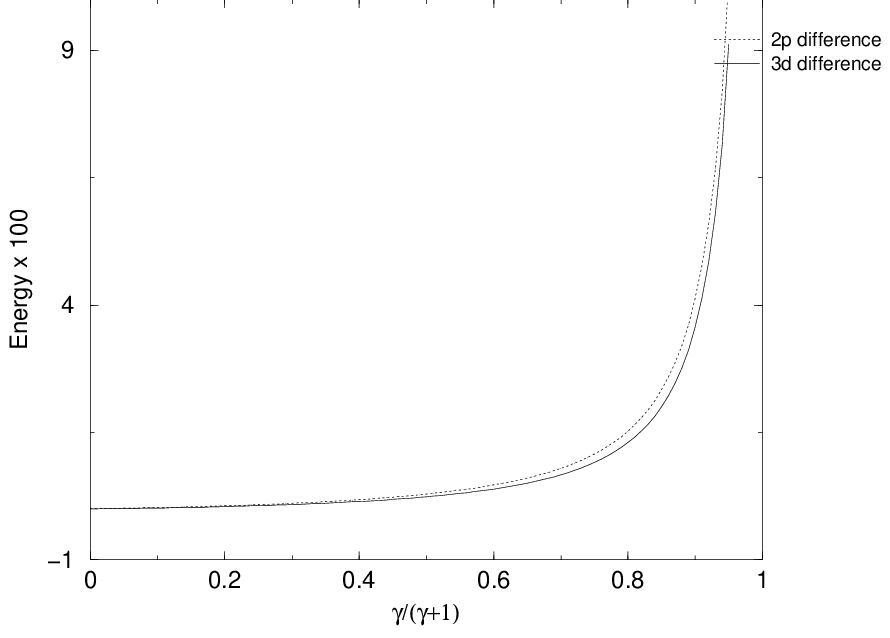
.
5 Concluding remarks
Figures 1 thru 4 show that the variational mixed-basis method gives very good results for the energy spectrum of a 2D relativistic Hydrogen atom in a constant magnetic field. The energy eigenfunctions obtained with this approach give good energy values even for intermediate values of as shown in Figs 1-4 where we compare the variational results with those obtained numerically via the Schwartz interpolation method [24]. The shifted method fails to give reasonably results when we apply its extension to the Klein Gordon equation [25]. The advantage of the mixed variational method is that we obtain a simple form of the wave function and a reasonable good approximation without considering a large term variational basis. The role played by relativity consists in shifting down the energy levels as indicated in Figure 5. The results presented in this article were obtained considering a two-dimensional hydrogenic atom in the presence of a magnetic field perpendicular to the plane of motion. In this direction there are some differences between our approach and the method applied in Ref. [18, 19]. Here the authors consider a non relativistic quasi two-dimensional system confined by a square-well . The Hamiltonian in Ref. [18, 19] contains this term and therefore the energy spectrum depends on the dimensions of the confining well. Since the variational technique applied in this paper is equivalent to the method suggested by Chen et al [18, 19], our results reduce, in the non relativisic limit, and when the width of the well is negligible, to those reported by Chen et al. Finally we mention that states are not present for the 2D Klein-Gordon Hydrogen atom. The absence of states for the relativistic Klein-Gordon 2D Hydrogen atom can be understood if we look at the behavior of Eq. (11) as approaches to zero. For m=0, we have a “falling to center” problem[26], and this behavior is unobserved when we solve the 2D Dirac equation. A detailed discussion of relativistic effects including spin corrections will be presented in a future publication.
Acknowledgments
We thank Dr. Ernesto Medina for reading and improving the manuscript. This work was supported by CONICIT under project 96000061.
References
- [1] R. L Greene, and K. K. Bajaj Phys. Rev. B 31 (1985) 913.
- [2] N. F. Johnson J. Phys.: Condens. Matter 7 (1995) 965
- [3] T. Chakraborty Comments Cond Mat. Phys. 16 (1992) 35.
- [4] V. G. Bagrov and D. M. Gitman Exact solutions of relativistic wave equations Dordretch: Kluwer. 1990.
- [5] E. D. Lozanskii, O. B. Firsov 1974 Izv. Vyssh. Ucheb. Zav. Fizika. 6 (1974) 52.
- [6] M Taut J. Phys. A: Math. Gen. 28 (1995) 2081
- [7] M Taut Phys. Rev A. 48 (1993) 3561
- [8] A. H. MacDonald and D. S. Ritchie. Phys Rev B. 33 (1986) 8336.
- [9] P Martín, J. J. Rodríguez and J. L. Márquez Phys.Rev. B. 45 (1992) 8359.
- [10] T. Imbo, A. Pagnamenta, and U. Sukhatme Phys. Rev. D. 29, (1984) 1669.
- [11] O. Mustafa J. Phys : Condens. Matter 5, (1993) 1327.
- [12] O. Mustafa J. Phys: Condens. Matter 8, (1996) 8673.
- [13] V. M Villalba, and R. Pino J. Phys: Condens. Matter 8, (1996) 8667.
- [14] R. J. Elliot, and R. Loudon J. Phys. Chem. Solids 15, (1960)196.
- [15] H. N. Spector and J. Lee Am. J. Phys 53 (1985) 248.
- [16] A. A. Avetisyan, A. P. Djotyan, E. M. Kazaryan, and H. A. Sarkisyan Phys. Stat. Sol. (b) 214 (1999) 91.
- [17] L. V. Keldysh. Zh. Eksper. Teor. Fis. 45, (1963) 364.
- [18] R. Chen, J. P. Chen, D. L. Lin, and B. D. McCombe Phys. Rev B. 44 (1991) 8315.
- [19] R. Chen, J. P. Chen, D. L. Lin, B. D. McCombe, and T. F. George J. Phys: Condens. Mattter 7 (1995) 3577.
- [20] A. S. Davydov Quantum Mechanics Oxford: Pergamon. 1965.
- [21] N. N. Lebedev Special functions and their applications Dover, New York. 1972
- [22] M. M. Nieto Am. J. Phys 47 (1979) 1067.
- [23] V. M Villalba, and R. Pino Phys. Lett A 238 (1998) 49. (1998)
- [24] C Schwartz J. Math. Phys. 26, (1985) 411.
- [25] O. Mustafa, and R. Sever Phys. Rev A. 43 (1991) 5788.
- [26] L. D. Landau, and E. M. Lifshitz Quantum Mechanics Pergamon, London, 1978
- [27] G. V. Shishkin, and V. M. Villalba J. Math. Phys. 30 (1989) 2373.
- [28] V. R. Khalilov Theor. Math. Phys. 119 (1999) 481.
- [29] V. R. Khalilov Electrons in strong magnetic fields Energoatomizdat, Moscow 1988.