[
Extensive eigenvalues in spin-spin correlations: a tool for counting pure states in Ising spin glasses
Abstract
We study the nature of the broken ergodicity in the low temperature phase of Ising spin glass systems, using as a diagnostic tool the spectrum of eigenvalues of the spin-spin correlation function. We show that multiple extensive eigenvalues of the correlation matrix occur if and only if there is replica symmetry breaking. We support our arguments with Exchange Monte-Carlo results for the infinite-range problem. Here we find multiple extensive eigenvalues in the RSB phase for , but only a single extensive eigenvalue for phases with long-range order but no RSB. Numerical results for the short range model in four spatial dimensions, for , are consistent with the presence of a single extensive eigenvalue, with the subdominant eigenvalue behaving in agreement with expectations derived from the droplet model. Because of the small system sizes we cannot exclude the possibility of replica symmetry breaking with finite size corrections in this regime.
]
I Introduction
In three spatial dimensions or higher it is now accepted that Ising spin systems with random exchange interactions, exhibiting disorder and frustration, undergo a transition from a paramagnetic phase to a glass phase at a finite temperature. [1] By contrast, the nature of the glass phase at finite dimensions is still a subject of much debate in the literature, with two main competing points of view. One follows Parisi’s solution of the Sherrington-Kirkpatrick (SK) model [2] using a replica symmetry breaking (RSB) ansatz. [3] The Parisi solution involves broken ergodicity of a subtler form than that found in a conventional ferromagnet: configuration space is broken into many ergodic regions, separated by energy barriers which diverge in the thermodynamic limit. Most of these regions—which we will also call pure states—are unrelated to one another by any symmetry of the Hamiltonian. However, in the case of a Hamiltonian with global spin inversion symmetry, each of these regions has an associated region related to it by global spin inversion, the pair forming together what we will call a pure state pair (PSP). This RSB picture is almost certainly correct in the limit of infinite spatial dimension; and it has been argued that the RSB picture also applies, more or less unchanged, to the frozen phase of finite-dimensional spin glasses. The other point of view is the ‘droplet’ picture, [4] which, in sharp contrast to the picture just described, postulates the presence of a single PSP in the low-temperature phase. In this paper we focus on the fundamental difference between these two pictures, namely, the nature of the ergodicity breaking in spin glasses—or, put more simply, the number of ‘valleys’ (ergodic regions) in the low-temperature phase.
The glass transition is characterized by the Edwards-Anderson spin-glass order parameter
| (1) |
which becomes nonzero [i.e., of ] for . Here is the spin at site , is the number of spins in the system, indicates an average over disorder realizations and indicates a thermal average. The order parameter may also be obtained as the first moment of the overlap distribution function
| (2) |
where , label pure states, indicates the overlap between the local magnetizations in two pure states, and is the thermodynamic weight of pure state . In the thermodynamic limit, is predicted to have very different behaviors in the two pictures mentioned above. For a single PSP, approaches a pair of delta functions at , where is the self-overlap of each pure state in the pair, and is the overlap between one pure state and the other. For the diverging (countable) number of PSPs in the SK problem is nonzero over a finite interval (this property depends essentially on the fact that is a disorder averaged quantity). So far, the main tool for detecting non-trivial broken ergodicity in finite dimension at nonzero temperatures has been the scaling of the overlap distribution function at as a function of system size: for a single PSP it must scale to zero, while it remains nonzero in the thermodynamic limit if there is RSB. Several numerical studies have suggested a behavior in finite dimensions similar to the one at the mean field level. [5, 6] Other studies using the Migdal-Kadanoff approximation, [7] and still others investigating the ground state susceptibility to boundary conditions [8] have suggested otherwise and favor the droplet model. None of these studies has conclusively resolved which type of broken ergodicity takes place in the low temperature phase in finite dimensions, motivating a search for new approaches.
In this paper we propose and apply a rather direct method for determining the number of PSPs for an Ising spin glass. Our main ideas were introduced in a previous Letter; [9] here we provide an extended development of these ideas, along with further analytical and numerical results. Our method involves the study of the spectral properties of the spin-spin correlation function . It is inspired by Yang’s analysis [10] of correlation functions to detect off-diagonal long-range order (ODLRO) in superfluids. In the case of superfluids, Yang showed that the existence of ODLRO is equivalent to the presence of an extensive eigenvalue in the spectrum of the one-particle density matrix. We argue that, in the case of classical spin glasses, the spectrum of the spin-spin correlation function contains a distinct signature which allows one to determine unambiguously whether or not there are many pure state pairs, i.e. whether or not RSB occurs. First of all, it is clear that the presence of at least one extensive eigenvalue signals the presence of long-range order. What we further show is that the number of extensive eigenvalues determines unambiguously the number of pure state pairs: the spectrum contains exactly one extensive eigenvalue if and only if there is exactly one pure state pair, and it contains more than one extensive eigenvalues if and only if there are more than one pure state pairs. We also argue that the extensive eigenvalues dominate the trace of , and that the nonextensive eigenvalues scale with the number of spins in the system with a power lower than . We confirm these arguments by performing Exchange Monte Carlo [6, 12] (EMC) simulations for the SK model in various regimes, for which we know the nature of the ergodicity breaking in the equilibrium state. That is, we find multiple extensive eigenvalues in the spin-glass phase, but only a single such eigenvalue in the ferromagnetic phase and in the paramagnetic phase in a field. In the RSB phase (where one expects many PSPs) we find that, for the range of system sizes that we have studied, the eigenvalue spectrum is dominated by a small number of extensive eigenvalues. Making the simplifying assumption that the thermal average is dominated by only two PSPs, we are able to introduce an analytically calculable model which reproduces the eigenvalue spectrum for the SK model surprisingly well. Finally, we use EMC simulations to study the Edwards-Anderson (near-neighbor) model in four spatial dimensions. Our results, for system sizes , are compatible with the presence of only one extensive eigenvalue of . The second largest eigenvalue of is very well fit (with ) by a power-law scaling with , with an exponent (smaller than one) that is consistent with the value predicted by the droplet theory. An alternative fit with a form that allows for an extensive piece in the second largest eigenvalue of is possible [11], although it would imply that the ratio of the eigenvalue over saturates to a finite value, something that is not observed in our data.
We organize this paper as follows. In Sec. II we show how the properties of the spectrum of below can be used to distinguish between RSB and a single PSP in the low temperature phase. In Sec. III we discuss numerical results for the SK model in its various regimes. In Sec. IV we introduce a two-PSP model and show that it gives results much like the numerical results for the SK model. In Sec. V we present and discuss the results of our EMC simulations for the short-range Edwards-Anderson model in four dimensions. Finally, in Sec. VI we present our conclusions.
II Spin-spin correlators and pure states in Ising systems
Guided by the analogy to Yang’s analysis of the matrix elements of the one particle density matrix in a superfluid system, we study the spectrum of the spin-spin correlation matrix of an Ising spin system. This matrix has an extensive trace . In addition, it is positive semi-definite: for an arbitrary real N-dimensional vector ,
Above the ordering temperature decays exponentially to zero at large , so it has no large eigenvalues. For (or for in the SK model, for which distance is not meaningful), the correlation matrix reduces to the identity , and consequently all its eigenvalues are equal to one. Below , however, is nonzero almost everywhere due to the ordering of the spins. For one PSP, in the low temperature limit , , has one eigenvalue which approaches as , and the rest of the eigenvalues go to zero. Hence, there is a transition in the distribution of the eigenvalues of as crosses . Specifically, just as in the case of superfluids and ferromagnets and antiferromagnets, we can detect the existence of long range order below by the presence of one (or more) extensive eigenvalue(s). This approach based on examining the spectrum of the correlation functions has a definite advantage in the study of disordered systems: we can eliminate the necessity for guessing the nature of the order—i.e., the eigenvectors corresponding to the extensive eigenvalues—and still detect its existence. We will also find that this spectrum can give unique and clear information about the number of pure states in a frozen, disordered phase.
Although the spin-spin correlation function has not been extensively used to probe the nature of the broken ergodicity in the spin glass phase, many related quantities have been used to study some of the static properties of spin glasses. For example, the quantity
| (3) |
is a commonly used order parameter in spin-glass systems. [1] Also, the spin-glass susceptibility for one disorder realization (i.e. for a fixed set of spin couplings )
| (4) |
is given, for , by
| (5) |
We see that the disorder average of contains interesting information about the freezing of the spins (while in contrast the disorder average of contains no information—it is just the unit matrix). For , becomes of order , the largest eigenvalue of becomes of order , and becomes of order . Hence our measure of order () is consistent with earlier measures used for spin glasses.
We wish further to obtain new and independent information from the spectrum of ; towards this goal, in the following two subsections we will argue that one can detect the presence or absence of order with many valleys (i.e., RSB) simply by counting the number of extensive eigenvalues of . To make this connection, the main idea used will be that pure states are characterized by their clustering [13] property, i.e. that the spin-spin correlation function at long distances can be approximately decomposed as a linear combination of (possibly non-orthogonal) projectors onto the subspaces associated with the pure states present in the system, i.e.:
| (6) |
where denotes a thermal average restricted to the pure state . From this relation, a connection will be obtained between the number of extensive eigenvalues of the left hand side and the number of pure state pairs present in the right hand side. The rest of this section is devoted to deriving this connection, and to estimating the effects on the spectrum due to the terms neglected in Eq. (6).
II.1 Single pure state pair
We first consider the case of a single PSP. We show that in this case there is only one extensive eigenvalue that dominates the trace of .
Without loss of generality, we can consider the case of only one pure state. This applies directly if one of the pure states in the pair is selected by an external field or a boundary condition. But even when the two pure states are present, the spin-spin correlation matrix for the system is the same as if only one of them was present, simply because it involves a product of an even number of spin variables. [14]
Hence we can rewrite as
| (7) | |||||
| (8) | |||||
| (9) |
where is the connected correlation function. By arguments similar to the one used to show that is positive semi-definite, both and are positive semi-definite (see Appendix A).
Let’s ignore for the moment the connected part , and concentrate on the matrix . This matrix is proportional to the projector onto the vector , thus it has exactly one extensive eigenvalue
| (10) |
(where is the self-overlap of the pure state) with eigenvector proportional to , and eigenvectors with eigenvalue zero.
We then ask how the matrix changes this distribution of eigenvalues. By the clustering property of pure states [13], the typical element of vanishes as ; hence it is reasonable to assume that the typical value of the ratio between the largest eigenvalue of and the largest eigenvalue of goes to zero in the thermodynamic limit. By a detailed variational argument (see Appendix B), it can be shown that the largest eigenvalue of is bounded between and , and in the case that the second largest eigenvalue of is bounded above by times a number that goes to one. In other words, the largest eigenvalue of the correlation matrix remains extensive (and, in fact, it changes very little) when the effect of is included. This result can also be recovered more intuitively by applying perturbation theory to the problem of estimating the effect of .
The problem that remains to be solved is, therefore, the estimation of the largest eigenvalue of . A possible assumption would be that the off-diagonal parts of have a typical behavior in the large- limit of , with . (The diagonal elements are always , but they have an effect of order on the eigenvalues.) The largest eigenvalue of , and therefore the second largest eigenvalue of , are then of order . One can also view this result in the following way. can at most reweight the eigenvalues of as if it is an additional pure state with thermodynamic weight (see Sec. IV), in which case it gives rise to an eigenvalue (again) . An eigenvalue of order is, in principle, distinguishable from an eigenvalue of order , since .
In some cases it is possible to obtain a stronger bound on the decay exponent . For instance, if we assume that , then we get by simple power counting. This should be the case everywhere above the Almeida-Thouless (AT) line [15] in the phase diagram [16] for the SK model. Above this line there is a paramagnetic phase with a single pure state, with long-range order trivially induced when the external magnetic field is nonzero. There is also a conventional ferromagnetic phase with a single PSP, in another part of the phase diagram but still above the AT instability. Either of these phases should have decaying with . For a pure ferromagnet with no frustration or disorder, assuming (as appropriate for a single PSP) the uniform susceptibility is of gives the stronger constraint . We expect this latter limit to be approached for the SK problem, when either the external magnetic field or the average ferromagnetic coupling are sufficiently large.
While the above arguments make no direct reference to spatial dimension, they do rely on the notion of a ‘typical’ element of . This idea is certainly appropriate for infinite-range models such as the SK problem; and the above arguments may also be applied to any finite-dimensional problem for which a typical behavior of can be defined. For example, one can define a typical for any magnetic system with a finite correlation length; here the typical is exponentially small and so the matrix does not have significant effects on the eigenvalues of . However, correlations in finite-dimensional spin glasses, in the frozen phase, are thought to fall off more slowly than exponentially, [18] giving an infinite spin-glass susceptibility in the spin-glass phase [4, 17] and rendering the notion of a typical element of problematic.
Hence we examine carefully the ‘droplet’ theory, [4] which is the outstanding candidate for a theory of finite-dimensional spin glasses without RSB. In this theory the low energy excitations at large distances are assumed to be large droplets of collectively overturned spins of size , whose energy scales as . It follows that the majority of the elements of are exponentially small; however there is also a set of ‘big’ elements which are of in magnitude. These elements occur when and lie within the same ‘active’ (coherently flipping) droplet; this makes and small, while leaving and large. The fraction of these big elements is of order , where is the system size and is a scaling exponent from the zero-temperature fixed point. Although this ‘big’ fraction vanishes in the thermodynamic limit, it still can have large effects at large . For example, let us suppose that a finite sample of size is dominated by one large active droplet of size of order . In such a case the big elements of , appearing with probability , are coherent, so that the largest eigenvalue of is of order . (We have verified this with simple numerical experiments.) Given this bound on the eigenvalues of , the largest eigenvalue of is again much smaller than the largest eigenvalue of , and again the second largest eigenvalue of is of order or smaller. Hence one gets a decay exponent for equal to . Given the assumptions leading to this conclusion, this value is a lower bound for the rate of decay of . It is plausible however that, for a range of system size not too large, the assumption of dominance by a single active droplet can hold, giving this lower bound for . Furthermore, the numerical value of the latter can be quite small: about in three dimensions, [19] and about in four. [20] Hence one needs good numerical data for in a finite-dimensional spin glass to distinguish RSB (with ) from a which is weakly decaying due to droplet excitations.
II.2 Many pure state pairs
In the previous subsection we have presented strong arguments, assuming there is only a single PSP in the low temperature phase, that there can be only one extensive eigenvalue of . It follows from our argument that the observation of more than one extensive eigenvalue directly implies RSB. In short, letting be the number of PSPs, and be the number of extensive eigenvalues, we found
| (11) |
or
| (12) |
Now we would like to argue that the converse is also valid, i.e., to find some necessary consequence of RSB in the eigenvalue spectrum. Hence we will assume RSB (that there is more than one pure state pair present), and then determine how many extensive eigenvalues there should be in the spectrum of the spin-spin correlation matrix.
Let us suppose that there are pure states, characterized by the magnetizations (), and thermodynamic weights , with . Here we only include pure states whose thermodynamic weight is nonvanishing. We now decompose the correlation function into the contributions coming from each pure state:
| (13) | |||||
| (14) |
with
| (15) | |||||
| (16) | |||||
| (17) |
By the clustering property of pure states, we may assume that is small compared with . As in the case of one PSP, we will proceed in two steps. First we will study the spectrum of , and later we will include the effect of .
Let’s define the vectors
| (18) |
with the coefficients to be determined later. For an appropriate choice of the , these vectors can be shown to be eigenvectors of . In fact,
| (19) | |||||
where we have defined the real, symmetric matrix . The matrix has orthonormal eigenvectors with eigenvalues . By inserting one of these eigenvectors in Eq. (18) we obtain
| (20) |
Thus, for each nonzero eigenvalue of , an eigenvector of is obtained with eigenvalue . Let’s denote by the number of linearly independent magnetization vectors among the magnetizations of the pure states (). This number need not be equal to : for example, the magnetizations of the two pure states in a PSP are not linearly independent, since one of them is times the other. Having is equivalent to saying that there is either only one pure state present, or there is exactly one PSP. Therefore, for the droplet picture and for the RSB picture strictly, i.e.:
| (21) |
It is an exercise in linear algebra to show that (see Appendix A): (i) the number of nonzero eigenvalues of is exactly , (ii) all of these nonzero eigenvalues are positive, (iii) the corresponding eigenvectors of are linearly independent, and (iv) the remaining linearly independent eigenvectors of have zero eigenvalue and are orthogonal to all pure state magnetizations. As a consequence, the number of nonzero extensive eigenvalues of is equal to , the number of pure states with linearly independent magnetizations.
Next we assess the effects of . We assume that the sum over pure states is finite (see below, and Ref. 26). Hence, even if the decay at different rates with , we can still take the typical element of to decay with at least as fast as for some . Hence the largest eigenvalue of is of order or smaller. From this we can show (Appendix B) that there are still extensive eigenvalues for ,
| (22) |
Combining this with Eq. (21) it follows that
| (23) |
It is plausible, although not proven, that in general a complete set of pure states not related by spin inversion (thus constituting one-half of the total set of pure states) will all be, with probability one, linearly independent, so that is just the number of PSPs, i.e. .
Note that, in the Parisi RSB solution [13] to the mean-field problem, the number of PSPs grows with , at a rate which is not known. The ultrametric structure of these pure states implies [21] that they cannot grow in number faster than . However there is a stronger constraint, coming from Eq. (47) of Ref. 26, which states that . This tells us that the diverging number of pure states do not have equal thermodynamic weight; instead a finite number of them dominate the sum of the weights , with the rest having negligible weight.
One might ask whether the ultrametric structure of the space of pure states might imply some constraint on the number which are linearly independent. However we find no such constraint in general. For example, one can construct, for any number (where is the dimension of the vector space), a set of vectors which are both linearly independent and ultrametric; but one can also construct a set which is linearly dependent and ultrametric.
It may be possible to derive tighter bounds on these quantities via further theoretical work. In the following section we provide some further information, obtained from equilibrium Monte-Carlo studies, on for a finite range of in the SK problem.
III Results for the SK model
The SK model is described by the Hamiltonian
| (24) |
with and for any and . This model, which is equivalent to an infinite dimensional model for which mean field theory is exact, has a phase diagram [16] in (,,) space which is reasonably well understood. In particular, there are instability lines (which presumably form a surface) below which the replica symmetric solution is unstable, and the Parisi RSB ansatz [3] is believed to give the correct solution. The ‘AT line’ found by de Almeida and Thouless [15] lies in the - plane (i.e., ); below this AT line there is RSB, while increasing either or brings one to a phase consisting of a single pure state. This phase is continuous with the paramagnetic phase at ; it has long-range order which is trivially induced by the field, and hence neither spontaneous symmetry breaking nor broken ergodicity of any other sort. Nevertheless we expect a large eigenvalue for due to the long-range order. In another region of parameter space (, with a ferromagnetic bias sufficiently large) there is a ferromagnetic phase with one PSP. Here one has the familiar version of broken ergodicity in the form of spontaneous symmetry breaking; given that there is a single PSP, we expect a single extensive eigenvalue in this phase also. Thus we find three distinct phases (glass/RSB, paramagnet+field, ferromagnet) which we can explore via Monte Carlo simulations in order to test our ideas about correlation functions, eigenvalue counting, and ergodicity breaking in Ising systems.
We have performed EMC [12, 6] simulations for the SK model at three points in the phase diagram. In glassy systems with very long relaxation times, normal Monte Carlo simulations are limited to small system sizes because of the divergent relaxation and equilibration times. [25] EMC simulations allow for the crossing of barriers in a reasonable simulation time, via a stochastic walk of each simulated system not only in configuration space but also in temperature. The simulation consists of having many systems at different temperatures for the same disorder realization running in unison, and attempting to exchange the configurations between adjacent temperatures after a given number of Monte Carlo steps . The exchange of neighboring temperature configurations takes place with the probability
| (25) |
with
| (26) |
and indicating the instantaneous spin configuration at temperature . With this probability of exchange one ensures that the systems at the different temperatures remain in thermal equilibrium—whether or not they exchange temperatures—at all times during the simulation. This is because the configuration obtained from an exchange with a higher temperature is still accepted with the normal Boltzmann probability for the lower (accepting) temperature; hence an exchange drives neither system out of equilibrium. If the temperature difference between neighboring systems is not too large, then exchanges are accepted at a reasonable rate, and each system explores the full range of temperatures. Hence each system is effectively cooled and heated many times during the simulation, ensuring that all barriers have been effectively circumvented, not by crossing them but by falling within their boundaries from a higher temperature. An important parameter in this simulation is the spacing between the different temperatures, which must be adjusted to get a high enough acceptance ratio for the temperature exchanges. [6, 12]
Our criteria for having reached thermal equilibrium in our measured quantities involve calculating the spin-glass susceptibility for a single disorder realization using two distinct methods. One method, discussed extensively in previous studies, [24] uses the averaging of the overlap of two uncoupled replicas
| (27) |
and the other uses the standard way of calculating the thermal average in Monte Carlo simulations.
| (28) |
Here and have to be chosen large enough to obtain thermally equilibrated results. We also demand full symmetry of the overlap distribution function , and that all initial configurations visit all temperatures evenly. We have also checked our results using commonly studied quantities such as and doing standard Monte Carlo simulations for the smaller system sizes; here our results are in agreement with previous work. [24, 25] In our simulations we have used a temperature spacing of , , , and . (Here all times are in units of Monte Carlo steps per spin.)
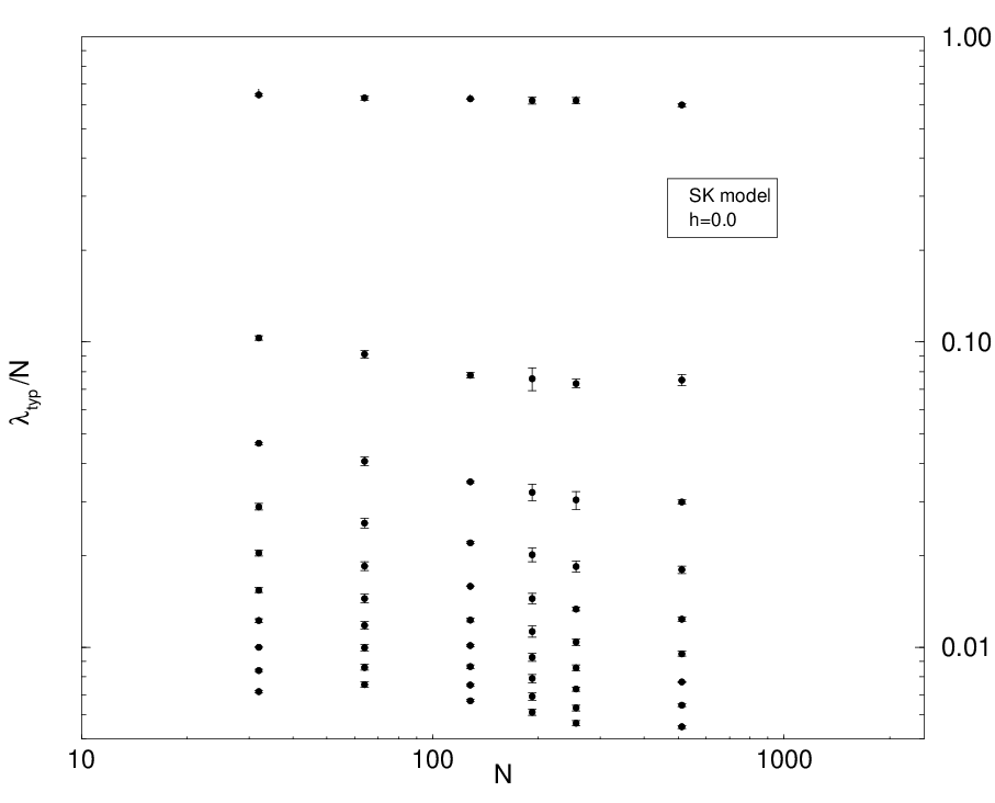
We find that the eigenvalue spectrum of is strongly dependent on disorder realization, such that it is impossible to observe any regular dependence of the on with increasing for a single set of ’s. (See Fig. 6 below for examples of similar behavior in four space dimensions.) Hence it is necessary to accumulate statistics on the eigenvalue spectra for many disorder realizations. The eigenvalue probability distribution for the first two eigenvalues of for at zero field and at (above the AT line)—all at —are shown in Fig. 1. These distributions have been obtained from 3400 disorder realizations. It is clear from Fig. 1 that, at least in the RSB phase, the distributions for and are extremely broad; also they show significant skew. Hence we have studied both and for small in each phase.
We show the average of the ten largest eigenvalues as a function of system size in Fig. 2 for different points of the SK phase diagram: (a) , , , the RSB phase; (b) , , , the paramagnet in field with one pure state; and (c) , , , the ferromagnet with a single PSP. The system sizes considered are and with and disorder realizations performed respectively. It is clear from Fig. 2(a) that two eigenvalues are of order for . This is extremely strong [23] numerical evidence for more than one PSP, and hence nontrivial ergodicity breaking. We expect further eigenvalues to emerge for larger , as suggested by the behavior of in the figure.
In contrast, there is only one large eigenvalue in Fig. 2(b) and (c). We find further that may be fit to a power law for some range of in cases (b) and (c). In the paramagnetic phase (b) while in the ferromagnet (c) is somewhat larger, . While we do not expect these power laws to have reached their asymptotic values for the system sizes considered here, we do expect any observed decay for large enough to be consistent with our arguments in the previous section, where we obtained in this regime. MC results for the paramagnetic phase, in a larger field than in (b), show that decays with a larger exponent (we have observed up to ), which we expect to approach 1 for large enough . We also show in Fig. 3 the scaling of the typical value for the first ten eigenvalues in the RSB phase. Here the behavior is qualitatively similar to that of in Fig. 2(a): both figures show clearly that (av or typ) is flat as a function of above a threshold value for which is of order 100–200, plus strong signs that and are also approaching a flat behavior. Hence we see graphically, in these figures, the emergence of multiple PSPs with increasing .
Figs. 2 and 3, taken together, give convincing evidence that the eigenvalue spectrum of can clearly distinguish trivial (one PSP) from nontrivial broken ergodicity. This spectrum allows one, for large enough , to detect multiple PSPs simply by counting the number of extensive eigenvalues . As discussed above, while the number of PSPs is believed to diverge in the thermodynamic limit, only a few of them dominate the thermodynamics; [26] we see some of these emerging in Figs. 2(a) and 3. A possible consequence of this would be that, for large enough , might saturate at a finite constant. The present data show no clear sign of this, although they are clearly beyond the threshold of for which begins to exceed . For in the vicinity of this threshold, we expect that one can reasonably view the glass phase as having just two PSPs; and we explore the consequences of this assumption next.
IV Two pure state pairs
As suggested by Figs. 1, 2, and 3, the spectrum of for the SK problem is dominated by two large eigenvalues, each coming from a broad distribution of values, for the system sizes considered here. We can understand much of this behavior with a simple two-PSP model which can be computed analytically. We begin with a very simple model for two PSPs at . Suppose that phase space consists of only two spin configurations 1 and 2, and ignore all others. Take , with and corresponding to the of the two different configurations and at zero temperature, and (a thermodynamic weight) ranging from 0 to 1/2. The overlap between the two states is given by . It can be easily shown that this matrix has only two nonzero eigenvalues, corresponding to
| (29) |
Note that ranges from at to at . It is also clear that, for small , is linear in ; hence if is of lower order in than , ceases to be extensive. At the same time, even if the two PSPs have equal thermodynamic weight, the second eigenvalue approaches zero as and as . This is consistent with our results from Section II, since as the two states become linearly dependent and becomes . We can proceed further with this two-PSP model by calculating the probability distribution of and , as follows:
| (30) |
where is the probability distribution of , depends on , and is an implicit function of given by . For the case of this simplifies to
| (31) |
and
| (32) |
here . At this simple level of approximation we already have the first indication that the probability distribution of the first and second eigenvalues will be very broad in the case of non-trivial broken ergodicity—as we have seen in the MC results. Note however that in spite of the breadth of the distribution are still proportional to . Let us now augment this picture with finite-temperature effects. An approximate way to introduce temperature into the two-PSP model is as follows. We let
| (33) |
where and are gaussian random variables with the mean of equal to . We adjust the distribution of and such that agrees with that obtained from our MC runs, while also demanding that the overlap distribution agree with —which can also be extracted from our MC , by subtracting a Gaussian part due to the self-overlap . The result of this decomposition procedure is illustrated in Fig. 4. This gives us a means of generating a realistic sample of matrices corresponding to two PSPs. We can then obtain the first few eigenvalues of and compare them with the eigenvalues obtained directly from the MC simulations of the SK model. The former eigenvalues may be obtained either by an approximate analytical perturbation approach (using only the diagonal part of ), or by direct numerical diagonalization of the matrix —which must in any event be generated by a random number generator. Fig. 5 shows the eigenvalue distributions obtained from our two-PSP model with , compared with those obtained directly from the EMC runs, for the SK model in the glass phase at . It is encouraging that our simple picture of two PSPs, with a minimal set of assumptions, reproduces both the position and the shape of the two distributions.
We believe—and Fig. 5 supports this belief—that the assumption of two PSPs has validity for a range of near the threshold where RSB first appears. We also believe that this assumption will fail for larger ; our Monte-Carlo results strongly suggest that the number of significant PSPs will exceed two as grows. It is interesting to ask what the large- limit of is. We obtain no answer to this question from the considerations of Section II; while our numerical results suggest only that is at least as large as 3 or 4. We note here that Fig. 5 itself may be viewed as giving some indication of a third large eigenvalue, if we assume (as is plausible from our two-PSP results) that the third PSP robs weight from the upper part of .
V Results for the EA model in four dimensions
We have performed EMC studies of the four-dimensional Ising spin glass on a hypercubic lattice, with nearest-neighbor interactions, periodic boundary conditions, and a gaussian distribution of the ’s with zero mean. The parameters of the calculation follow closely those of Ref. 6. We have focused on the point and . These simulations are rather deep in the frozen phase, since . We choose this low temperature in order to try to avoid spurious effects from closeness to the critical region; such effects are likely to make it difficult to distinguish multiple PSPs from a single PSP. The price we pay is that our MC runs are slow to converge, while—according to the estimates of Ref. 18—we are still not fully out of the critical region. Our criteria for convergence are the same here as those we used for the SK model (Sec. III).
We have only examined the frozen phase for this problem. We find that a plot of the distributions for and gives broad and skewed forms similar to those seen for the RSB phase in Fig. 1. To complement the picture given in Fig. 1, we show in Fig. 6 some examples of the typical behavior of a single disorder realization at “fixed” ’s and increasing . Here “fixed” is in quotation marks since (as is well known for spin glasses) adding spins requires adding bonds, and hence a change in the , which can often have nontrivial effects. Fig. 6 bears out this expectation: the eigenvalue spectrum of shows a highly irregular behavior as a function of . If this irregularity were to persist in the limit (such that the eigenvalues, and hence the correlations, had no well-defined limit), then according to Newman and Stein, [27] there must be more than a single pure-state pair. That is, “chaotic size dependence” is believed to characterize glasses with RSB, but not to occur for a single PSP (unlike chaotic temperature dependence [28]). While the behavior shown in Fig. 6 is interesting in this regard, we do not believe any conclusion can be drawn from these data due to the small size of the systems considered here. Instead we will focus on trying to count extensive eigenvalues—a strategy that worked well for the SK problem. Fig. 6 suggests rather strongly that is extensive; but it is impossible to draw any conclusion about , and so we again resort to disorder averaging.
In Fig. 7 we show (a) and (b) for the first ten eigenvalues of , at and . The system sizes shown in Fig. 7 are , , , and with , , , and disorder realizations respectively. These data suggest that and are each decaying with , with a clean power law . A fit of the data in Fig. 7 gives (a) for the average eigenvalues, and (b) for the typical eigenvalues, . The exponent we find for is close to that expected from our argument of Section II.1, coupled with previous estimates for the exponent . The latter range [29, 12] from 0.6 to 0.8, while a simple extrapolation [20] suggests . Our own argument () predicts a minimum value for in the range 0.15 to 0.2; hence the behavior of is roughly consistent with this prediction, while for is somewhat smaller.
The decay of is quite regular. Moreover, there is rough agreement between the exponent obtained from the typical eigenvalues and the exponent estimated by assuming the droplet picture to be valid. This evidence seems to favor the scenario of only one PSP being present.
Of course, it is in general difficult to settle from numerical simulations alone any question that involves behaviors of a physical system in the thermodynamic limit, since the results observed for some sizes can change when larger sizes are simulated. In particular, any claim that RSB does not occur, based on our method, is necessarily more tentative than a conclusion that it does occur. [23] Thus the results we obtain for cannot rule out the possibility of further PSPs appearing at some larger , indicating that there is RSB in the spin-glass phase in four dimensions. By contrast, if the droplet picture is correct for 4D spin glasses, then we believe that the decay exponent should, for sufficiently large , increase from its lower bound as the dominance of a single droplet fails. Hence any sign of curvature of the log-log plot of vs. , in either direction, would be of significant interest.
It is also of interest to push results like those of Fig. 6 to larger . Here one seeks signs of convergence (or lack of it) to a limit. This criterion is, we believe, more difficult to assess than the criterion we have applied to Figs. 2, 3, and 7. The latter criterion has the nice property that one must only ascertain whether an integer—the number of extensive eigenvalues—is one, or greater than one. However studies seeking chaotic size dependence can certainly complement studies of disorder-averaged eigenvalue scaling.
VI Conclusions
In this work we have applied the old idea of studying the eigenvalue spectrum of a correlation function—used by Yang [10] to characterize ODLRO in superfluids—to a decades-old question in spin-glass physics, namely: how many pure states are there in the frozen phase, and how are they related? The connection we have made is simple: for problems in which the low-temperature phase has multiple pure states (of non-negligible thermodynamic weight) not related by spin inversion symmetry, the broken ergodicity shows up as multiple extensive eigenvalues of the spin-spin correlation matrix . We have strong arguments in two directions: first, that the presence of multiple extensive eigenvalues necessarily implies nontrivial ergodicity breaking, i.e., multiple pure-state pairs; and second, that the presence of multiple pure-state pairs will give rise to multiple extensive eigenvalues. We have found striking support for these arguments from numerical (Monte-Carlo) studies of the Sherrington-Kirkpatrick problem in three distinct phases—the paramagnetic, ferromagnetic, and replica-symmetry-broken (RSB) phases. Specifically, we find clear and unambiguous signs of the different kinds of ergodicity breaking in these three phases via studies of the dependence of the disorder-averaged eigenvalues of —which essentially enable us to count the number of extensive eigenvalues, and hence the number of pure-state pairs in the configuration space. We believe that the evidence for RSB displayed in Figs. 2(a) and 3 is unique in its directness, clarity and lack of ambiguity.
We have also applied these ideas to the near-neighbour Ising spin glass in four dimensions. Our data are consistent with the presence of only one extensive eigenvalue, for . Furthermore, the typical value of decays with a clean power law; and the exponent agrees roughly with the value expected from an argument based on the droplet picture, plus independent estimates of the scaling exponent . An alternative analysis that assumes that a second extensive eigenvalue is present with large finite size corrections cannot be completely excluded, although the lack of any restriction on the fitting parameters makes any conclusions drawn from such fits (in general of higher ) questionable. Thus our results tend to support the ‘droplet’ picture of the frozen phase, with a single PSP, more strongly than they support the RSB picture. We believe that studies of the kind reported here should be extended to larger in order to test this tentative conclusion. Our present results encourage us to believe that such studies can play an important role in settling the question, from the theoretical side, of the nature of the broken ergodicity in real spin glasses.
The authors acknowledge helpful discussions with J. Hu, E. Sorensen, and G. Parisi. This work was supported by the National Science Foundation under grants DMR-9820816 and DMR-9714055.
Appendix A Properties of the matrices , and
In this appendix we show that: (i) the symmetric matrices defined in Sec. II, , (both of size ) and (of size ), are positive semi-definite, (ii) the rank of is equal to (the number of pure states with linearly independent magnetizations), (iii) the eigenvectors of constructed via Eq. (18) from the linearly independent eigenvectors of with positive eigenvalue are linearly independent, and (iv) the remaining linearly independent eigenvectors of have zero eigenvalue and are orthogonal to all pure state magnetizations.
We start by showing that is positive semi-definite: for an arbitrary real N-dimensional vector ,
| (34) | |||||
Similarly, in the case of we have,
| (35) | |||||
We now concentrate in studying the matrix . By convention, we enumerate the pure states so that the first magnetization vectors are linearly independent. Now, for any real -dimensional vectors and we have,
| (36) | |||||
By choosing we immediately see that is positive semi-definite. Thus statement (i) is proven.
We will now study the eigenvectors of the matrix . Consider Eq. (36) in the case that and is chosen such that
| (37) |
Since by our assumptions are linearly independent and are nonzero, we have that
| (38) |
By the Gram-Schmidt procedure, we can obtain normalised vectors that are orthogonal with respect to , all satisfying (37). This means that
| (39) |
where the are positive numbers. The will be shown below to be eigenvectors of with eigenvalues , but first it is necessary to construct the eigenvectors with zero eigenvalue. To do that, let us consider the magnetization vectors with , that can be written as linear combinations of the first ones (i.e. the ones that are linearly independent):
| (40) |
This allows to construct the linearly independent vectors , of the form
| (41) |
which satisfy
| (42) |
by Eq. (40). Combining this with Eq. (36) it follows that for an arbitrary dimensional real vector
| (43) |
This means that all of the are eigenvectors of with zero eigenvalue. By the Gram-Schmidt procedure, an orthonormal set of linear combinations of them can be constructed. By combining Eq. (39) and Eq. (43) we get:
| (44) | |||||
and therefore statement (ii) is proven.
Consider now the vectors of the form proposed in Eq. (18) associated with the eigenvectors of with positive eigenvalue. Since the matrix () is invertible, and the magnetization vectors ) are linearly independent, it follows that the vectors are linearly independent. Thus statement (iii) is proven.
The remaining eigenvectors of can be constructed as follows. Take an arbitrary vector in the -dimensional subspace orthogonal to the magnetization vectors (and consequently orthogonal to all of the magnetization vectors of the pure states). Clearly, is a null vector for since
| (48) |
and this proves statement (iv).
Appendix B Spectrum of
In this appendix some bounds are shown to be satisfied by the changes in the eigenvalues of the spin-spin correlation matrix due to the effect of .
For a given disorder realization, temperature and size , let us consider the eigenvalues and eigenvectors of the correlation matrices and :
| (49) |
where the eigenvalues are positive and labeled in descending order (the subscript corresponding to the highest eigenvalue for each matrix). We label by the largest eigenvalue of the matrix . We will use variational arguments to show that:
- •
For any value of ,
(50) - •
For , and if the ratio is small enough, then:
(51)
Let’s consider Eq. (50) first. The upper bound is obvious once is decomposed as a sum of and , and use is made of the fact that any mean value for each one of them has to be smaller or equal than their respective maximum eigenvalues:
| (52) |
To prove the lower bound in the case , we just consider the eigenvector corresponding to the largest eigenvalue of , and use it as a variational trial vector:
| (53) |
where we have used the fact that is positive semi-definite.
To prove the lower bound for general , we use an inductive reasoning. We assume that Eq. (50) is valid for all , and propose as a variational trial vector a linear combination of . Because it is generated by linearly independent vectors, this linear combination can be chosen to be orthogonal to all of the exact eigenvectors . Then we have
| (54) |
where we have used the facts that i) the term corresponding to has as a lower bound, and ii) is positive semi-definite. This proves the inductive step, and therefore Eq. (50).
Let’s consider the inequality Eq. (51). To prove it, we decompose the eigenvector into a part proportional to and a part orthogonal to it:
| (55) |
where is a normalised vector orthogonal to . We now write the matrix elements of in the subspace generated by and :
| (56) |
The coefficient that parametrizes Eq. (55) can be related to these matrix elements by
| (57) |
and therefore satisfies the bound
| (58) |
We now consider the eigenvector , corresponding to , the second largest eigenvalue of . Since is normalized and orthogonal to , it has the form:
| (59) |
where is a normalized vector orthogonal both to and to . From the expression for :
| (60) | |||||
we immediately obtain the bound:
| (61) |
From Eq. (58), it is clear that for we have:
| (62) | |||||
References
- [1] K. Binder and A. P. Young, Rev. Mod. Phys. 58, 801 (1986).
- [2] D. Sherrington and S. Kirkpatrick, Phys. Rev. Lett. 35, 1792 (1975).
- [3] G. Parisi, Phys. Rev. Lett. 43, 1754 (1979); J. Phys. A13, 1101 (1980); J. Phys. A13, 1887 (1980).
- [4] D. S. Fisher and D. A. Huse, Phys. Rev. Lett. 56, 1601 (1986); J. Phys. A 20, L1005 (1988); Phys. Rev. B 38, 386 (1988).
- [5] A. P. Young, Phys. Rev. Lett. 51, 1206 (1983).
- [6] E. Marinari and F. Zuliani, cond-matt/9904303.
- [7] M. A. Moore, Hemant Bokil, and Barbara Drossel, Phys. Rev. Lett. 81, 4252 (1998).
- [8] Matteo Palassini and A. P. Young, Phys. Rev. Lett. 83, 5126 (1999).
- [9] Jairo Sinova, Geoff Canright, and A. H. MacDonald, Phys. Rev. Lett. 85, 2609 (2000).
- [10] C. N. Yang, Rev. Mod. Phys. 34, 694 (1962).
- [11] In this case , which is still statistically acceptable, but a more important point is that given the small range of sizes several functional forms which would not correspond to a finite size correction also provide a similar fit.
- [12] K. Hukushima and K. Nemoto, cond-matt/9512035, K. Hukushima, cond-matt/9903391.
- [13] M. Mézard, G. Parisi, and M.A. Virasoro, Spin Glass Theory and Beyond (World Scientific, Singapore, 1987).
- [14]
To see this, first notice that (the superscripts and respectively label
quantities associated with one of the pure states and with the other,
spin reversed, one). Suppose that and are the
weights of the two pure states in the thermodynamic state of the
system; then
independently of the weights and . - [15] J.R.L. de Almeida and D.J. Thouless, J. Phys. A11, 983 (1978).
- [16] Fischer and Hertz (Ref. [17]), p. 80.
- [17] K.H. Fischer and J.A. Hertz, Spin Glasses (Cambridge University Press, Cambridge, 1991).
- [18] H. Bokil, B. Drossel, and M.A. Moore, Phys. Rev. B 62 946 (2000), cond-mat/0002130.
- [19] A.J. Bray and M.A. Moore, J. Phys. C 17, L463 (1984).
- [20] J.D. Reger, R.N. Bhatt, and A.P. Young, Phys. Rev. Lett. 64, 1859 (1990).
- [21] P. Baldi and E.B. Baum, Phys. Rev. Lett. 56, 1598 (1986).
- [22] A. P. Young, J. Appl. Phys. 57, 3361 (1985).
- [23] Given our arguments that the extensive eigenvalues count the pure state pairs, one need only assume that the leveling off of seen in Fig. 2(a) will not reverse itself with larger —a highly plausible assumption—in order to conclude, without the need for further study at larger , that RSB is occurring.
- [24] R. N. Bhatt and A. P. Young, Phys. Rev. B 37, 5606 (1988).
- [25] A. P. Young, J. Appl. Phys. 57, 3361 (1985).
- [26] M. Mézard, G. Parisi, N. Sourlas, G. Toulouse, and M. Virasoro, J. Physique 45, 843 (1984).
- [27] C.M. Newman and D.L. Stein, Phys. Rev. B 46, 973 (1992).
- [28] A.J. Bray and M.A. Moore, Phys. Rev. Lett. 58, 57(1987); J.R. Banavar and A.J. Bray, Phys. Rev. B 35, 8888 (1987).
- [29] A.K. Hartmann, Phys. Rev. E 60, 5135 (1999).