Current induced switching of magnetic domains to a perpendicular configuration

A system made of stacks of alternating ferromagnetic and non-magnetic metal layers shows Giant Magneto-Resistance (GMR) [1]: When two consecutive magnetic layers have their magnetic moments aligned, the conductance is much bigger than when they are anti-aligned. A simple way to think about this effect is in term of two separate (i.e., incoherent) currents for the majority and minority electrons (electrons with spin parallel or antiparallel to the magnetic moment, respectively), and to view the ferromagnetic layers as spin filters that have different conductances for majority and minority electrons [2]. In the configuration where the magnetic moments are aligned, the majority electrons are well transmitted by both magnetic layers while the minority electrons are (mostly) reflected. When the moments are anti-aligned, the majority spin direction of one layer is the minority spin direction of its neighbor so that all the electrons are reflected. The role of the magnetic field is to align the initially anti-aligned magnetic moments, thus giving rise to an increase of the conductance.

When the magnetic moments of the layers make an angle $\theta$ different from $0$ or $\pi$, the simple “two-current” picture does not hold anymore; instead a description in terms of a coherent superposition of spin up and spin down is needed. While the component of the spin flux in the direction of the magnetic moment $\vec{m}$ of a ferromagnetic layer is conserved when an electric current is passed through the layer (since the fluxes of majority and minority spins are conserved individually), the spin flux perpendicular to $\vec{m}$ does not have to be conserved, as it depends on the coherence between majority and minority electrons. As first pointed out by Slonczewski [3] and Berger [4], the consequence of such a change of the magnetic moment carried by the current is that the current exerts a torque on the moments of the ferromagnets. This so-called “spin-transfer” torque vanishes at the two angles $\theta=0$ and $\theta=\pi$, where the two current model applies. Experimentally, one studies a ferromagnet–normal-metal–ferromagnet (FNF) trilayer where one of the magnetic moments is held fixed, e.g. by using a thick ferromagnetic layer [5, 6, 7, 8], while the other one is free to rotate. The current direction determines which of the two angles $\theta=0$ and $\theta=\pi$ is stable; switching the current direction reverses the relative orientation of the magnets, and thus changes the conductance. This signature of the current-induced spin-transfer torque, which was observed experimentally in Refs [5, 6], provides a mechanism for a current controlled magnetic memory element. The spin-transfer torque can also be used for other applications  [9], including the excitation of spin-waves [10].

If one of the two external contacts of an FNF trilayer is replaced by a superconductor (S), see Fig. 1, the picture changes drastically. For voltages smaller than the superconducting gap, transport through the system occurs by Andreev reflection: an electron impinging on the S interface is reflected as a hole with opposite spin, adding a Cooper pair to the superconducting condensate. Each layer is therefore traversed twice, once by a majority electron (or hole) and once by a minority hole (or electron). Hence, the $\theta=0$ and $\theta=\pi$ configurations have the same conductance, the difference between them only being the order in which the spin filtering occurs[11].

What happens for angles $\theta$ other than $0$ or $\pi$? This question has a remarkable answer. While the presence of Andreev reflection suppresses the “usual” GMR at $\theta=0$ and $\pi$ (see previous paragraph), we have found that it leads to a richer variety of effects for other $\theta$, where quantum coherence between spin up and spin down is crucial. With the S contact, not only parallel or antiparallel alignment of the magnetic moments plays a special role, but also the perpendicular configuration: (1) As with normal contacts, passing a current through the FNFS system exerts a torque on the moments of the F layers; however, the possible stable configurations are not only $\theta=0$ and $\pi$, but also $\theta=\pi/2$ and $3\pi/2$. (2) The conductance $g$ is a $\pi$-periodic function of $\theta$ with a maximum for $\theta=\pi/2$. These two results were derived for the experimentally relevant case when the ferromagnetic moment $\vec{m}_{b}$ neighboring the superconductor is held fixed, while the other moment $\vec{m}_{a}$ is allowed to vary, see Fig. 1, and assuming that the spin-relaxation length is larger than the system size, which is a reasonable assumption for a thin trilayer system. By switching the current direction, one can switch the orientation of the free magnetic moment $\vec{m}_{a}$ from parallel to perpendicular to $\vec{m}_{b}$. Since $g(0)\neq g(\pi/2)$, such a switch can be observed through a change in the conductance, similar to what was observed in Refs. [5, 6] for the case of normal contacts. A magnetic field will align the moments, bringing the system from $\theta=\pi/2$ to $\theta=0$ (instead of $\theta=\pi$ to $\theta=0$), so that one should observe a positive magnetoresistance, in contrast to the standard GMR.

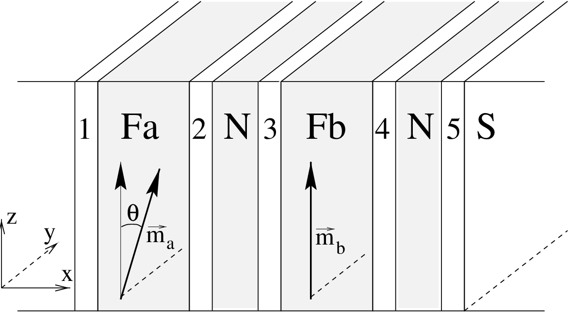
The FNF trilayer under consideration is shown in Fig. 1. The current flows in the $x$-direction, perpendicularly to the layers. For technical reasons, we have added thin ideal (non-magnetic) spacers labeled $1,\ldots,5$ between the F and N layers. Denoting the spin current in layer $i$ by $\vec{J}_{i}$ ($i=1,\ldots,5$), the torques $\vec{\tau}_{b}$ and $\vec{\tau}_{a}$ on the magnetic moments $\vec{m}_{a}$ and $\vec{m}_{b}$ are given by

$$\vec{\tau}_{b}=\vec{J}_{2}-\vec{J}_{4},\ \ \vec{\tau}_{a}=\vec{J}_{1}-\vec{J}_{2}.$$

(1)

Equation (1) expresses that, unlike the probability current, the spin current $\vec{J}$ is not conserved by the ferromagnetic layers. (The component of $\vec{J}$ in the direction of the magnetization is conserved, though.) The difference in spin currents is transfered to the F layers, as a torque acting on their magnetic moments.

We first give an intuitive explanation of how the presence of the superconductor allows for the additional stable configurations at $\theta=\pi/2$ and $\theta=3\pi/2$, and then present the results of a more rigorous calculation. For the intuitive explanation we make the simplifying assumption that spins scattered from an F layer with moment $\vec{m}$ have their magnetic moment pointing parallel (or antiparallel) to $\vec{m}$. (This assumption is valid if majority and minority electrons are transmitted incoherently; It is not necessary for the stability of $\theta=\pi/2$ or $3\pi/2$, as shown in our calculations below.) With this assumption, the explanation proceeds as follows (see right panel of Fig 2). (i) For voltages below the superconducting gap, only Cooper pairs can enter S. Hence, no spin current can flow into S and one must have $\vec{J}_{4}=\vec{J}_{5}=0$. Therefore, by Eq. (1), $\vec{\tau}_{b}=\vec{J}_{3}$. (ii) Since the spin flux in the direction of $\vec{m}_{b}$ is conserved, there can be no component of the torque $\vec{\tau}_{b}$ directed along $\vec{m}_{b}$. Hence $\vec{J}_{2}=\vec{J}_{3}$ is perpendicular to $\vec{m}_{b}$. (iii) Finally, for an unpolarized electron current entering the trilayer, any spin current in layer $1$ must be carried by electrons scattered from ${\rm F_{a}}$, so that $\vec{J}_{1}$ is parallel to $\vec{m}_{a}$. The torque $\vec{\tau}_{a}$ is then given by the component of $\vec{J}_{2}$ perpendicular to $\vec{m}_{a}$. Hence,

$$|\vec{\tau}_{a}|=|\vec{\tau}_{b}||\cos\theta|$$

(2)

$\vec{\tau}_{a}$ thus vanishes at $\theta=\pi/2$ and $3\pi/2$ yielding the new possibility of stable configurations at these angles.

To make the above picture more precise, we use the scattering approach [14, 15]. The trilayer is bounded in the $y$ and $z$ directions, so that its transverse degrees of freedom are quantized, giving $N_{\rm ch}$ propagating modes (“channels”) at the Fermi level. One has $N_{\rm ch}\sim A/\lambda_{F}^{2}$, $A$ being the cross section of the system and $\lambda_{F}$ the Fermi wave length. Expanding the electronic wave function in these modes, we can describe the system in terms of the $2N_{\rm ch}$-component vectors $\Psi_{i}^{e(h)L(R)}$, which is the projection of the wave function onto the left (right) going modes in region $i$ for the the electrons (holes) ($i=1,\ldots,5$). The $2N_{\rm ch}$ components of $\Psi$ account for the spin and channel degrees of freedom. In the scattering approach, each layer is characterized by $2N_{\rm ch}\times 2N_{\rm ch}$ reflection matrices $r_{i}$ and $r_{i}^{\prime}$ and transmission matrices $t^{\prime}_{i}$, $t_{i}$ (the label $i=1$ for ${\rm F_{a}}$, $i=3$ for ${\rm F_{b}}$, and $i=2,4$ for the two normal spacers),

	$\displaystyle\Psi_{i+1}^{eR}$	$\displaystyle=$	$\displaystyle t_{i}\Psi_{i}^{eR}+r^{\prime}_{i}\Psi_{i+1}^{eL},\ \ \Psi_{i+1}^{hR}=t_{i}^{*}\Psi_{i}^{hR}+{r^{\prime}_{i}}^{*}\Psi_{i+1}^{hL},$
	$\displaystyle\Psi_{i}^{eL}$	$\displaystyle=$	$\displaystyle r_{i}\Psi_{i}^{eR}+t^{\prime}_{i}\Psi_{i+1}^{eL},\ \ \Psi_{i}^{hL}=r_{i}^{*}\Psi_{i}^{hR}+{t^{\prime}_{i}}^{*}\Psi_{i+1}^{hL}.$		(3)

At the NS interface electrons are reflected as holes,

$$\Psi_{5}^{eL}=\sigma_{y}\Psi_{5}^{hR},\ \ \Psi_{5}^{hL}=-\sigma_{y}\Psi_{5}^{eL}.$$

(4)

To find the electrical and spin currents $I$ and $\vec{J}_{i}$ for each layer $i$, we need to calculate the generalized $2N_{\rm ch}\times 2N_{\rm ch}$ scattering matrices $S_{i,L(R)}^{e(h)e(h)}$ that give the amplitudes of left (right) moving electrons (holes) in region $i$ in terms of the amplitudes of the incoming electron (hole) in the normal electrode (labeled with layer index $i=1$),

$$\Psi_{i}^{e(h)L(R)}=S_{i,L(R)}^{e(h)e(h)}\Psi_{1}^{e(h)L}.$$

(5)

Using Eq.(3), the matrices $S_{i,L(R)}^{e(h),e(h)}$ can be expressed in terms of $r_{i}$, $r^{\prime}_{i}$, $t^{\prime}_{i}$ and $t_{i}$. (This was done in Ref. 13 for an FNF trilayer with two normal-metal contacts.)

Following the derivation of the Landauer formula for the conductance [12], one can now calculate the electrical current $I$ [17] and the spin current $\vec{J}_{i}$ for an applied voltage $V$ across the system as

	$\displaystyle{\partial I\over\partial V}$	$\displaystyle=$	$\displaystyle g=\frac{2e^{2}}{h}{\rm Tr}\,S_{1,L}^{eh}S_{1,L}^{eh\dagger},$		(6)
	$\displaystyle\frac{\partial\vec{J_{i}}}{\partial V}$	$\displaystyle=$	$\displaystyle-\frac{e}{4\pi}{\rm Re}\,{\rm Tr}\,\left[\vec{\sigma}S_{iR}^{ee}S_{iR}^{ee\dagger}\right.$		(7)
			$\displaystyle\left.\mbox{}-\vec{\sigma}^{*}S_{iR}^{he}S_{iR}^{he\dagger}-\vec{\sigma}S_{iL}^{ee}S_{iL}^{ee\dagger}+\vec{\sigma}^{*}S_{iL}^{he}\Lambda_{iL}^{he\dagger}\right].$

where $\vec{\sigma}=(\sigma_{x},\sigma_{y},\sigma_{z})$ is the vector of Pauli matrices.

It is important to notice that the scattering matrices need to be calculated for each individual layer only separately; solution of Eqs. (3) – (5) then describes how the information from the individual layers is combined to give properties of the multilayer system. For the ferromagnetic layers, the precise form of the reflection and transmission matrices has to be determined from a microscopic model, see e.g. Ref. 16. For the normal metal spacers, we make use of the polar decomposition [14],

$\displaystyle\left(\begin{array}[]{cc}r_{i}&t^{\prime}_{i}\\ t_{i}&r^{\prime}_{i}\end{array}\right)=\openone_{2}\otimes\left(\begin{array}[]{cc}u_{i}\sqrt{1-T_{i}}u^{\prime}_{i}&iu_{i}\sqrt{T_{i}}v_{i}\\ iv^{\prime}_{i}\sqrt{T_{i}}u^{\prime}_{i}&v^{\prime}_{i}\sqrt{1-T_{i}}v_{i}\end{array}\right),$

where $i=2,4$, $\openone_{2}$ is the $2\times 2$ unit matrix in the spin grading, $u_{i}$ $u_{i}^{\prime}$, $v_{i}$, and $v_{i}^{\prime}$ are $N_{\rm ch}\times N_{\rm ch}$ unitary matrices, and $T_{i}$ is a diagonal matrix containing the eigenvalues of $t_{i}t_{i}^{\dagger}$ on the diagonal. We consider an ensemble of trilayers for which the metallic spacers are good diffusive metals (with different impurity configurations for different members of the ensemble), or for which the interfaces between the different material are rough, so that the disorder mixes the different transverse modes in an isotropic way. In that case one can describe the ensemble by taking the unitary matrices $u$, $u^{\prime}$, $v$, and $v^{\prime}$ uniformly distributed in the unitary group [14]. We calculate an average over the matrices $u$, $u^{\prime}$, $v$, and $v^{\prime}$ to find the ensemble average of $\partial I/\partial V$ and $\partial\vec{J}_{i}/\partial V$. Since, fluctuations are of relative size $1/N_{\rm ch}$, the average is sufficient to characterize a single sample when $N_{\rm ch}\gg 1$. [14] (In the experiments, typically $N_{\rm ch}\sim 10^{3}$.)

After the ensemble average, the results only depend on four parameters for each ferromagnetic layer, [13]

	$\displaystyle T_{i\uparrow}$	$\displaystyle=$	$\displaystyle N^{-1}_{\rm ch}\mbox{tr}\,t_{i\uparrow}t^{\dagger}_{i\uparrow},\ \ T_{i\downarrow}=N^{-1}_{\rm ch}\mbox{tr}\,t_{i\downarrow}t^{\dagger}_{i\uparrow},$
	$\displaystyle T_{i\uparrow\downarrow}$	$\displaystyle=$	$\displaystyle N_{\rm ch}^{-1}\mbox{tr}\,t_{i\uparrow}t_{i\downarrow}^{\dagger},\ \ R_{i\uparrow\downarrow}=N_{\rm ch}^{-1}\mbox{tr}\,r_{i\uparrow}r_{i\downarrow}^{\dagger},$		(13)

on the conductances of the normal spacers, and on the angle $\theta$. In Eq. (13), the arrows refer to the majority and minority spin directions. The coefficients $T_{\uparrow\downarrow}$ and $R_{\uparrow\downarrow}$ describe the coherence of transmission and/or reflection of minority and majority spins. (The quantity $N_{\rm ch}-N_{\rm ch}R_{\uparrow\downarrow}$ is known as the “mixing conductance” [18].) The assumption of “incoherent” transmission and reflection of majority and minority that we made in the intuitive argument above, amounts to setting $T_{\uparrow\downarrow}$ and $R_{\uparrow\downarrow}$ to zero. This is a fair assumption for $T_{\uparrow\downarrow}$, since majority and minority electrons pick up different and uncorrelated phase shifts upon transmission through the ferromagnets, but it does not have to be the case for $R_{\uparrow\downarrow}$ when the reflection at the interface is instantaneous. For “perfect” spin filters, where all minority spins are reflected and all majority spins are transmitted, $T_{\uparrow\downarrow}$ and $R_{\uparrow\downarrow}$ are both zero.

The resulting expressions for the conductance and the torques are rather lengthy, and will not be reported here. Nevertheless, they allow us to draw general conclusions about the direction and magnitude of the torques for arbitrary values of the system parameters. First, in agreement with the simple argument given above, we find that the torques $\vec{\tau}_{a}$ and $\vec{\tau}_{b}$ lie in the plane spanned by the moments $\vec{m}_{a}$ and $\vec{m}_{b}$ [i.e., parallel to $(\vec{m}_{a}\times\vec{m}_{b})\times\vec{m}_{a}$ and $(\vec{m}_{b}\times\vec{m}_{a})\times\vec{m}_{b}$ respectively]. Second, the magnitudes of the torques $\vec{\tau}_{a}$ and $\vec{\tau}_{b}$ are related as

$$|\vec{\tau}_{a}|=-\frac{1-{\rm Re}\ T_{a\uparrow\downarrow}-{\rm Re}\ R_{a\uparrow\downarrow}}{1-{\rm Re}\ R_{a\uparrow\downarrow}}|\vec{\tau}_{b}||\cos\theta|,$$

(14)

irrespective of the conductances of the normal layers. This equation replaces Eq.(2) in case of non vanishing $R_{a\uparrow\downarrow}$ and $T_{a\uparrow\downarrow}$. In Fig. 2, we have indicated the directions of $\vec{\tau}_{a}$ and $\tau_{b}$ for various relative orientations of $\vec{m}_{a}$ and $\vec{m}_{b}$ and for the two possible directions of the current.

In Fig. 3, the torques $\vec{\tau}_{a}$ and $\vec{\tau}_{b}$ and the conductance $g$ are shown versus $\theta$, for realistic choices of the scattering parameters of the Co/Cu/Co trilayer used in the experiment of Ref. 5, 6, as they can be obtained through ab-initio calculations, see Ref. [16]. The torque and conductance for normal contacts with the same scattering parameters are also shown for comparison. Note that the presence of the superconducting contact does not affect the order of magnitude of the torques, or the sensitivity of $g$ to $\theta$. Therefore the critical current necessary to switch the layers’ magnetic moments should be in the same range as for N contacts ($I_{\rm crit}\sim 10^{9}{\rm A/cm}^{-2}$ in the point contact geometry of Ref. 5 and $\sim 10^{7}{\rm A/cm}^{-2}$ for the pillar geometry of Ref. [6]). This would allow, at least for the pillar geometry, the use of bias voltages below the superconductor gap. The main difference from the case of normal metal contacts is the period of the $\theta$-dependence of $\vec{\tau}_{a}$ and $g$, which changes from $2\pi$ to $\pi$. The $\theta$-dependence of the torque $\vec{\tau}_{b}$ on the layer adjacent to S is similar to what is found for the case of two normal leads. Although Fig. 3 is for a special choice of the parameters, we have verified that these conclusions do not depend on the detailed choice of scattering parameters.

In the limit when the conductance $g_{N}$ of the normal spacer connecting $F_{a}$ and $F_{b}$ is small, and when the mixed transmission and reflection probabilities $T_{\uparrow\downarrow}$ and $R_{\uparrow\downarrow}$ are $\ll 1$, simple expressions can be obtained for the torque and the conductance,

	$\displaystyle\frac{\partial\tau_{a}}{\partial I}$	$\displaystyle=$	$\displaystyle-\cos\theta\frac{\partial\tau_{b}}{\partial I}=\frac{g_{N}h}{16e\pi}\left(\frac{1}{T_{a\uparrow}}-\frac{1}{T_{a\downarrow}}\right)\sin 2\theta,$
	$\displaystyle g(\theta)$	$\displaystyle=$	$\displaystyle g(0)+\frac{e^{2}g_{N}^{3}}{2hN_{\rm ch}^{2}}\left(\frac{1}{T_{a\uparrow}}-\frac{1}{T_{a\downarrow}}\right)^{2}\sin^{2}\theta.$		(15)

Note that, in this limit, $\vec{\tau}_{a}$, $\vec{\tau}_{b}$, and $g$ do not depend on the detailed properties of layer $b$ but only on the direction of its magnetic moment $\vec{m}_{b}$.

The predicted absence of a GMR in the usual sense [$g(\theta)$ is equal for $\theta=0$ and $\pi$] requires some clarification, as GMR has been observed in multilayers with superconducting contacts [19], in contrast to our predictions and those of Ref. 11. One possible reason for the observed GMR is spin relaxation between the ferromagnetic layers and between the ferromagnetic layer and the superconductor. Especially for multilayer systems, spin relaxation can not be neglected. Another cause can be that ferromagnets not only serve as spin filters, but they also cause scattering from minority electrons into majority electrons and vice versa [11]. Finally, for ballistic FNFS layers, quantum interference effects that are not considered here can be important, thus providing another mechanism for the conventional GMR [20]. In each of these cases, the conductance of the multilayer will be different for $\theta=0$ and $\theta=\pi$, although the underlying reasons for this GMR are more subtle than in the case of normal metal contacts.

To conclude, we would like to emphasize that the stability of the perpendicular configuration is an intriguing feature; for example, it allows for the construction of a nanomagnet resonator with a current and magnetic-field controlled frequency: when a current is passed through the system such that the torque $\vec{\tau}_{a}$ keeps the moment $\vec{m}_{a}$ in the plane perpendicular to $\vec{m}_{b}$, an applied magnetic field parallel to $\vec{m}_{b}$ will make $\vec{m}_{a}$ precess in its plane with a frequency controled by the magnetic field.

We thank P. Chalsani, A. A. Clerk, E. B. Myers, and D. C. Ralph for friendly and useful discussions. We also acknowledge the hospitality of the Lorentz Center of Leiden University, where this work was initiated.

References

- [1] For a review, see F. J. Himpsel, J. E. Ortega, G. J. Mankey and R. F. Willis Adv. in Phys. 47, 511 (1998).
- [2] T. Valet and A. Fert Phys. Rev. B. 48, 7099 (1993).
- [3] J. Slonczewski, J. Magn. Magn. Mater. 159, L1 (1996).
- [4] L. Berger, Phys. Rev. B 54, 9353 (1996).
- [5] E. B. Myers, D. C. Ralph, J. A Katine, R. N. Louie, and R. A. Buhrman , Science 285, 867 (1999).
- [6] J. A. Katine, F. J. Albert, R. A. Buhrman, E. B. Myers, and D. C. Ralph, Phys. Rev. Lett. 84, 3129 (2000).
- [7] J-E. Wegrowe, D. Kelly, Y. Jaccard, Ph. Guittienne, and J-Ph. Ansermet, Europhys. Lett. 45, 626 (1999).
- [8] J. Grollier, V. Cros, A. Hamzic, J. M. George, H. Jaffrès, A. Fert, G. Faini, J. Ben Youssel, and H. Le Gall, preprint.
- [9] J. Slonczewski, U.S. Patent #5, 695, 864, Dec. 9, 1997.
- [10] M. Tsoi, A. G. M. Jansen, J. Bass, W.-C. Chiang, M. Seck, V. Tsoi, and P. Wyder, Phys. Rev. Lett. 80, 4281 (1998); 81, 493 (1998) (E).
- [11] F. Taddei, S. Sanvito, J. H. Jefferson and C. J. Lambert, Phys. Rev. Lett. 82, 4938 (1999); V. I. Fal’ko, C. J. Lambert and A. F. Volkov, Phys. Rev B 60 15394 (1999).
- [12] See, e.g., A. D. Stone in Mesoscopic Quantum Physics, E. Akkermans, G. Montambaux, J.-L. Pichard, and J. Zinn-Justin, eds, (North Holland, Amsterdam, 1995).
- [13] X. Waintal, E. B. Myers, P. W. Brouwer, and D. C. Ralph Phys. Rev. B 62, 12317 (2000)
- [14] C.W.J. Beenakker, Rev. Mod. Phys. 69, 731 (1997).
- [15] M. J. M. de Jong and C. W. J. Beenakker, Phys. Rev. Lett. 74, 1657 (1995).
- [16] M. D. Stiles, J. Appl. Phys. 79, 5805 (1996); Phys. Rev. B. 54, 14679 (1996).
- [17] C. L. Lambert J. Phys. C 3, 6579 (1991); Y. Takane and H. Ebisawa, J. Phys. Soc. Japan 61, 2858 (1992).
- [18] A. Brataas, Y. V. Nazarov and G. E. W. Bauer, Phys. Rev. Lett. 84 2481 (2000).
- [19] W. P. Pratt, Jr., S.-F. Lee, J. M. Slaughter, R. Loloee, P. A. Schroeder and J. Bass, Phys. Rev. Lett. 66, 3060 (1991).
- [20] N. Ryzhanova, C. Lacroix, A. Vedyayev, D. Bagrets and B. Dieny, cond-mat/0002411.