An Empirical Comparison of Probability Models
for Dependency Grammar Thanks: This material is based upon work supported under a National Science Foundation Graduate Fellowship, and has benefited greatly from discussions with Mike Collins, Dan Melamed, Mitch Marcus and Adwait Ratnaparkhi. Special thanks are due to Mike Collins for kindly testing his parser on my dataset.

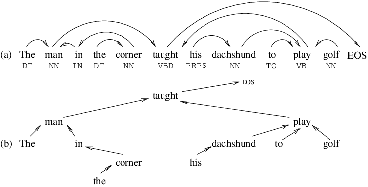
We begin with a brief review of the terminology. A bare-bones dependency structure is a sequence or string of $n$ words. Each word has been annotated with a tag, which indicates the word’s syntactic or semantic role, as well as a parent, which indicates where the word plays that role.

The parent of word $w$ is usually a pointer or link to another word in the string, which $w$ is said to modify. However, one word in the string (the “head” of the sentence) modifies nothing, and its parent is said to be the special symbol eos, an end-of-sentence mark that falls just past the end of the string (as word $n+1$). In addition, for the dependency structure to be well-formed, the parents must be assigned in such a way that the links never cross or form cycles. Each word is said to be the head of the contiguous substring formed by itself and all its descendants.

Figure 1 gives an example. Here the tags are simple part-of-speech tags as used in [Kucera & Francis 1967, Marcus et al. 1993]. It is possible to use a more articulated tag set, in order to achieve parses that are more precise and perhaps even more accurate. For example, in figure 1, dachshund’s tag might be extended so that it includes not only the part of speech, NN (noun), but also indications that this token of dachshund heads a definite NP and serves as a semantic agent. Aside from questions of smoothing sparse data, a large tag set can be used without changes to the model. However, the tag set used in the present experiments is merely a slightly refined version of the part-of-speech tags of [Kucera & Francis 1967, Marcus et al. 1993]. The refinements are described in §4.

The present paper compares various probability models. Each model describes a probability distribution over the space of all dependency structures for all word strings. When given a sentence of words $w_{1},w_{2},\ldots w_{n}$, the parser assigns respective tags $t_{1},t_{2},\ldots t_{n}$ and parents $p_{1},p_{2},\ldots p_{n}$ so as to maximize the probability $\Pr(\vec{w},\vec{t},\vec{p})$ of the resulting dependency structure (words, tags, and all). That is, the parser returns the highest-probability structure consistent with the given word string $\vec{w}$.

Under each model, the probability of a dependency structure $D$ can be described with reference to a notional process that generates $D$ through a unique sequence of structural choices. The probability of occurrence of $D$ is the probability of making the appropriate sequence of choices. Each choice is made randomly, with a probability conditioned only on certain aspects of the previously made choices.

Certain models do not achieve a 1-to-1 correspondence between choice sequences and legal dependency structures. In general, by assigning probability to a choice sequence, the model assigns a total probability to the class of all legal structures consistent with that sequence.

• •

  If classes of size $<1$ exist, the model is called leaky (or deficient): it allocates some probability to situations that can never legally arise.

• •

  If classes of size $>1$ exist, the model is called incomplete. It cannot be used to find the probabilities of individual structures, but only of classes. The parser therefore returns not the highest-probability structure, but an arbitrary representative of the highest-probability class. (For purposes of implementation, each parse is scored with the probability of its choice sequence, so that structures in the same class will suffer a tie that is broken arbitrarily.)

• •

  A third possibility is that the model may be inconsistent in that some classes overlap, i.e., a structure can be generated in more than one way. In this paper, however, only consistent models are considered; as stated above, each $D$ is generated through a unique sequence of structural choices.

Note that we may eliminate leakiness from a model by renormalizing its probabilities—that is, by defining $S$ as the total probability allocated to well-formed structures, and putting

Conveniently, since $S$ is a constant, maximizing $\Pr_{Normalized}(D)$ is the same as maximizing $\Pr(D)$ over just well-formed structures (or classes) $D$.

The general form of models A, B, and C is motivated in [Eisner 1996], to which the reader is referred for discussion. Figure 2 also gives an overview.

When defining precise versions of the models, we took care to make the comparison fair, by having the models condition their decisions on comparable information. In particular, all the models are sensitive to the following types of probabilistic interactions:

1. 1.

   Words are conditioned on their parents and on adjacent siblings in the dependency tree. Each child is attached (model A) or predicted (model B) or generated (model C) with a probability that varies with its ${\left\langle\mbox{word},\mbox{tag}\right\rangle}$ pair and the ${\left\langle\mbox{word},\mbox{tag}\right\rangle}$ pair of its parent. The probability also varies with the tag of the next-closest child of that parent, so that the model is sensitive to Markov-like dependencies among the successive children of a word.

2. 2.

   Words are conditioned on adjacent words in the string. Except in model C, which does not attend to string-local relations, each ${\left\langle\mbox{word},\mbox{tag}\right\rangle}$ pair is generated with probability conditional on the two ${\left\langle word,tag\right\rangle}$ pairs that immediately precede it in the string.

3. 3.

   When generating a sequence of ${\left\langle\mbox{word},\mbox{tag}\right\rangle}$ pairs, we begin in a distinguished start state, and end when we generate a distinguished “stop” symbol. (We generate such sequences in items 1–2 above: the sequence of children of a word is essentially regarded as the output of a Markov process, as is the sequence of words in the sentence.)

4. 4.

   Backoff and smoothing for sparse data (see §3) are performed similarly for all models. For example, in any model where the probability of a child depends on the identity of its neighboring sibling, we consider only a shortened version of that sibling’s tag.

The pseudocode given below is never actually run, but merely illustrates how, according to each model, a dependency structure $D$ with probability $\Pr(D)$ would be generated via a canonical series of probabilistic choices.

It is straightforward to reconstruct from the pseudocode how $\Pr(D)$ is defined for a given structure $D$. It is this value that the parser maximizes through dynamic programming, as described in [Eisner 1996].

Notation: $tw_{i}$ denotes the pair ${\left\langle w_{i},t_{i}\right\rangle}$, called a “tagged word.” The parents $p_{i}$ are represented as indices, so that $p_{i}=j$ means that the $i$th word modifies the $j$th word. The indices of the closest, 2nd-closest, 3rd-closest …right children of $w_{i}$ are sometimes denoted by $kid(i,1),kid(i,2),kid(i,3),\ldots$, and similarly the indices of the left children are $kid(i,-1),kid(i,-2),\ldots$. Also, we let $kid(i,0)$ denote $i$ itself, but by abuse of notation, $tw_{kid(i,0)}$ is taken to represent not $tw_{i}$ but a distinguished value ${\left\langle\mbox{\sc bokids},\mbox{\sc bokids}\right\rangle}$ that indicates the beginning of the left or right child sequence.

Model A: Bigram lexical affinities

Model A first generates a tagged sentence, using a simple trigram Markov model, as follows:

1.	$\Pr(D):=1$
2.	$tw_{-1}:=tw_{0}:={\left\langle\mbox{\sc bos},\mbox{\sc bos}\right\rangle}$   (* beginning-of-sentence *)
3.	n := 0
4.	for $n$ from 0
5.		choose $tw_{n+1}$ randomly from among all possible tagged words, conditioned on $tw_{n-1}$ and $tw_{n}$
6.		$\Pr(D):=\Pr(D)\times\Pr(tw_{n+1}\mid tw_{n-1},tw_{n})$
7.		if $tw_{n+1}={\left\langle\mbox{\sc eos},\mbox{\sc eos}\right\rangle}$ then break   (* end of sentence; don’t change $n$ *)

At this point, the model has generated a sequence of tagged words that has some probability $\Pr(\vec{w},\vec{t})$. In the second phase, the model will choose parents conditional on these tagged words, to get a full dependency structure with probability $\Pr(\vec{p}\mid\vec{w},\vec{t})\times\Pr(\vec{w},\vec{t})=\Pr(\vec{w},\vec{t},\vec{p})=\Pr(D)$.

For each pair of words (including the eos mark), the second phase of the model chooses whether to add a link between them. The order in which it makes these decisions is important, since links are not chosen independently. When $w_{i}$ decides whether to become a child of $w_{k}$, it can condition its decision on the next-closest child of $w_{k}$. This lets the model capture certain facts about subcategorization.

1.	for $k:=1$ to $n+1$
2.		(* choose the left children of $w_{k}$: each choice sees $w_{k}$ and the tag of the next-closest child *)
3.			c := 0   (* number of left children so far *)
4.			for $i:=k-1$ downto $1$
5.				choose whether $k$ should take $i$ as $kid(k,-(c+1))$, conditioned on $tw_{i}$, $tw_{k}$, and $tw_{kid(k,-c)}$
6.				$\Pr(D):=\Pr(D)\times\Pr(\mbox{the above yes/no choice}\mid tw_{i},tw_{k},tw_{kid(k,-c)})$
7.				if we chose “yes”
8.					then $c:=c+1$ and $kid(k,-c):=i$
9.		(* likewise choose the right children of $w_{k}$ *)
10.			c := 0   (* number of right children so far *)
11.			for $i:=k+1$ to $n$
12.				$\vdots$  (* as above *)

This model is leaky because many of the links are chosen independently of each other, so that it is possible to generate illegal dependency structures that feature words with no parents, words with multiple parents, link cycles, or crossing links.

Model B: Selectional preferences

The first phase of model B generates a tagged sentence, exactly as in model A. Thus each word and its tag are chosen based on local context.

The second phase corresponds to the pseudocode below. For each word it randomly and independently chooses a highly specific subcategorization/supercategorization frame from among all such frames, and then tries to link the words together so as to satisfy all the frames at once. The frame of a given word describes the parent and children that the word expects; it corresponds to a lexicalized version of a “disjunct” in link grammar [Sleator & Temperley 1991] or a “supertag” in probabilistic tree-adjoining grammar [Srinivas & Joshi 1994].

A tagged word $tw$ chooses the subcategorization part of its frame by generating a Markov sequence of desired left children and another Markov sequence of desired right children, that is, of tagged words that $tw$ expects to match the heads of its complements and adjuncts. It gets the supercategorization part of its frame by choosing a tagged word that it expects to match its parent. All generation probabilities are further conditioned on $tw$ itself.

1.	for $k:=1$ to $n+1$
2.		(* choose a sequence of tagged words that $tw_{k}$ will require its left children to match *)
		(* each choice sees $tw_{k}$ and the tag of the next closest child *)
3.			for $c$ from $0$
4.				choose a tagged word $\hat{tw}(k,-(c+1))$ that $kid(k,-(c+1))$ will have to match;
					choice is made over all tagged words in the vocabulary, conditioned on $tw_{k}$ and $\hat{tw}(k,-c)$
5.				$\Pr(D):=\Pr(D)\times\Pr(\hat{tw}(k,-(c+1))\mid tw_{k},\hat{tw}(k,-c))$
6.				if $\hat{tw}(k,-(c+1))={\left\langle\mbox{\sc eokids},\mbox{\sc eokids}\right\rangle}$ then break   (* end of left child sequence *)
7.		(* similarly choose a sequence of tagged words that $w_{k}$ will require its right children to match *)
8.			$\vdots$  (* as above *)
9.		if $k\leq n$
10.			choose a tagged word $\hat{tw}$ that $w_{k}$ will require its parent to match, conditioned on $w_{k}$
11.			$\Pr(D):=\Pr(D)\times\Pr(\hat{tw}\mid w_{k})$
12.	If possible, choose parents $p_{1},p_{2},\ldots p_{n}$ in any way so that the parent and children of each word
		$w_{k}$ satisfy the frame for $w_{k}$ generated above.

This model is leaky: step Model B: Selectional preferences may fail, because the right words to satisfy the frames are not present, or else cannot be linked together without crossing links. In that case, some probability mass has been assigned to an impossible structure. Note in particular that each tagged word is generated two or more times—once during the generation of a tagged sentence and once for each of the other words it links to as parent or child. The structure can be legal only if the same tagged word is generated on all these occasions. Furthermore, the model is incomplete, because there may be more than one way to carry out step Model B: Selectional preferences.³³ 3 For example, if we were parsing arithmetic expressions, the 9-word string $a-x-p-q-y$ (not a minimal example) would admit both of the following dependency strucures, which correspond to $a-(x-((p-q)-y))$ and $(a-((x-(p-q))-y))$, and which reflect exactly the same frame for each word token $w_{i}$: - a - x - - p q y          - a - - x - p q y It can be proved that if each word’s frame specifies not only the number of its left and right children, but also the direction (left or right) of its parent, then at most one dependency structure is possible in step Model B: Selectional preferences and the model is no longer incomplete. Unfortunately, §5 shows that augmenting frames with parental direction hurts the model’s performance substantially.

Model C: Recursive generation

Model C is based on the idea that each word generates its actual children, in just the same way that in Model B each word generates its desired children (subcategorization frame). Given a tagged word $tw$, we can generate its left children $tw(-1),tw(-2),\ldots$ as a Markov sequence of tagged words further conditioned on $tw$, and its right children likewise.⁴⁴ 4 We use this notation for convenience, rather than describing how to work out the actual indices of the children, which is straightforward. The process is repeated recursively on those words, yielding a tree as in Figure 1b. The process consists of calling generate on the pair ${\left\langle\mbox{\sc eos},\mbox{\sc eos}\right\rangle}$, where generate$(tw)$ is defined below.

1.	(* choose $tw$’s sequence of left children, $tw(-1),tw(-2),\ldots$; each choice sees $tw$ and the tag of the next closest child *)
2.		for $c$ from $0$
3.			choose $tw(-(c+1))$ conditional on $tw$ and $tw(-c)$
4.			$\Pr(D):=\Pr(D)\times\Pr(tw(-(c+1))\mid tw,tw(-c))$
5.			if $tw(-(c+1))={\left\langle\mbox{\sc eokids},\mbox{\sc eokids}\right\rangle}$ then break   (* end-of-left-child-sequence *)
6.			generate$(tw(-(c+1)))$
7.	(* similarly choose a sequence of tagged words that $w_{k}$ will require its right children to match *)
8.		$\vdots$  (* as above *)

This top-down, generative model is neither leaky nor incomplete.⁵⁵ 5 An interesting variation would be to do the generation in depth-first order, so that the $c$th child of a word (on either side of the word) would be chosen based on the word, its left sibling, and the two tagged words that immediately string-precede the child’s subtree. This would allow the model to take string-local context into account in the same way as models A and B. This variation has not been tested experimentally. While it can be implemented within the parsing framework of [Eisner 1996], it leads to somewhat larger span signatures, meaning that its time and space requirements suffer from a fairly large (though not wholly unreasonable) constant factor. On the other hand, the model could consider untagged versions of the preceding words at no extra cost (Mike Collins, p.c.).

Model D: Realistic selectional preferences

It is simplest to regard this model as a variant of model B. When a word in model B generates its subcategorization frame (line Model B: Selectional preferences), it does so in ignorance of the words that are actually available to fill such a frame—although those words have already been generated. A better model would generate a string of words as model B does, and then have each word select a sequence of real children (tokens) from among the remaining words (cf. model A) rather than generating a sequence of desired children (types). Ideally, the latter phase of this model would look as follows:

1.	for $k:=1$ to $n+1$
2.		(* select the left-child sequence of word $k$ from among existing words *)
3.			for $c$ from $0$
4.				choose $kid(k,-(c+1))$ from the set $C=\{1,2,\ldots kid(k,-c)-1,{\sc eokids}\}$
					i.e., the choices are the words to the left of $kid(k,-c)$ plus the distinguished symbol eokids
5.				$\Pr(D):=\Pr(D)\times\Pr(kid(k,-(c+1))\mid C,tw_{k},tw_{kid(k,-c)})$
6.				if $kid(k,-(c+1))={\sc eokids}$ then break   (* end of left child sequence *)
7.		(* similarly select the right-child sequence of word $k$ *)
8.			$\vdots$  (* as above *)
9.		(* no parent or supercategorization frame is chosen *)

This model does generate structures with crossing links, so it is leaky, but less so than model B.

The difficulty with the description above lies in estimating $\Pr(kid(k,-(c+1))\mid C,tw_{k},tw_{kid(k,-c)})$ in line Model D: Realistic selectional preferences. This is the probability of choosing a particular next child $i$ (perhaps the special choice eokids) given the particular set $C$ of available remaining children.

The model of [Collins 1996] faces a similar problem, which Collins addresses essentially by using the backed-off probability $\Pr(kid(k,-(c+1))=i\mid tw_{i},tw_{k})$. That is, when tokens labeled like $tw_{i}$ and $tw_{k}$ are in the sentence, what is the probability that the former links to the latter?

Model D also backs off, but in a more nuanced way, to $\Pr(kid(k,-(c+1))=i\mid tw_{i},(i\in C),tw_{k},tw_{kid(k,-c)})$. That is, when tokens labeled like $tw_{i}$ and $tw_{k}$ are in the sentence, what is the probability that the former links to the latter as the $(c+1)$st left child—given that the former does fall to the left of the latter’s $c$th left child, which is labeled like $tw_{kid(k,-c)}$? These last two conditions are disregarded by [Collins 1996].

Note that the more nuanced backoff of Model D enables the model to capture probabilistic interactions among successive children of $w_{k}$, just as models A–C do. The most important such interaction is that between the outermost child of $w_{k}$ and eokids. This interaction serves to capture such facts as arity—the fact that $w_{k}$, depending on whether it has an existing child of a particular type, may require or forbid an additional child.

For purposes of computation, one might regard model D as a variant of model A. The difference (other than the use of eokids) is that in line Model A: Bigram lexical affinities of model A, we will continue to multiply $\Pr(D)$ by the probabilities that the links we have accepted are indeed right, but not by the probabilities that the links we have rejected are indeed wrong. Thus, the probability that model D assigns to a structure is the probability that model A would select at least the $n$ links found in the structure, and perhaps others as well. It is difficult to give an independent justification of the model along these lines: note especially the problem that if model A assigns some probability to a structure with $m>n$ links, then this probability is added separately to each of the $\left(\begin{array}[]{@{}c@{}}{m}\\ {n}\end{array}\right)$ structures with some $n$ of these links.

The general approach is to decompose a probability of the form

into a product of the form

Each of the factors in this product is then estimated separately as a conditional probability.

To estimate a conditional probability, we may have to back off, i.e., reduce the condition so that it is less detailed. For example, to estimate the third factor above, we might choose to reduce its condition $B,C,D,E$ to simply $B$, or perhaps to $D,E$, depending on the independence assumptions that we believe are justified. That is, we might estimate $\Pr(A\mid B,C,D,E)$ as $\Pr(A\mid B)$ or $\Pr(A\mid D,E)$ respectively.

Severe reductions throw away much potentially relevant information about the conditions that obtain in the sentence, so they are justified only by sparse data. To allow a dynamic tradeoff between sensitive conditions and sufficient data, each conditional probability is estimated using an associated list of reductions, which are increasingly more severe. The first reduction on the list keeps all or most of the original condition; later reductions throw away more and more of this information.

How is this list of reductions used? Suppose that we wish to estimate $\Pr(A\mid B,C,D,E)$, and that the first (least severe) reduction reduces the condition to $D,E$. If this is the only reduction, we return the estimate $\frac{count(A\&D\&E)+0.005}{count(D\&E)+0.5}$, an approximation to $\Pr(A\mid D,E)$ that is based on training data counts. However, if there are additional reductions, we recursively compute an estimate $p$ using the remaining list of reductions, and return the estimate $\frac{count(A\&D\&E)+3p}{count(D\&E)+3}$. Thus, the coarse, backed-off estimate $p$ has the weight of 3 additional observations of the specific context $D,E$. If the specific context $D,E$ has been frequently observed, it will largely override the coarse estimate $p$ [Collins 1996].⁶⁶ 6 For efficiency, we do not bother to add $3p$ to the numerator and 3 to the denominator, or even to compute $p$, in the event that $count(D\&E)$ is large $\geq 8$. This policy may actually be unwise, given that the numerator may be zero even when the denominator is large.

In describing the factors and reductions, we assume the following functions:

$tag(tw)$:

Given a tagged word, extract the tag.⁷⁷ 7 While it is not done here, the $tag$ function can be modified so that if $tw$ is a “special” word, such as a high-frequency or closed-class word, then $tag(tw)=tw$. This is equivalent to giving special words their own tags.

$word(tw)$:

Given a tagged word, extract a lowercase version of the word.

$cap(tw)$:

Given a tagged word, extract information about its capitalization. $cap(tw)$ can take on four values:

DOWN

all-lowercase

UP

all-caps (and at least two letters)

INIT

$tw$ is the first non-punctuation word in a sentence, and just its first letter is capitalized.

CAP

all other cases, in particular unambiguously capitalized or mixed-case words

$short(tag)$:

A function that maps specific tags to more general tags: for example, $short(\verb+JJR+)=short(\verb+JJS+)=\verb+ADJ+$. The corpus we use has 71 tags but only 22 shortened tags.

$tiny(tag)$:

A more aggressive version of $short(tag)$, which groups the 71 tags into just 7 equivalence classes: Noun, Verb, Noun Modifier, Adverb, Preposition, Wh-Word, and Punctuation.

$dist(i,j)$:

The distance between word positions $i$ and $j$, represented as one of the four ranges 1, 2, 3–6, and 7–$\infty$.

We now turn to the probabilities that must be generated.

1. 1.

   Models A, B, and D must each generate a string of tagged words according to a trigram model. The crucial probability is computed via the following factors and reductions:

   	$\displaystyle\Pr(tw_{k+1}\mid tw_{k},tw_{k-1})$	$\displaystyle=$	$\displaystyle\Pr(cap(tw_{k+1}),word(tw_{k+1}),tag(tw_{k+1})\mid tw_{k},tw_{k-1})$
   		$\displaystyle=$	$\displaystyle\Pr(tag(tw_{k+1})\mid tw_{k},tw_{k-1})$
   			$\displaystyle\hskip 32.52127pt\mbox{reduction list}:\begin{array}[]{|l|}\hline\cr tag(tw_{k}),tag(tw_{k-1})\\ \hline\cr tag(tw_{k})\\ \hline\cr short(tag(tw_{k}))\\ \hline\cr\end{array}$
   			$\displaystyle\times\Pr(word(tw_{k+1})\mid tag(tw_{k+1}),tw_{k},tw_{k-1})$
   			$\displaystyle\hskip 32.52127pt\mbox{reduction list}:\begin{array}[]{|l|}\hline\cr tag(tw_{k+1})\\ \hline\cr\end{array}$
   			$\displaystyle\times\Pr(cap(tw_{k+1})\mid word(tw_{k+1}),tag(tw_{k+1}),tw_{k},tw_{k-1})$
   			$\displaystyle\hskip 32.52127pt\mbox{reduction list}:\begin{array}[]{|l|}\hline\cr word(tw_{k+1}),tag(tw_{k+1})\\ \hline\cr tag(tw_{k+1})\\ \hline\cr\end{array}$

   Notice that if we consider only the first reduction for each factor, the above specifies the estimate $\Pr(t_{k+1}\mid t_{k},t_{k-1})\times\Pr(w_{k+1}\mid t_{k+1})$, which is a standard trigram model [Church 1988, and others].

2. 2.

   Model B must also estimate $\Pr(tw_{parent}\mid tw_{child})$. This is formally the same problem as estimating $\Pr(tw_{k+1}\mid tw_{k})$, and is handled as a special case of the $\Pr(tw_{k+1}\mid tw_{k},tw_{k-1})$ computation above.

3. 3.

   Models B and C must generate $tw_{k}$’s sequence of children in direction $dir$, where $dir$ is either Left or Right. For concreteness let us assume that $dir$=Right, so that the children are $kid(k,1),kid(k,2),\ldots$.

   	$\displaystyle\Pr(tw_{kid(k,c+1)}\mid tw_{k},tw_{kid(k,c)},dir)$
   		$\displaystyle=$	$\displaystyle\Pr(cap(tw_{kid(k,c+1)}),word(tw_{kid(k,c+1)}),tag(tw_{kid(k,c+1)})\mid tw_{k},tw_{kid(k,c)},dir)$
   		$\displaystyle=$	$\displaystyle\Pr(tag(tw_{kid(k,c+1)})\mid tw_{k},tw_{kid(k,c)},dir)$
   			$\displaystyle\hskip 32.52127pt\mbox{reduction list}:\begin{array}[]{|l|}\hline\cr tw_{k},short(tag(tw_{kid(k,c)}))),dir\\ \hline\cr\left\{\begin{array}[]{l}tw_{k},dir\\ tag(tw_{k}),short(tag(tw_{kid(k,c)})),dir\\ \end{array}\right.\\ \hline\cr short(tw_{k}),dir\\ \hline\cr\end{array}\ \ \ \mbox{(see below)}$
   			$\displaystyle\times\Pr(word(tw_{kid(k,c+1)})\mid tag(tw_{kid(k,c+1)}),tw_{k},tw_{kid(k,c)},dir)$
   			$\displaystyle\hskip 32.52127pt\mbox{reduction list}:\begin{array}[]{|l|}\hline\cr tag(tw_{kid(k,c+1)}),tw_{k},dir\\ \hline\cr tag(tw_{kid(k,c+1)}),tag(tw_{k}),dir\\ \hline\cr tag(tw_{kid(k,c+1)})\\ \hline\cr\end{array}$
   			$\displaystyle\times\Pr(cap(tw_{kid(k,c+1)})\mid word(tw_{kid(k,c+1)}),tag(tw_{kid(k,c+1)}),tw_{k},tw_{kid(k,c)},dir)$
   			$\displaystyle\hskip 32.52127pt\mbox{reduction list}:\begin{array}[]{|l|}\hline\cr word(tw_{kid(k,c+1)}),tag(tw_{kid(k,c+1)})\\ \hline\cr tag(tw_{kid(k,c+1)})\\ \hline\cr\end{array}$

   In a version of model B or C in which we generate not only the children of a head but also their desired distance from the head, the objective is to find $\Pr(dist(k,kid(k,c+1)),tw_{kid(k,c+1)}\mid tw_{k},tw_{kid(k,c)},dir)$. For this version we must multiply by an additional factor:

   	$\displaystyle\times\Pr(dist(k,kid(k,c+1))\mid tw_{kid(k,c+1)},tw_{k},tw_{kid(k,c)},dir)$
   	$\displaystyle\hskip 32.52127pt\mbox{reduction list}:\begin{array}[]{|l|}\hline\cr tw_{kid(k,c+1)},tag(tw_{k})\\ \hline\cr tag(tw_{kid(k,c+1)}),tag(tw_{k})\\ \hline\cr\end{array}$

   Note that while model C is ordinarily not a leaky model, adding this factor will make it leaky.

   Note that one of the reductions above has a disjunctive condition, whose disjuncts are grouped by a bracket {. Disjunction is useful because it is not always possible to know which part of the original condition should be thrown away in a reduction in order to overcome sparse data. Using this disjunctive reduction, we estimate the desired factor $\Pr(tag(tw_{kid(k,c+1)})\mid tw_{k},tw_{kid(k,c)},dir)$ as follows:

   $$\frac{count(tag(tw_{kid(k,c+1)}),tw_{k},dir)+count(tag(tw_{kid(k,c+1)}),tag(tw_{k}),short(tag(tw_{kid(k,c)})),dir))}{count(tw_{k},dir)+count(tag(tw_{k}),short(tag(tw_{kid(k,c)})),dir)}$$

   That is, we compute a numerator and denominator for each disjunct separately, as if that disjunct were the entire reduction, and find our estimate by adding the numerators and adding the denominators. The disjunct with the greater denominator (i.e., whose condition is more common) will have the greater influence on our estimate [Collins & Brooks 1995].

4. 4.

   Models A and D must be able to decide, for words at positions $k$ and $i>k$ such that $k$ already has $c$ children between $k$ and $i$, whether $i$ is the $(c+1)$st child of $k$:

   	$\displaystyle\Pr(\mbox{link from $i$ to $k$}\mid tw_{i},tw_{k},tw_{kid(k,c)})$
   			$\displaystyle\hskip 32.52127pt\mbox{reduction list}:\begin{array}[]{|l|}\hline\cr word(tw_{i}),tag(tw_{i}),word(tw_{k}),tag(tw_{k}),short(tag(tw_{kid(k,c)}))\\ \hline\cr\left\{\begin{array}[]{l}tag(tw_{i}),word(tw_{k}),tag(tw_{k}),short(tag(tw_{kid(k,c)}))\\ word(tw_{i}),tag(tw_{i}),tag(tw_{k}),short(tag(tw_{kid(k,c)}))\\ word(tw_{i}),tag(tw_{i}),word(tw_{k}),tag(tw_{k})\\ \end{array}\right.\\ \hline\cr tag(tw_{i}),tag(tw_{k}),short(tag(tw_{kid(k,c)}))\\ \hline\cr tag(tw_{i}),tag(tw_{k}),tiny(tag(tw_{kid(k,c)}))\\ \hline\cr\end{array}$

   It is also possible to construct a version of these models that conditions on distance, in which case we use the following:

   	$\displaystyle\Pr(\mbox{link from $i$ to $k$}\mid dist(i,k),tw_{i},tw_{k},tw_{kid(k,c)})$
   			$\displaystyle\hskip 32.52127pt\mbox{reduction list}:\begin{array}[]{|l|}\hline\cr dist(i,k),word(tw_{i}),tag(tw_{i}),word(tw_{k}),tag(tw_{k}),short(tag(tw_{kid(k,c)}))\\ \hline\cr\left\{\begin{array}[]{l}dist(i,k),tag(tw_{i}),word(tw_{k}),tag(tw_{k}),short(tag(tw_{kid(k,c)}))\\ dist(i,k),word(tw_{i}),tag(tw_{i}),tag(tw_{k}),short(tag(tw_{kid(k,c)}))\\ dist(i,k),word(tw_{i}),tag(tw_{i}),word(tw_{k}),tag(tw_{k})\\ \end{array}\right.\\ \hline\cr\left\{\begin{array}[]{l}tag(tw_{i}),word(tw_{k}),tag(tw_{k})\\ word(tw_{i}),tag(tw_{i}),tag(tw_{k})\\ \end{array}\right.\\ \hline\cr dist(i,k),tag(tw_{i}),tag(tw_{k}),short(tag(tw_{kid(k,c)}))\\ \hline\cr dist(i,k),tag(tw_{i}),tag(tw_{k}),tiny(tag(tw_{kid(k,c)}))\\ \hline\cr\end{array}$

References

- [Black et al.1991] E. Black et al. 1991. A procedure for quantitatively comparing the syntactic coverage of English grammars. Proceedings of the February 1991 DARPA Speech and Natural Language Workshop.
- [Caraballo & Charniak 1996] Sharon Caraballo and Eugene Charniak. 1996. New figures of merit for best-first probabilistic chart parsing. Ms., Brown University (submitted to Computational Linguistics).
- [Chen & Goodman 1996] Stanley Chen and Joshua Goodman. 1996. An empirical study of smoothing techniques for language modeling. In Proceedings of the 34th Annual Meeting of the Association for Computational Linguistics, Santa Cruz, July. cmp-lg/9606011.
- [Church 1988] Kenneth W. Church. 1988. A stochastic parts program and noun phrase parser for unrestricted text. In Proceedings of the 2nd Conf. on Applied Natural Language Processing, 136–148, Austin, TX. Association for Computational Linguistics, Morristown, NJ.
- [Collins 1996] Michael J. Collins. 1996. A new statistical parser based on bigram lexical dependencies. Proceedings of the 34th ACL, Santa Cruz, July, 184–191. cmp-lg/9605012.
- [Collins & Brooks 1995] M. Collins and J. Brooks. 1995. Prepositional phrase attachment through a backed-off model. Proceedings of the Third Workshop on Very Large Corpora, 27–38. cmp-lg/9506021.
- [Eisner 1996] Jason M. Eisner. 1996. Three new probabilistic models for dependency parsing: an exploration. Proceedings of the 16th International Conference on Computational Linguistics (COLING-96), Copenhagen, August, 340–345. cmp-lg/9706003.
- [Kucera & Francis 1967] H. Kucera and W.N. Francis. 1967. Computational Analysis of Present-Day American English. Providence, RI: Brown University Press.
- [Lin 1995] Dekang Lin. 1995. A dependency-based method for evaluating broad-coverage parsers. In Proceedings of the International Joint Conference on Artificial Intelligence.
- [Marcus et al. 1993] M. Marcus, B. Santorini, and M. Marcinkiewiecz. 1993. Building a large annotated corpus of English: the Penn Treebank. Computational Linguistics, 19(2):313–330.
- [Marcus et al. 1994] M. Marcus, G. Kim, M. A. Marcinkiewicz, R. MacIntyre, A. Bies, M. Ferguson, K. Katz, B. Schasberger. 1994. The Penn Treebank: Annotating predicate-argument structure. Proceedings of the 1994 Human Language Technology Workshop, 110–115.
- [Mooney 1996] Rayoond J. Mooney. 1996. Comparative experiments on disambiguating word senses: An illustration of the role of bias in machine learning. Proceedings of the Conference on Empirical Methods in Natural Language Processing, University of Pennsylvania, May. cmp-lg/9612001.
- [Ratnaparkhi 1996] Adwait Ratnaparkhi. 1996. A maximum-entropy model for part-of-speech tagging. Conference on Empirical Methods in Natural Language Processing.
- [Sleator & Temperley 1991] Daniel Sleator and Davy Temperley. 1991. Parsing English with a Link Grammar. Technical report CMU-CS-91-196. CS Dept., Carnegie Mellon Univ. cmp-lg/9508004.
- [Srinivas & Joshi 1994] B. Srinivas and Aravind Joshi. 1994. Disambiguation of Super Parts of Speech (or Supertags): Almost Parsing. Proceedings of COLING 94, Kyoto, Japan, August. cmp-lg/9410029.