The Observed Size and Shape of GRB Afterglow
Abstract
The detection of delayed emission in X-ray, optical and radio wave length, “afterglow”, following a -ray burst can be described by the emission of a relativistic shell decelerating upon collision with the ISM. We show that the observed radiation surface have well defined bright edges. We derive an explicit expression for the size as a function of time, and obtain the surface brightness distribution. This might be directly observed if the burst occurs at small redshift so that its radio signal can be resolved. The size and shape are relevant for detailed analysis of scintillation or microlensing. We show that the effective Lorentz factor depends on the observed frequency and it is higher for frequencies above the synchrotron typical frequency (optical and X-ray) than for low frequencies (radio). Consequently transition to non relativistic evolution, will be observed first in low frequencies and only a factor of later in the high frequencies.
Keywords:
-rays: burst; hydrodynamics: shocks; relativity1 Introduction
The detection of delayed emission in X-ray optical and radio wave length, “afterglow”, following a -ray burst is reasonably described by the emission of a relativistic shell decelerating upon a collision with the ISM (Waxman 1997a,b, Wijers Rees and Mészáros 1997, Katz and Piran 1997). The radio observations show substantial oscillations of order unity over the first few weeks (Frail et. al. 1997), while the optical measurements at the same time follow a smooth regular decline. It is therefor likely that the nature of these oscillations is not intrinsic to the source. These oscillations might be explained by scintillation in our galaxy. Goodman’s estimates (1997) show that the size of the observed emitter is in the limit between being a large object, subject only to refractive scintillation, and being a small one, subject to diffractive scintillation that can account for fluctuations of order unity. In order to correctly account for this scintillation a good estimate for the size of the observed object is needed. In addition, the size of the object is relevant for estimates of the observed luminosity if the emission is self absorbed (Katz & Piran 1997). The size is also important in concern with microlensing (Loeb & Perna 1997). In section 2 we show that the observed radiation has well defined boundaries and derive an explicit expression for its size. In section 3 we discuss the brightness distribution within this limited size. We find the flux averaged radius and Lorentz factor of the material emitting the radiation. We show that this effective emission radius for observed frequencies above the peak frequency is smaller than for observed frequencies below the peak frequency.
2 The Size of The Afterglow
We consider first the well know result (Rees 1966) of the observed size of a thin shell with constant velocity . This relation is simple to derive and it gives the basic picture. It is also appropriate for non relativistic velocities. After a time the shell is located at radius . A photon that is emitted at an angle from the line of sight (connecting the observer and the source) will reach the observer at time
| (1) |
where . This expression describes the locus of points from which the radiation reaches the observer at the same time (see upper frame of Figure 1). It is an ellipse whose long axis is along the line of sight. The source is located at the far focal point. The observed size of the emitting area is the small axis of the ellipse .
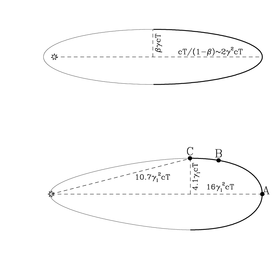
In the afterglow scenario a shell accumulates ISM mass and decelerates with . Due to the accumulation of mass, the Lorentz factor of the shock front is higher than the Lorentz factor of the material behind it by a factor of . As we have recently pointed out (Sari 1997), the relation between the observed time of arrival of photon from the line of sight and the radius at which it was emitted is , where is the Lorentz factor of the material immediately behind the shock. The subscript indicates that this relation is valid only for photons arriving from the line of sight. An equivalent expression relating and the time of emittance is
| (2) |
The arrival time of a photon emitted at an angle is given by
| (3) |
Solving equation 2 and 3 we have
| (4) |
Substituting =, the above equation yields
| (5) |
Equation 5 is the decelerating analogy of the ellipse given in equation 1 for a constant velocity shell. It describes an elongated “egg-shape” shown in the lower frame of Figure 1.
The relevant size in the context of scintillation or microlensing would be the distance from the line of sight :
| (6) |
The maximal value of the expression is obtained at
| (7) |
where
| (8) |
This should be compared with the constant velocity shell . A substitution of the expression for (Sari 1997) obtained by using the self similar solution of Blandford & McKee (1976) yields:
| (9) |
This result is quite robust as it depend very weakly on the energy in the system erg and the ISM particle density . The only assumptions used are adiabatic evolution described by the Blandford and McKee self similar solution, and the assumption of high Lorentz factor.
3 The Surface Brightness Distribution
Equation 9 gives the maximal from which radiation will reach the observer at a given observer time. The distribution of the surface brightness within this radius requires additional assumptions concerning the emitted spectrum.
Consider a system with an isotropic luminosity , at some frequency (both in the fluid comoving frame), that is moving with Lorentz factor in a direction with width relative to the line of sight. Each photon of frequency will be Lorentz boosted to frequency . Using Lorentz transformation, the observed flux at distance from the source satisfies:
| (10) |
A spherical system, with a luminosity in its local frame, is simply a collection of such directed systems. The luminosity coming from an angle with around is so that
| (11) |
Since we are interested in the radiation coming from any per unit area (surface brightness) this expression must be multiplied by
| (12) |
where we can use equations 5 and 6 to evaluate the derivatives. Using equation 5 and assuming , we can approximate
| (13) |
So that
| (14) |
We now assume that the luminosity in the local frame is changing with radius and frequency as
| (15) |
With this assumption the surface brightness coming from a radius is proportional to
| (16) |
This is also a function of using equation 6. Note that the function is double valued. For each there are two values of , one from the front of the expanding shell and one from its back. On the transition point, where , we get the relativistic version of limb brightening, as the denominator of the second term in equation 16 vanishes. The limbs in the relativistic version are not the edges of the surface in a given time as in the nonrelativistic case but the edges of surface from which photons arrive in a given observed time.
The assumption of equation 15 is justified for frequencies which are far from the typical synchrotron frequency (either above or below). Fortunately these are two relevant cases as the radio range is below the typical frequency for few months while the optical bands are above the typical frequency after about 1 day. Assuming that the electrons are not cooling significantly we find that the luminosity is proportional to the number of electrons times the power produced by each electron . This is emitted at a typical frequency of . The luminosity at the typical frequency is therefor
| (17) |
The synchrotron low energy tail (assuming that the electrons are neither cooling nor self absorbed) is so that for
| (18) |
At the high energy tail, assuming that the electron distribution is a power law with equal energy per decade we get
| (19) |
Figure 2 depicts the observed surface brightness for these two cases of low and high frequencies. In both cases the surface brightness diverges at . In the low frequency case the surfaces brightness in the center is about half the average surface brightness while in the high frequencies it is only about 10%. Practically all the luminosity at high frequencies is emitted from a ring while at low frequencies it is spread more uniformly. This qualitative difference might be intuitively understood as for high frequencies the luminosity is decaying in time so that emission from a lower radius (coming off the line of sight) is enhanced relative to the emission from the line of sight.

As seen from figure 1, the radiation at a given observed time comes from a large range of radii . However, using equation 16 one can calculate the flux averaged radius of emission or the flux averaged perpendicular emission radius . The Lorentz factor at the average radius can then be calculated by . For low frequencies we find
| (20) |
while for high frequencies
| (21) |
Therefor radiation arriving the observer at a certain time in a frequency band above the peak frequency, was emitted on average from lower radius, higher Lorentz factor and outer , than radiation arriving to the observer at the same time in an energy band below the peak. One can now find the relation between the typical radius , the typical Lorentz factor and the observed time . For low frequencies:
| (22) |
while for high frequencies
| (23) |
These replace the usual relation . The coefficient in the denominator depends on the frequency observed. Its range is between (for frequencies far below the peak frequency) and (for frequencies far above the peak frequency). Therefor for the peak frequency itself we expect the coefficient to be some average of these two extreme values.
4 Conclusions
We have explored the spatial shape of the radiation emitted from a decelerating relativistic shell in its adiabatic evolution . Using the self similar solution which gives the exact proportionality constant we have arrived at an explicit expression for the observed size of the emission as a function of time.
We have further analyzed the observed surface brightness in two extreme cases of frequencies far below and far above the typical synchrotron frequency. These two extremes are of practical importance as the radio is below the typical synchrotron frequency for few month and the optical is above the typical synchrotron frequency after about a day. We showed that this emission has sharp well defined edges. The edges are brighter than the center as a result of a relativistic version of the limb brightening effect.
The surface brightness for frequencies below the synchrotron typical frequency was shown to be more uniform than in the high frequency range in which most of the radiation comes from a small region near the limbs. The exact shape is relevant for a detailed scintillation theory. Furthermore, in the case of a “nearby” burst with it is likely that the radio source will be resolved, and a direct observation of the surface brightness will be possible.
The relation between the emission radius, the Lorentz factor and the observed time is not well defined as there is a large range of radii from which the emission reaches the observer at the same time. However taking the flux averaged radius of emission and the Lorentz factor at the average radius we find where for the high frequency limit and in the low frequency limit. These values of are smaller than the coefficient obtained from the line of sight (Sari 1997) however larger than the usual value of .
The effective Lorenz factor for high frequencies is larger by than the effective Lorentz factor for low frequencies. The transition to the non relativistic stage and the effect of finite size jet (Rhoads 1997) both depend on the Lorentz factor. Since the observed time , these effects would be observable in the radio at about a factor of two earlier than they would be observed in the optical range.
- (1) Blandford, R. D. & McKee, C. F. 1976, Phys. of Fluids, 19, 1130
- (2) Frail, D. A., Kulkarni, S. R., Nicastro, L., Feroci, M., Taylor, G. B. 1997, Nature, in press.
- (3) Goodman, J. 1997, submitted to New Astronomy, astro-ph/9706084
- (4) Katz & Piran 1997, ApJdecember first issue, astro-ph/9706141.
- (5) Loeb, A. & Perna, R. 1997, submitted to ApJLetters, asto-ph9708159
- (6) Mészáros, P. & Rees, M. 1997, ApJ, 476, 232
- (7) Rees, M. 1966, Nature, 211, 468.
- (8) Rhoads J. E., astro-ph/9705163.
- (9) Sari, R. 1997, ApJL, in press.
- (10) Wijers, R. A. M. P., Rees M. & Mészáros, P. 1997, astro-ph/9704153
- (11) Waxman, E. 1997a, ApJ, 485, L5.
- (12) Waxman, E. 1997b, Nature, submitted, astro-ph/9705229