Nonlinear electrodynamics and the gravitational redshift of highly magnetised neutron stars
Abstract
We show that nonlinear electrodynamics (NLED) modifies in a fundamental basis the concept of gravitational red-shift (GRS) as it was introduced by Einstein’s general relativity. The effect becomes apparent when light propagation from super strongly magnetized compact objects, as pulsars, is under focus. The analysis, here based on the (exact) nonlinear Lagrangean of Born & Infeld (1934), proves that alike from general relativity (GR); where the GRS independs on any background magnetic () field, when NLED is taken into the photon dynamics an effective GRS appears, which happens to decidedly depend on the -field pervading the pulsar. The resulting GRS tends to infinity as the -field grows larger, as opposed to the Einstein prediction. As in astrophysics the GRS is admittedly used to infer the mass-radius relation, and thus the equation of state of a compact star, e.g. a neutron star (Cottam, Paerels & Mendez 2002), this unexpected GRS critical change may misguide observers to that fundamental property. Hence, a correct procedure to estimate those valuous physical properties demands a neat separation of the NLED effects from the pure gravitational ones in the light emitted by ultra magnetised pulsars.
Keywords:
Gravitation: redshift — nonlinear methods: electrodynamics — stars: neutron — pulsars: generalAugust 11, 2026
1 INTRODUCTION
The idea that the nonlinear electromagnetic interaction, i. e., light propagation in vacuum, can be geometrized was developed by Novello et al. (2000) and Novello & Salim (2001). Since then a number of physical consequences for the dynamics of a variety of systems have been explored. In a recent paper, Mosquera Cuesta & Salim (2003,2004) presented the first astrophysical context where such nonlinear electrodynamics effects were accounted for: the case of a highly magnetized neutron star or pulsar. In that paper NLED was invoked a là Euler-Heisenberg, which is an infinite series expansion of which only the first nonlinear term was used for the analisys. An immediate consequence of that study was an overall modification of the space-time geometry around the pulsar as “perceived” by light propagating out of it. This translates into a fundamental change of the star surface redshift, the GRS, which might have been inferred from the absorption (or emission) lines observed in a super magnetized pulsar by Ibrahim et al. (2002;2003). The result proved to be even more dramatic for the so-called magnetars: pulsars said to be endowed with magnetic () fields higher then the Schafroth quantum electrodynamics critical -field. In this Letter we demonstrate that the same effect still appears if one calls for the NLED in the form of the one rigorously derived by Born & Infeld (1934), which is based on the special relativistic limit to the velocity of approaching of an elementary charged particle to a pointlike electron. As compared to our previous results, here we stress that from the mathematical point of view the Born & Infeld (1934) NLED is described by an exact Lagrangean whose dynamics has been successfully studied in a wide set of physical systems (Delphenich 2003). The analysis presented next proves that this physics affects not only the magnetar electrodynamics (our focus here) but also that one of newly born; highly magnetised proto-neutron stars and the dynamics of their progenitor supernovae.
2 Neutron star mass-radius relation
Neutron stars (NSs), formed during the death throes of massive stars, are among the most exotic objects in the universe. They are supposed to be composed of essentially neutrons, although some protons and electrons are also required in order to guarantee stability against Pauli’s exclusion principle for fermions. As remnants of supernova explosions or accretion-induced-collapse of white dwarfs, they are (canonical) objects with extremely high density g cm-3 for a mass M⊙ and radius km, and supposed to be endowed with typical magnetic fields of about G, as expected from magnetic flux conservation during the supernova collapse.
In view of its density, a neutron star (NS) is also believed to trap in its core a substantial part of even more exotic states of matter. It is almost a concensus that these new states might exist inside and may dominate the star structural properties. Pion plus kaon Bose-Einstein condensates could appear, as well as “bags” of strange quark matter (Miller 2002). This last one is believed to be the most stable state of nuclear matter (Glendenning 1997), which implies an extremely dense medium whose physics is currently under severe scrutiny. The major effect of these exotic constituents is manifested through the NS mass-to-radius ratio (). Most researchers in the field think of the presence of such exotic components not only as to make the star more compact, i.e., smaller in radius, but also to lower the maximum mass it can retain.
The fundamental properties of NSs, their mass () and radius (), provide a direct test of the equation of state (EOS) of cold nuclear matter, a relationship between pressure and density that is determined by the physics of the strong interactions between the particles that constitute the star. It is admitted that the most direct procedure of estimating these properties is by measuring the gravitational redshift of spectral lines produced in the NS photosphere. As the EOS relates directly and , hence a measurement of the GRS at the star surface leads to a strong constraint on the ratio. In this connection, observations of the low-mass X-ray binary EXO0748-676 by Cottam, Paerels and Mendez (2002) lead to the discovery of absorption lines in the spectra of a handful of X-ray bursts, with most of the features associated with Fe26 and Fe25 and O8 transitions, all at a redshift (see its definition in Eq.(2) below). The conclusions regarding the nature of the nuclear matter making up that star thus seem to exclude some models in which the NS material is composed of more exotic matter than the cold nuclear one, such as the strange quark matter or kaon condensates for M⊙ and km.
But the identification of absorption lines was also achieved by Sanwal et al. (2002) using Chandra observations of the isolated NS 1E1207.4-5209. The lines observed were found to correspond to energies of 700 and 1.400 eV, which they interpreted as the signature of singly ionized helium in a strong magnetic field11 1 Note that the -field strength in this source is unknown because no spindown was measured in it.. The inferred redshift is 0.12-0.23. Since, as well as gravity (see Eq.(2)), a magnetic field has nontrivial effects on the line energy, e.g. Eq.(1), then Sanwal et al. (2002) could not make their case for a correct and accurate identification of the lines, and neither can they decidedly rule out alternative interpretations, such as the cyclotron feature, which is expected from interacting X-ray binaries, as prescribed by the relation
| (1) |
To get some insight into the NS most elusive properties: its mass and radius, astronomers use several techniques at disposal. Its mass can be estimated, in some cases, from the orbital dynamics of X-ray binary systems, while attempts to measure its radius proceed via high-resolution spectroscopy, as done very recently by Sanwal et al. (2002) upon studying the star 1E1207.4-5209; and Cottam, Paerels and Mendez (2002) by analysing type I X-ray bursts from the star EXO0748-676. In those systems success was achieved in determining those parameters, or the relation between them, by looking at the general relativistic effect known as GRS of excited ions near the NS surface. Gravity effects cause the observed energies of the spectral lines of excited atoms to be shifted to lower values by a factor
| (2) |
with the GRS. Since this redshift depends on , then measuring the spectral lines displacement leads to an indirect, but highly accurate, estimate of the star radius.
The above analysis stands on whenever the effects of the NS -field are negligible. However, if the NS is pervaded by a super strong -field (), as in the so-called magnetars, there is then the possibility, for a given field strength, for the gravity effects to be emulated by the electromagnetic ones. In what follows we prove that this is the case if NLED [a là Born-Infeld (1934)] is taken into account to describe the general physics taking place on the pulsar surface. Our major result proves that for very high magnetic fields ( G) the redshift induced by NLED can be as high as that one produced by gravity alone, while in the extreme limit (G) it largely overtakes it (see Figs.1 and 2). This way the NLED emulates the gravitation. In such stars, then, care should be excersized when putting forward claims regarding the or the EOS of the observed pulsar.
3 NLED and effective metric
It is well-known that extremely strong magnetic fields induce the phenomenon of vacuum polarization, which manifests, depending on the magnetic field strength, as either real or virtual electron-positron pair creation in a vacuum. Although this is a quantum effect, we stress that it can also be described classically by including corrections to the standard linear Maxwell’s Lagrangean. Because of their interaction with this excited background of pairs, the modification of the dispersion relation for photons, as compared to the one from Maxwell dynamics, is one of the major consequences of the nonlinearities introduced by the NLED Lagrangean. Among the principal alterations associated to this new dispersion relation is the modification of the photon trajectory; which is the main focus in the present paper. (A discussion on light-lensing in compact stars is given by Mosquera Cuesta, de Freitas Pacheco & Salim 2004 in a paper in preparation). We argue here that for extremely supercritical -fields NLED effects force photons to propagate along accelerated curves.
In case the nonlinear Lagrangean density is a function only of the scalar , say , the force accelerating the photons is given as
| (3) |
where is the wavevector, , stands, correspondingly, for first and second partial derivative with respect to the invariant . Here, and also in Eq.(9) below, the symbols “|” and “||” stand, respectively, for partial and covariant derivative. This feature allows for this force, acting along the photons path, to be geometrized (Novello et al. 2000; Novello & Salim 2001; De Lorenci et al. 2002) in such a way that in an effective metric
| (4) |
the photons follows geodesic paths. In such a situation, the standard geometric procedure used in general relativity to describe the photons can now be used upon replacing the metric of the background geometry, whichever it is, by that of the effective metric. In this case, the outcoming redshift proves to have now a couple of components, one due to the gravitational field and another stemming from the magnetic field. As the shift in energy, and width, produced by the effective metric “pull” of the star on laboratory known spectral lines grows up directly with the strength of the effective potential associated to the effective metric, this shift has two contributions: one coming from gravitational and another from NLED effects. In the case of hyper magnetized stars, e. g. magnetars, both contributions may be of the same order of magnitude. This clearly entangles imposition of constraints on the ratio . This difficulty can be overcome by taking in account that the contribution of the -field, which depends on both the angles and , differs from that of the gravitational field which is fully isotropic.
Our warning (see Fig.2 !) then holds: The identification and analisys of spectral lines from highly magnetized NSs must take into account the two possible different polarizations of the received photons, in order to be able to discriminate between redshifts produced either gravitationally or electromagnetically. Putting this claim in perspective, we stress that if the characteristic redshift, or ratio, were to be inferred from this source, care should be taken since for this super strong -field, estimated upon the identified line energy and width or via the pulsar spindown, such redshift becomes of the order of the gravitational one (GRS) expected from a canonical NS. It is, therefore, not clear whether one can conclusively assert something about the ratio of any magnetar under such dynamical conditions.
3.1 The method of effective geometry
In this paper we want to investigate the effects of nonlinearities of very strong magnetic fields in the evolution of electromagnetic waves here described as the surface of discontinuity of the electromagnetic field (represented here-to-for by ). Since in the pulsar background there is only a magnetic field22 2 For the present analysis we assume a slowly rotating NS for which the electric field induced by the rotating dipole is negligeable., then the invariant is not a functional in the Lagrangean. For this reason we will restrict our analisys to the simple class of gauge invariant Lagrangians defined by
| (5) |
The surface of discontinuity33 3 Of course, the entire discussion onwards could alternatively be rephrased in terms of concepts more familiar to the astronomy community as that of light rays used for describing the propagation of electromagnetic waves in the optical geometry approximation. for the electromagnetic field will be represented by . We also assume that the field is continuous when crossing and that its first derivative presents a finite discontinuity (Hadamard 1903):
| (6) |
and
| (7) |
respectively. The symbol
| (8) |
represents the discontinuity of the field through the surface . The tensor is called the discontinuity of the field, whilst
| (9) |
is called the propagation vector. From the least action principle we obtain the following field equation
| (10) |
| (11) |
where is defined by
| (12) |
Both, the discontinuity conditions and the electromagnetic field tensor cyclic identity lead to the following dynamical relation
| (13) |
In the particular case of a polarization such that , it follows from Eq.(10) that
| (14) |
| (15) |
This equation expresses that for this particular polarization the discontinuity propagates with the metric of the background space-time. For the general case, when , we multiply Eq.(13) by to obtain
| (16) |
From this relation and Eq.(11) we obtain the propagation law for the field discontinuities, in this case given as
| (17) |
where
| (18) |
Eq.(17) allows to interpret the term inside the parenthesis multiplying as an effective geometry
| (19) |
Hence, one concludes that the discontinuities will follow geodesics in this effective metric.
3.2 Born-Infeld NLED
One can start the study of the NLED effects on the light propagation from hypermagnetized neutron stars, with the Born-Infeld (B-I) Lagrangean (recall that a typical pulsar has no relevant electric field, i.e., is null)
| (20) |
with
| (21) |
where
| (22) |
In order to obtain the effective metric that decurs from the B-I Lagrangean, one has therefore to compute the derivatives of the Lagrangean with respect to . The first of them reads
| (23) |
while its second derivative follows as
| (24) |
The B-I Lagrangean produces, according to equation (19), an effective contravariant metric given as
| (25) |
where we define the tensor as the metric induced in the reference frame perpendicular to the observers; which are determined by the vector field , and as the unit 4-vector along the -field direction.
Because the geodesic equation of the discontinuity (that defines the effective metric) is conformal invariant, one can multiply this last equation by the conformal factor
| (26) |
to obtain
| (27) |
By noting that
| (28) |
and recalling that in the case of a canonical pulsar , then . Therefore, the effective metric reads
| (29) |
or equivalently
| (30) |
As one can check, this effective metric is a functional of the background metric , the 4-vector velocity field of the inertial observers , and the spatial configuration (orientation ) of the -field.
Because the concept of gravitational redshift (GRS) is associated with the covariant form of the background metric, one needs to find the inverse of the effective metric given above. With the definition of the inverse metric
| (31) |
one obtains the covariant form of the effective metric as
| (32) |
In order to openly write the covariant time-time effective metric component, one can start by figuring out that a) both the emitter and observer are in inertial frames, then , and b) the magnetic field is a pure radial field. In this case, one can write , where , which implies that the time, polar and azimuthal vector components become , and . By using all these assumptions in Eq.(19) one arrives to the time-time effective metric component (in the appendix we derive the corresponding metric component, which is also interesting to reckon with)
| (33) |
or similarly
| (34) |
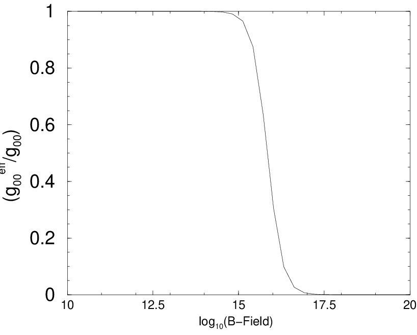
This effective metric corresponds to the result already derived in our previous paper (Mosquera Cuesta & Salim 2003;2004). We stress, meanwhile, that our former result was obtained by using the approximate Lagrangean
| (35) |
where , with , , , and was defined above. This Lagrangean is built up on the first two terms of the infinite series expansion associated with the Heisenberg-Euler (1936) Lagrangean, which proved to be valid for -field strengths near the quantum electrodynamics critical field G. In the present paper we overrun that limit. In fact, from Eq.(34) is straightforward to verify that the ratio , and goes all the way down to zero as the -field attains higher strength values. This means that the effective surface redshift grows unbounded as becomes larger and larger. Both results are displayed in Figs.1 and 2. Fig.2 also confirm that for canonical NSs the gravitational (GRS) redshift remains constant even for fields larger then the Schafroth QED limit.

4 Discussion and Conclusion
In a very interesting couple of Letters by Ibrahim et al. (2002;2003) was reported the discovery of cyclotron line resonance features in the source SGR 1806-20, said to be a candidate to a magnetar by Kouveliotou et al. (1998). The 5.0 keV feature discovered with Rossi XTE is strong, with an equivalent width of eV and a narrow width of less than 0.4 eV (Ibrahim et al. 2002;2003). When these features are interpreted in the context of accretion models one arrives to a M⊙ km-1, which is inconsistent with NSs, or that requires a low G magnetic field, which is said not to correspond to any SGRs (Ibrahim et al. 2003). In the magnetar scenario, meanwhile, the features are plausibly explanined as being ion-cyclotron resonances in an ultra strong -field G (see Eq.(1)). The spectral line is said to be consistent with a proton-cyclotron fundamental state whose energy and width are close to model predictions (Ibrahim et al. 2003). According to Ibrahim et al. (2003), the confirmation of this findings would allow to estimate the gravitational redshift (the GRS), mass () and radius () of the quoted “magnetar”: SGR 1806-20.
Although the quoted spectral line in Ibrahim et al. (2002;2003) is found to be a cyclotron resonance produced by protons in that high field, we alert on the possibility that it could also be due to NLED effects in the same super strong magnetic field of SGR 1806-20, as suggested by Eq.(34). If this were the case, no conclusive assertion on the ratio of the compact star glowing in SGR 1806-20 could be consistently made, since a NLED effect might well be emulating the standard gravitational one associated with the pulsar surface redshift.
In summary, because we started with a more general and exact Lagrangean, as that of Born & Infeld (1934), we can assert that the result here derived is inherently generic to any kind of nonlinear theory describing the electromagnetic interaction, and thus is universal in nature. Thence, absorption or emission lines from magnetars, if these stellar objects do exist in nature (see Pérez Martínez et al. 2003 for arguments contending their formation), cannot be saftely used as an unbiased source of information regarding the fundamental parameters of a NS pulsar such as its , or EOS.
Appendix
An additional outcome of the above procedure regards the modifications to the radial component of the background metric. For a pure radial -field the 4-vector unit can be written as
| (36) |
which renders
| (37) |
and consequently
| (38) |
Therefore, the third term in Eq.(32) reduces to
| (39) |
In this way, one can verify that such a radial-radial effective metric component is given by the relation
| (40) |
or equivalently
| (41) |
Some astrophysical consequences of this fundamental change in the radial component of the background metric will be explored in a forthcoming paper.
Acknowledgements
We are grateful to the anonymous referee for all the suggestions and criticisms that helped us to improve this manuscript. J. M. Salim acknowledges Conselho Nacional de Desenvolvimento Científico e Tecnológico (CNPq/Brazil) for the Grant No. 302334/2002-5. HJMC thanks Fundação de Amparo à Pesquisa do Estado de Rio de Janeiro (FAPERJ/ Brazil) for the Grant-in-Aid 151.684/2002.
References
- [] Born, M. and Infeld, L., (1934), Proc. Roy. Soc. Lond. A 144, 425
- [] Cottam, J., Paerels, F. and Mendez, M., 2002, Nature 420, 51
- [] De Lorenci, V. A., Klippert, R., Novello, M. & Salim, J. M., 2002, Phys Let B 482, 134
- [] Delphenich, D. H., 2003, report hep-th/0309108
- [] Glendenning, N. K., 1997, Compact stars: Nuclear physics, particle physics and general relativity, Springer-Verlag, New York, USA, p.390
- [] Hadamard, J., 1903, Leçons sur la propagation des ondes et les equations de l’Hydrodynamique (Hermann, Paris, 1903) Zeit. Phys.
- [] Ibrahim, A., et al., 2002, Astrophys. J. Lett. 574, L51
- [] Ibrahim, A., et al., 2003, Astrophys. J. Lett. 584, L17
- [] Kouveliotou, C., et al., 1998, Nature 393, 235
- [] Miller, C., 2002, Nature 420, 31
- [] Mosquera Cuesta, H. J., Salim, J. M., report astro-ph/0307519 (2003).
- [] Mosquera Cuesta, H. J., Salim, J. M., Astrophys. J. 608, 925 (2004).
- [] Mosquera Cuesta, H. J., de Freitas Pacheco, J. S., Salim, J. M., 2004, in preparation.
- [] Novello, M., De Lorenci, V. A., Salim, J. M., and Klippert, R., 2000, Phys. Rev. D 61, 045001
- [] Novello, M., Salim, J. M., 2001, Phys. Rev. D 63, 083511
- [] Pérez Martínez, A., Pérez Rojas, H., & Mosquera Cuesta, H., 2003, Eur. Phys. Journ. C, 29, 111. See also report hep-ph/0011399
- [] Sanwal, D., et al., 2002, Astrophys. J. Lett. 574, L61