Sensitivity as an Arbitrary Output Variable for Differentiable Rendering

Production renderers rarely output only the final picture. Alongside the beauty pass, an arbitrary output variable (AOV) exposes some intermediate quantity of the light transport, such as depth, surface normals, albedo, or object and material identity, so that artists can inspect, relight, denoise, and composite (Industrial Light & Magic, 2026). Decades of practice have made these outputs first-class: a compositor expects a normal pass, and an identity pass such as cryptomatte (Friedman and Jones, 2015) is a standard deliverable.

Differentiable renderers (Li et al., 2018; Nimier-David et al., 2019; Nimier-David et al., 2020; Vicini et al., 2021) expose a fundamentally new quantity: the derivative of any scalar objective evaluated on the image with respect to every scene parameter. A single reverse-mode pass returns, for each material, light, and geometric parameter, how sensitive the objective is to that parameter. To date this quantity has been consumed almost exclusively by optimizers, in inverse rendering and design. Yet the derivative is also informative on its own: it tells a human which parts of a scene matter for a given goal. Previous work (Beresna and Fiume, 2026) established that these gradients are interpretable and that the resulting rankings are objective-specific, but treated each map as a one-off visualization; what the quantity still lacks, and what is supplied here, is the output representation the primal image has long possessed, a reusable buffer and a taxonomy of the views read from it.

Treating the gradient of an output as an attribution over its inputs is by now standard in neural network interpretability (Selvaraju et al., 2017). We apply the principle to a different differentiable function: the inputs become scene parameters and the output an arbitrary scalar objective, so the attribution lands in the scene rather than in a feature map.

We propose the sensitivity AOV: a render output carrying the sensitivity of an objective to the scene parameters that influence it. Where a forward AOV is scene-intrinsic (depth is depth, independent of any goal), a sensitivity AOV is objective-conditioned, so the same scene yields different sensitivity AOVs under different objectives. Forward AOVs answer what is here; sensitivity AOVs answer what would change this.

Our contribution is a scaffolding rather than a single algorithm. We: (i) define the sensitivity AOV along four axes: selection, binding, aggregation, and encoding; (ii) observe that one reverse-mode pass populates a sensitivity buffer over the scene’s parameter hierarchy, from which many views follow without recomputation, in direct analogy to deferred shading; (iii) give a taxonomy of those views, distinguishing where a parameter lives from where its influence lands; and (iv) provide a reference implementation. Our aim is to establish derivative outputs as first-class render products alongside the primal image.

Let $\mathcal{R}$ be a differentiable renderer producing an image $I=\mathcal{R}(\boldsymbol{\theta})$ from scene parameters $\boldsymbol{\theta}$, and let $M$ be a scalar objective evaluated on $I$. A single reverse-mode pass yields

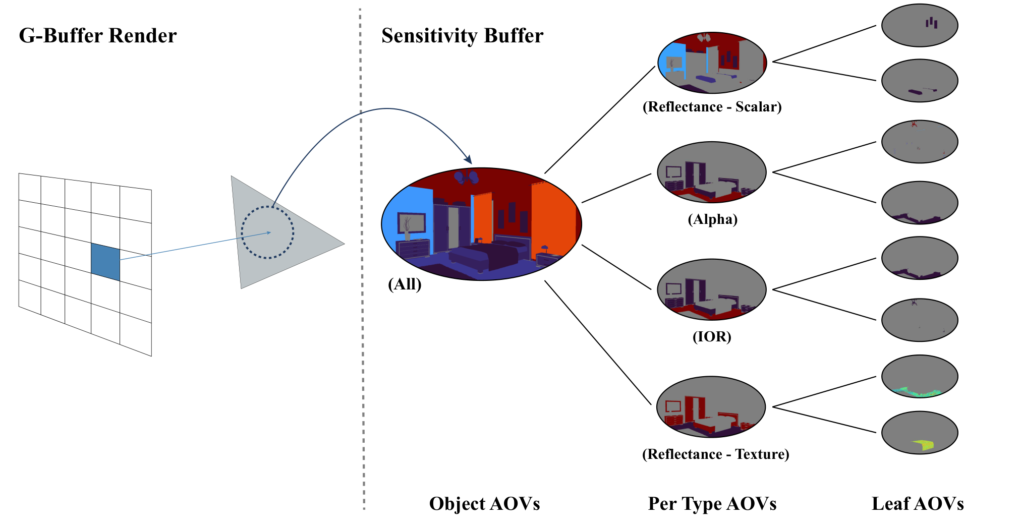
a vector assigning to every scene parameter a scalar sensitivity. Crucially, $\mathbf{g}$ is computed once, at the cost of one backward pass whose cost is largely independent of the number of parameters. We call the populated parameter set the sensitivity buffer. Every visualization we describe is a re-projection of this buffer, never a recomputation, the same relationship deferred shading has to the G-buffer (Saito and Takahashi, 1990): the adjoint sweep happens once, and the user then explores many views over the stored result.

Scene parameters are naturally hierarchical. Renderers expose them through structured keys such as floor.bsdf.reflectance, so the buffer is a tree: leaves are individual parameters, interior nodes are materials and objects.

The buffer of Section 2 is a tree of scalar sensitivities, one per parameter component. A sensitivity AOV is what results from reading that tree at a chosen granularity and drawing it: we select a subtree, aggregate its components to a single scalar per group, bind that scalar to pixels, and encode it for display. The first two steps decide what is shown, the last two where and how.

The buffer is a reverse-mode object: one objective propagated to every parameter at once, dense in parameters and sparse in objectives. Its transpose is forward mode, which pushes one chosen parameter through to every pixel, $\partial I/\partial\theta_{i}$. The two answer different questions, reverse for attribution (which parameters matter for this objective) and forward for prediction (what a single parameter does to the image), and the second cannot be assembled from the first without repeating the computation per parameter. Figure 5 places both side by side: forward mode is not an alternative to the buffer but its dual, suited to the question the buffer does not answer.

To keep the objective an example rather than a contribution, we use the simplest scalar on the image, its mean photometric response, $M=\tfrac{1}{|P|}\sum_{p\in P}Y(I_{p})$, where $Y(I_{p})$ is the photometric response of pixel $p$. We choose it because its sensitivities are easy to reason about, which makes the buffer and its views straightforward to check; the pipeline is agnostic to $M$, and a perceptual or learned objective enters at exactly the same point, changing only $\partial M/\partial I$.

Figure 1 shows the result on an interior scene. Read at the object level, the sensitivity AOV attributes the objective across the scene’s materials, including surfaces whose influence is carried by indirect transport and is not evident in the primal image. Read as per-type channels it separates which kind of parameter drives the objective, and the hierarchy would surface parameters such as a global exposure that never appear in the frame at all. The forward channels of Figure 5 and the free-viewpoint projection of Figure 6 come from this same single pass.

We realize sensitivity AOVs on a physically based path tracer with reverse-mode differentiation (Vicini et al., 2021; Jakob et al., 2022). Evaluating the objective and backpropagating populates the buffer via Equation 1, a single pass that all placement views then share. Binding a uniform parameter uses the object visible at each pixel, recovered from a one-sample-per-pixel primary-visibility pass that also yields the UVs and object identities the other views reuse. A spatially varying parameter carries its per-texel gradient to the surface through these UVs; because the gradient and the visible texel are sampled independently, we pool the per-texel field before projection to fill gaps and suppress fireflies, which is the main practical cost of the textured case. Hierarchy views are read directly from the tree and need no image-space pass at all. The forward-mode view is the one output not derived from the buffer: it requires its own forward-derivative evaluation, seeding a single parameter and propagating to the image, and is therefore recomputed per parameter shown. Everything else re-projects the one reverse pass.

The principal open view is the transport view: rather than painting a parameter where it lives, painting it where its influence lands, so that a wall’s reflectance colors the table it brightens through interreflection. Unlike the placement views, this cannot re-project a finished buffer: it must accumulate contributions during the adjoint sweep and is tied to a single viewpoint. We leave it, together with a fuller treatment of per-texel fields, which is the least explored case in our current implementation, to future work.

Several further limitations bound the present method. Our placement views read interior gradients and do not treat visibility discontinuities, so a boundary-correct account of geometric sensitivity is out of scope here. Sensitivities are local first-order quantities and do not capture interactions between parameters. Like all Monte Carlo derivatives they inherit path-tracing variance, so buffers computed at low sample counts may need denoising, and denoising a sensitivity field for faithful inspection, without reordering which parameters dominate, is itself an unstudied problem distinct from beauty-image denoising. Finally, our objectives are deliberately simple; richer perceptual and neural objectives fit the same framework and are natural to explore.

Differentiable renderers already compute, as a byproduct of every optimization, a quantity that answers which parts of a scene matter for a given goal. We have argued that this quantity deserves the same first-class output status as the primal image. The sensitivity AOV names the output, the sensitivity buffer reduces each further view to a primary-visibility pass over a stored result rather than a second adjoint sweep, and the selection, binding, and encoding choices determine how those derivatives are shown to a human. Forward AOVs describe what the scene is; sensitivity AOVs describe what would change it. Much of the space they open, the transport view, per-texel fields, denoising for human inspection, remains unexplored, and we offer this as scaffolding for it.