Vertex crossings in a symmetric Markov multinomial model
Abstract
We observe a ball bouncing down a Galton board with any number of directions. At each peg it either keeps its direction with some fixed probability or randomly turns to one of the other directions. Its bin measures how often it went each way, a point of a simplex. When the ball rarely turns, the most likely bins are the corners, which only a ball that never turns can reach. We ask when the best bin of each face of the simplex becomes as likely as a corner. To first order every face catches up at the same moment. We break this tie at second order, with an explicit constant for each face. Hence on a long board, as the expected number of turns grows to any fixed multiple of the length’s logarithm, the most likely bin jumps once, from the corners straight to the center. A nonuniform start or a weak external field changes the constants, potentially allowing an intermediate face to win.
Keywords: Potts chain; persistent random walk; Markov multinomial distribution; occupation counts; mode; spanning trees.
MSC2020: 60J10; 60F05; 60F10; 82B20; 05C05; 33C10.
1 Introduction
1.1 The question and the answer
Problem 131 of Kagey’s Open Problem Collection [1] is about a Galton board on which the ball tends to keep going the same way. At the first peg the ball goes left or right with probability , and at every later peg it repeats its previous direction with probability . Kagey asks when the middle bin is exactly as likely as the two end bins. Our companion paper [2], Paper A below, answers this for the persistent random walk, or Ising chain with free ends. It compares each bin with an explicit Bessel function, with an error bound that holds for every number of steps, and so traps the tie in an explicit interval for every board. Kagey also asks what changes on a tetrahedron. A natural version of that board sends the ball in one of three directions at each peg, and the bins after steps form a triangle, one layer of the tetrahedron.
Here we let the ball have directions. Its first direction is uniform, and at each later peg it keeps going the same way with probability (otherwise it turns to one of the other directions, each with probability ). After steps its bin is the vector of the numbers of steps in each direction. So the bins are the points of a simplex, a segment for and a triangle for . Only a ball that never turns reaches a corner , or vertex, so each vertex has probability .
When is close to the ball rarely turns, and the vertices are the most likely bins. As decreases the other bins catch up. On the triangle there are two natural candidates to catch up first, the middle of an edge, where the ball has used two directions, and the middle of the triangle, where it has used all three. We ask which one wins, and when.
Put and . To first order every face of the simplex catches up with the vertices at the same place, namely when is about . So the first order cannot answer the question. We break this tie at second order, and the center of the whole simplex wins. For large , as grows from to any fixed multiple of , the most likely bin jumps once, from the vertices straight to the center, and no edge or other proper face holds it in between. On the triangle the middle bin overtakes the corners while the middles of the edges are still about below them. Figure 1 shows this at .
Why every face ties.
Take a face with directions. A ball that uses only these directions must avoid the other directions at every peg, and it does so with probability . So the face carries mass about , while a vertex carries . On the face the ball turns about times toward each direction, so the fractions fluctuate by about around . So the mass of the face is spread over about bins near its center, and
The bracket is the same for every face, and it crosses when . Only the constant in front can tell the faces apart.
How second order breaks the tie.
The constant is , the mass of the face over the Gaussian volume of the fluctuations, whose covariance is (Proposition 3.7). So the ratio is with the common bracket , which increases as decreases. Since , the full face reaches the vertices first, when , while a face with directions is still below them by the factor . On the triangle this factor is . After that moment the full center beats every proper face, since when .
1.2 Setting and notation
Fix and a start law on the set of directions, which we also call states. Let be the Markov chain with that keeps its state with probability and moves to each of the other states with probability . Put . Kagey’s board is with the uniform start.
Bins. The count vector records how often each state occurs among . A bin is a vector of nonnegative integers with sum , and . For the uniform start we write . The uniform start is the default everywhere except in Section 4.
Faces and vertices. A face is a nonempty set , and . A bin lies on the face . The vertices are the faces of size , that is, the bins . A word that reaches never switches, so , and for the uniform start we write .
Balanced bins. A bin with positive coordinates is balanced if these coordinates differ by at most . For the uniform start all balanced bins with positive coordinates have the same probability, since they differ only by a permutation of the states. We call it , so .
Scales. Put and . The expected number of switches (turns) is , so is about the expected number of switches to each other state. Put . For let , the odds of a switch to one given state against no switch, and . For we have and also use . Since , the scales and differ by when . This is smaller than every error term in our asymptotic statements, so these statements hold with either one. Exact statements are written in .
Crossings. For , the crossing is the value of at which , and is the value of there. We write when the number of states matters.
The constants. For put
| (1) |
Numerically , and .
Matrix form. The transition matrix is with , where is the all-ones matrix, so switches at rate to each other state. The exit rate of a face with states is , the principal Dirichlet eigenvalue of on .
Potts chain. With the uniform start and , a word has probability . This is the one-dimensional -state Potts model with free boundaries. For it is the Ising chain of Paper A.
Asymptotic notation. In each statement the constants in , and the threshold behind “for large ”, depend only on the quantities declared fixed in that statement (always including and ). Uniformity in the other variables is stated each time.
1.3 Main results
Theorem 3.1 makes the heuristic of Section 1.1 precise. Uniformly for , the logarithm of is , up to a next term that is again proportional to and an error . Part (ii) of that theorem is the first-order statement. With , a balanced bin on a face has probability . At the exponent equals for every face, so the first order cannot choose.
By Theorem 3.2, for every the balanced bin with positive coordinates crosses the vertices at exactly one , which increases with , and
| (2) |
For the model is the persistent random walk of Paper A. For equation (2) is the crossing equation of Paper A [2, Proposition 3.8], and is its constant . Since , Corollary 3.9 shows that for large and all the global mode changes exactly once, from the vertices straight to the balanced bins with positive coordinates. All the face-center crossings lie in a -interval of length . For small this can fail. On the triangle with an edge center can be the mode (Example 3.10).
The same method gives the crossing of every bin whose positive coordinates are of order (Theorem 3.3). For fractions its constant is with , where is the occupation covariance of a tilted chain, and is a weighted count of the spanning trees of the complete graph (Proposition 3.6). At the center the count is Cayley’s , and .
Then we perturb the model in two ways. Each acts at order , namely the order of the constants . A start law changes the constant of a face against a vertex to (Theorem 4.4). The best bin of each face keeps the share of the uniform value (Theorem 4.6), so each face gets a line in and the highest line holds the mode (Corollary 4.7). On the triangle with this lets an edge hold the mode on a window of width in (Example 4.9). A Potts field of size per visit to state adds to each face the field averaged over the face (Theorem 5.2), and one field makes every support size win in turn (Corollary 5.4).
Finally we drop the assumption that the positive coordinates are of order . A Bessel majorant has relative error for every positive count vector when (Theorem 6.2). When at least two coordinates are of order , a small coordinate starts to matter once it has size (Theorem C.1). Near a vertex, with one large count and small counts of total , the crossing odds are , where is the root of a product of Laguerre polynomials (Theorem 6.4).
1.4 Related work
The law belongs to the theory of Markov multinomial distributions. Edwards [4] introduced the Markov binomial distribution. Let be a law on the two outcomes of a trial, success and failure. His trials form a stationary chain with law at each trial that moves from to with probability . He wrote the generating function of the number of successes as a product of matrices. Wang and Yang [3] extended this chain to finitely many states. We have not seen their paper, and we describe it through Johnson, Kotz and Balakrishnan [5, Chapter 35, Section 13.2]. The chain of Wang and Yang starts from a law and moves from to with probability , where , and the generating function of its vector of category counts is a product of matrices. Our chain with the uniform start and is the case where is uniform and . So the exact law for the uniform start is a special case of this theory, and we do not claim it as new. Our general start changes only the initial law and keeps the uniform switching, so it is a Wang–Yang chain only when is uniform. Hsiau [7, Theorem 1] proves compound Poisson limits for sums over multistate chains with one nearly absorbing state, and Wang and Tang [6] prove Poisson-type limits for additive processes on Markov chains. Whittle [8, formula (8)] gave the exact law of the transition counts of a finite chain. The count vector is determined by the transition counts and the first state, so could also be summed from his formula.
Brydges, van der Hofstad and König [9] give occupation densities for continuous-time chains on the visited faces of the simplex. Huang, Kious, Sidoravicius and Tarrés [10, Theorem 1] give the joint density of the local times, the last-exit spanning tree and the net crossing numbers of a walk with symmetric conductances, with Bessel functions. Stadje [11, Theorems 1 and 2] gives the generating functions of the joint numbers of visits of a finite chain. He also proves limit laws when one state becomes nearly absorbing and the chain leaves it with probability of order [11, Theorems 3 and 4]. The other rows of his transition matrix stay fixed, so the counts of the other states stay bounded. Dietz and Sethuraman [12] study chains that switch from to at time with probability . They make about switches by time , but only of them after time , and their occupation fractions have a limit law on the simplex. Our chain makes about switches near the crossings, spread evenly in time. Dupuis and Liu [13] give the rate function of the occupation measure, which we compare with our exponent in Section 3. Kassan-Ogly and Filippov [14] solve the Potts chain in a field in the thermodynamic limit. Their paper was not accessible to us through standard means or institutional libraries, but its abstract and introduction are free online, and we use nothing beyond these. Aside from this, no source we could read compares one count vector with a vertex when depends on , and none of them finds the face-center crossings or the tie. We take the Bessel and Laguerre formulas from [16].
2 The model and the exact law
We write in three forms. The run form counts the switches, and it gives all our exact statements. The refresh form uses the transition matrix . When the chain keeps its state with probability and otherwise draws a fresh state uniformly from all states, possibly the same one. The ratio form is the refresh form divided by a vertex (so it measures a bin in units of a corner). For it is a sum of positive terms, and all our asymptotics start from it.
For a positive count vector with total and a state , let be the number of words with counts and changes that start with , and let . Put
These polynomials do not depend on . For a bin with some zero coordinates, and mean the polynomials of its positive coordinates.
Proposition 2.1 (the generating function).
Put and . As formal power series,
Proof.
Let be the generating function of the words of length at least that end in state , each weighted by its probability, and let . Conditioning on the last letter gives , that is, . Summing over gives , and the generating function is . ∎
Proposition 2.2 (the exact law).
Let , let be a bin, and put . Sums over run over the integer vectors with for and for , and .
- 1.
(refresh form) With ,
For the uniform start this reads
- 2.
(run form) If , then . In particular .
- 3.
(ratio form) If , so that and , then
(3) which is a sum of positive terms.
When , the refresh form has a direct reading. Cut the word into blocks at the refreshes. Each refresh lands on a prescribed state with probability , and each of the other steps keeps the state with probability . If blocks carry state , there are orders of the block labels that start with , and ways to choose the lengths of the blocks of state . The proof below does not need .
Proof.
(a) By the proof of Proposition 2.1, . By the multinomial theorem the coefficient of in is . With we have , and for . For only contributes. Multiplying the coefficients proves (a), and for the uniform start .
(b) A word that starts with and has changes has probability . Sum over the words with counts .
(c) Divide the uniform case of (a) by . Since and , we have . ∎
At we have and only survives, which gives the multinomial law for the uniform start. At only survives, which gives mass at . For the terms in (a) can cancel, so for numerical work we then use exact arithmetic or dynamic programming.
2.1 Bessel bounds
For the modified Bessel function of order is . Since , comparing coefficients gives . We also use the expansion [16, Eqs. 10.40.1 and 10.17.1]
and the function
Since , we have , and comparing term by term with the even part of the series of gives . Lemmas A.1, A.2 and A.3 in Appendix A give the other facts about that we use.
3 The tie and its resolution
In this section the start is uniform. The constants , and are those of (1). Let be a balanced vector with positive coordinates and total . By Proposition 2.2(b), , and as a function of this ratio does not depend on .
3.1 Every face ties at first order
Theorem 3.1 (every face ties at first order).
Fix and .
- 1.
For large , uniformly for and ,
- 2.
Put . Uniformly for and , a face with states has
At the right side is for every .
- 3.
Put . Uniformly for in a compact interval, for each ,
(4) - 4.
.
So the central bin of every face reaches the vertices when , and by (iii) the faces differ in this window only through the constants .
Theorem 3.2 (face-center crossings).
For every and there is exactly one with . The balanced bin is more likely than a vertex below and less likely above it. The crossing is strictly increasing in ,
and every crossing has , so . For fixed the value of at the crossing satisfies
and
| (5) |
For , is the crossing of Paper A [2, Section 3.2], is its constant , and (5) is its third-order expansion [2, Corollary 3.7(c)]. The proofs here do not use the binary case. Figure 1 shows the full-center crossing on the triangle at .
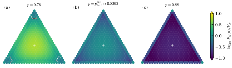
Idea of the proofs.
The proofs are in Appendix A. The exact part uses the run form. The polynomial has nonnegative coefficients, and its first nonzero coefficient is , from the words that use each state in a single run. So increases from to and crosses exactly once. Its next coefficient grows with , which moves the root. The asymptotic part uses the ratio form (3). This sum is close to a Bessel integral (Theorem 6.2), and the Laplace expansion of this integral (Lemma A.4) gives, for a balanced with positive coordinates and uniformly for ,
| (6) |
This is the heuristic of Section 1.1 with the constants made explicit. Then and give parts (i) to (iii) and the expansions of the crossing. Part (iv) follows from the monotonicity of .
3.2 The constants as Gaussian volumes
By the heuristic of Section 1.1, should be the mass of a face divided by the Gaussian volume of the fluctuations of the fractions. We prove this in two ways, namely at each interior point of a face (Proposition 3.6) and by a sum over the whole face (Proposition 3.7). The next theorem evaluates its constants at the actual fractions , since we do not assume that the count vector converges at any rate.
Theorem 3.3 (interior compositions).
Fix , and . Let with , and put
Uniformly for these count vectors and ,
| (7) |
The unique positive root of satisfies
| (8) |
For a fixed target and counts , the constants may be evaluated at the target without changing the error order.
So a bin with fractions grows like against a vertex and crosses at . By Cauchy–Schwarz , with equality only at the center, where . Since , both displays also hold with in place of and of .
The exponent is a drop in a rate function (the cost of holding the fractions near ). By Dupuis and Liu [13, Eq. (3.2)], the occupation measure of the chain with generator has rate function . So , the drop in the rate from a vertex to . The next lemma computes the determinant of an occupation covariance for any reversible chain.
Lemma 3.4 (occupation covariance).
Let be an irreducible generator on , reversible with respect to , with conductances for . For let , and let solve with . Let be the matrix of the quadratic form on the vectors with , in the coordinates . Let be the Laplacian without its first row and column. Then
where the sum is over the spanning trees of the complete graph on .
The form is the usual asymptotic variance per unit time of for the chain with generator , but we use it only as a definition. The proof is in Appendix A. For product conductances the tree sum has a closed form. This is classical, and we include a short proof.
Lemma 3.5 (weighted Cayley formula).
For and conductances ,
With every this is Cayley’s count of the spanning trees of .
Proof.
Put . The Laplacian is , so with . The matrix determinant lemma gives , and this is by the matrix-tree theorem. For integer conductances this is the multigraph case [15], and both sides are polynomials in the . ∎
Proposition 3.6 (the tree form of the constants).
Fix and in the open simplex. Put entrywise and .
- 1.
The chain with rates for is reversible with stationary law and conductances . Let and entrywise. Then is symmetric with Perron root and Perron vector , and is its Doob transform . It is not a Doob transform of itself unless is uniform.
- 2.
.
- 3.
- 4.
At the center , each of the spanning trees has weight , and . In the coordinates , with and of size , and . So
- 5.
The same holds for the constant of Theorem C.1, with and in place of and .
The proof is a direct check, given in Appendix A. The second way sums the whole face. Its total mass is explicit, and comparing it with the Gaussian sum of the interior profile gives again.
Proposition 3.7 (mass balance).
Fix , and let the sums run over the positive vectors with .
- 1.
For every and every ,
- 2.
For fixed , uniformly for and , this sum is , and it is also .
- 3.
Hence .
Proof of (1).
A word of length over a set of letters with exactly changes is fixed by its first letter, the positions of the changes and the new letter at each change. So there are of them. By inclusion and exclusion over the set of allowed letters, the number of such words that use all letters is , and this is . Multiply by and sum over . ∎
Parts (2) and (3) are proved in Appendix A. The term in (1) is for a face with states. So is the mass of the face, in units of a vertex, divided by the Gaussian volume of the occupation fluctuations. This is an interpretation, not an independent derivation of , since part (2) uses Theorem 3.3 near the center.
3.3 Balanced bins and the global mode
So far we have compared balanced bins with vertices. To find the global mode we also need that the balanced bins are the best bins of their face.
Theorem 3.8 (balancing within a support).
For , among bins with a prescribed set of positive coordinates and total , the probability is largest exactly at the balanced bins. More precisely, moving one unit from a coordinate to another coordinate , where and , strictly increases the probability of the bin.
Once the number of runs of each state is fixed, splitting the visits evenly gives the most ways to choose the run lengths. In the proof in Appendix A this becomes the log-concavity in of the polynomials of (17). The condition holds at every crossing, by Theorem 3.2.
Corollary 3.9 (exactly one mode change).
Fix and . There is such that for and every with the following hold.
- 1.
If , the global modes are exactly the vertices.
- 2.
If , they are exactly the balanced bins with positive coordinates.
- 3.
If , they are these two classes and nothing else.
Moreover and . So all face-center crossings lie in a -interval of length , and as decreases the full center crosses first.
By Theorem 3.8 every global mode is a vertex or a balanced bin, and Theorem 3.1(i) compares these as in Section 1.1. The proof is in Appendix A.
Example 3.10 (an intermediate face can be a finite-size mode).
4 A general start
Suppose now that the ball starts in state with probability , and moves as before. The start affects only the first run (the steps before the first turn), but it changes the constants by an amount of order , the order at which the faces are separated. So a start can decide which face wins.
For a count vector with support , Proposition 2.2(b) gives
So the start enters only through the weights , which sum to . A vertex has . Throughout this section, is a face with states and (if , every bin with support has probability ), and is a vertex with .
Lemma 4.1 (start weights).
Let be a positive count vector on .
- 1.
If , then . So for all when is balanced and divides .
- 2.
Fix . There are and , depending only on , and , such that for , and every balanced bin of ,
So a balanced bin forgets where the path started, up to a relative error . The proof is in Appendix B. For other bins we look at the first run of the path.
Lemma 4.2 (the first run).
Let be a positive count vector on and let . Then, as polynomials in ,
Here is the polynomial of the positive coordinates of , and it equals when .
Proof.
A word with changes has weight in . Note that with , since and for . Expand every factor into its two terms. The term with no is nonzero only for a constant word, and a word that uses states is not constant. For a word that starts with and a nonzero term of its expansion, let be the first step at which the term is chosen. The steps before give , so and . Step gives , whatever is. The later factors, summed over their terms, give the weight of the word , which can be any word with counts . Summing over these words gives . ∎
In the refresh reading of Section 2, the path stays in until its first refresh, and after it the path no longer depends on where it started.
Proposition 4.3 (where a conditioned path starts).
Fix and , and put and . Uniformly for positive count vectors on with every , for and for ,
Under the uniform start, is the probability that the chain starts in given . So a path conditioned to have fractions starts in with probability close to rather than . Note that is the Perron vector of Proposition 3.6. The proof is in Appendix B. By Lemma 4.2 and Theorem 3.3, removing visits from lowers by a factor of about , and the sum over gives . For , , and the error is , about (numerically verified, see Section 7).
Theorem 4.4 (face-center crossings with a start).
Let be a balanced bin of .
- 1.
For every , the ratio is a polynomial in with nonnegative coefficients, zero constant term and lowest term . So it equals at exactly one , and the bin is more likely than the vertex below this . If divides , then . So the crossing solves , its decreases strictly along , and at it is .
- 2.
Fix and let be as in Lemma 4.1(2). For , uniformly for and over all , .
- 3.
Put . Fix . For large , uniformly for and over all ,
Fix also . Uniformly over the with , the value of at the crossing of (1) satisfies and the expansion (5) with in place of , and with the ratio tends to , uniformly for in compact sets. Here the constants depend also on .
Note that a start changes only the constant of each crossing. It lowers by , the logarithm of the average start weight on the face against the start weight of the vertex, shared among the new states. When does not divide the crossing can depend on the balanced bin , which is why we write .
Proof.
(1) Each has nonnegative coefficients, zero constant term and lowest term , from the orders of the states that start with , with each state in a single run. So the ratio increases strictly from to in , and decreases from to on . If divides , Lemma 4.1(1) gives . The rest of (1) is about , which increases strictly along at every and equals at , by the proof of the exact part of Theorem 3.2.
(2) is Lemma 4.1(2), divided by .
If is constant on , say for , then for every with support in . So the statements of Sections 3 and 6 about such bins hold verbatim, with replaced by for a vertex . In particular Theorem 3.8 holds on . Otherwise balancing can fail.
Example 4.5 (balancing can fail).
Let , and with . Counting the changes in the four words with counts and the six with counts gives and . So , and the unbalanced bin is more likely when .
By Theorem 4.4(2), a balanced bin of has the share of , up to a factor . The next theorem shows that no bin of , balanced or not, does better by more than a factor .
Theorem 4.6 (face maxima with a start).
Let be a face with states.
- 1.
Fix . For large , uniformly for and over all with ,
So with , uniformly for in compact sets and over all such ,
- 2.
For with support put . Fix a compact set of and . For large , uniformly for and over all with , every bin that maximizes among the bins with support has .
So a start can move the best bin of away from the balanced bins, but it gains at most a factor , and in the window the best bin stays within of the center. The bound holds for every bin of , including bins with coordinates that are . The proof is in Appendix B, and it rests on Lemma 4.2. By Theorem 3.8, each is at most the balanced value at total , which is about times the balanced value at total . So is at most about times the balanced value, and is the start weight of each state at a balanced bin.
Each face now gets a line in the window coordinate , and the highest line wins.
Corollary 4.7 (global modes with a start).
Order the start weights as , put and , and define the lines
Fix a compact set of on which is attained only at . For large and all , every global mode of has exactly positive coordinates, and its support has . If , the global modes are exactly the vertices with . If and is constant on such a support , every global mode with support is a balanced bin, and all balanced bins of have the same probability. If , then for every fixed and large , every global mode has for each in its support.
The proof is in Appendix B.
Remark 4.8 (the order of the winners).
The winning size is nondecreasing in . Indeed, if attains at and attains it at , adding the two inequalities and gives . Put , where and cross. Since the slope of lies strictly between the slopes and , a size can be the unique winner at some only if . For the uniform start and , in line with Corollary 3.9.
Example 4.9 (the start decides which face wins).
Let and , and put . Fix and let be large. If , the global modes are and . If , they are exactly the balanced bins of the edge . If , every global mode has three positive coordinates. The window has width , while with the uniform start no proper face wins (Corollary 3.9).
Proof.
Here and , so the lines of Corollary 4.7 are , and . Hence exactly when , exactly when , and exactly when , where , which is the point of Remark 4.8. By (1), . This is positive, since . Also . So , and the unique winning size is for , for and for . Now apply Corollary 4.7 with . The vertices with are and . The only edge with is , and is constant on it. So for every global mode is a balanced bin of . Hence the global maximum equals the maximum over the bins with support , and since all balanced bins of this edge have the same probability, each of them attains it. ∎
Dynamic programs over all bins at , and show the three phases at finite , with the window moved to larger (numerically verified, see Section 7). The next remark explains the shift.
Remark 4.10 (the window at finite ).
Let be the unique positive root of , which is the crossing odds of Paper A [2, Theorem 3.1]. Since is constant on , we have , so for every the balanced bins of the edge cross the vertices exactly at , that is, at . This differs from Paper A’s by . Near the lines of the full face and of the edges through stay below those of the vertices, so for large this crossing is the lower end of the window. For the two ends at finite we use . A heuristic calculation, which we do not prove, puts them at and . Only is proved, by Theorem 3.2. The terms come from a discrete term in the logarithm of (6). Exact computations give the widths , , and at , , and , and the heuristic gives , , and (numerically verified, see Section 7).
5 A weak Potts field as a tilt
In this section the start is uniform again. Give each visit to state the extra weight , for a fixed vector . Over steps these weights multiply to , a factor of order , which is the scale of the constants . So the field can reorder the faces. We study the tilted occupation law
| (9) |
We use the window coordinate . The normalizing sum cancels whenever we compare two bins. A modal phase is the support of the global modes, which need not be the face with most of the mass.
Proposition 5.1 (the field is a tilt).
Let .
- 1.
. So is the exponential tilt of the law of the occupation rate by the linear function .
- 2.
It is also the law of the counts when the law of the path is tilted by . This is the Potts chain with free boundaries, coupling per equal neighbor pair and field at each site.
- 3.
If , then .
Proof.
Part (1) is (9) with its denominator written as . For (2), a word has probability , and depends on the word only through its counts . So tilting the words and then counting gives (1).
For (3), the chain is stationary with transition matrix , whose -th power is . So , and the indicators of state at times and have covariance . Summing over the two times gives, for ,
We bound this in two cases. Note that . If , then , the second term in the bracket is not positive, and . If , then , the bracket is at most , and , so . In both cases tends to the uniform vector in probability as . Since is bounded, bounded convergence gives the limit. ∎
By (1), for every . This is of the order of the constants , but invisible at first order, so a field of total size does not change the exponents of Theorem 3.1(ii). For a support with put .
Theorem 5.2 (weak-field modal phase diagram).
Put and define the face scores
The largest bin weight, taken relative to the untilted vertex and before the normalization in (9), satisfies, uniformly for in compact sets,
| (10) |
For fixed and all large , every global mode has a support that maximizes the limiting score. If the maximizing support is unique, all global modes have exactly that support. On a selected support with , their locations satisfy
This does not identify the maximizing vectors exactly, and equal limiting scores do not imply that both supports hold modes at finite .
If the fields are sorted as , the maximum of the scores is the upper envelope of the lines
| (11) |
Away from ties, the winning support size is nondecreasing in . If the fields are strictly ordered, the winning supports are the nested sets . Every support size is the unique winning size on an open interval of for suitable fixed fields. So proper-face phases persist under a field of order per step.
So the field shifts the line of each face by the field averaged over the face. The reason is that on a support the ratio of a bin to a vertex has a Gaussian profile of width around the center of the face (Lemma B.1), where the tilt is . The proof is in Appendix B.
Example 5.3 (a persistent triangular edge phase).
For and the three competing scores are , and . If , the edge wins strictly for
and for every fixed in this interval all global modes of the tilted law lie on that edge for large . Without a field no proper face holds a mode in the window (Corollary 3.9).
One field can make every support size win in turn, from one state to all .
Corollary 5.4 (one field realizes the full face hierarchy).
Fix and , and let for . In particular works in every fixed dimension. Put
and , . Then , and for every the support is the unique winning support on the nonempty interval . So for each fixed in this interval and all large , every global mode of the tilted law has exactly those positive coordinates.
6 Near the boundary of the simplex
So far every positive coordinate was of order (Theorem 3.3 needs each to be at least ). In this section we no longer assume this, and first give an upper bound that holds for every positive count vector (Theorem 6.2). Then we find the scale at which a small coordinate starts to matter. It is when at least two coordinates are of order (Remark 6.3). Near a vertex the crossing moves to odds of order , and the small coordinates alone decide it (Subsection 6.1).
The start is uniform, but does not involve the start, and Proposition 2.2 gives . So every upper bound below also holds for a general start.
Lemma 6.1 (a uniform Laguerre–Bessel inequality).
For every integer and real ,
| (12) |
By [16, Eq. 18.5.12], with the Laguerre polynomial , so the lemma is a quantitative form of the limit of Laguerre polynomials to Bessel functions. The proof, in Appendix C, compares coefficients with Lemma A.2.
Theorem 6.2 (a uniform Bessel majorant on every simplex stratum).
Let be arbitrary positive integers with sum , and let , . Define
Then, with no lower bound on any ,
| (13) |
So this approximation has relative error whenever , uniformly over every positive composition of .
For the central bin of the segment, is a bound of the same kind as the uniform Bessel bound of Paper A [2, Theorem 3.3]. The proof is in Appendix C. It applies Lemma 6.1 to each factor of an integral form of , and an integration by parts bounds the resulting mean.
Remark 6.3 (the scale ).
A small coordinate adds its own runs. Each run needs about two switches, which gives a factor , and it can go in about places. So what matters is . At the crossings of Section 3 the value is of order , and then is of order . So when at least two coordinates are of order , a rare count starts to matter once it has size with fixed.
Appendix C proves this. Take large coordinates with fractions among themselves and rare counts . With , Theorem C.1 gives up to a factor . Each rare count contributes a factor , where , and the complete correction of relative order is a factor with three terms. The theorem also gives the crossing as the root of an implicit equation, and as an explicit expansion in , which converges slowly. Rare counts with change that expansion only by (Corollary C.3). With only one large coordinate the growth factor is gone, since . Then the crossing moves to of order , where is the large count. This is the case of Subsection 6.1.
6.1 Near a vertex
Now let one count be large and let the other positive counts be small compared with , with fixed. In this subsection and in Appendix D we put . These rare counts are not the constants of Section 3, which do not appear here. With as in Lemma 6.1, put
The polynomial has positive coefficients, and , so has exactly one positive root , and . Write for with . It is a polynomial in with nonnegative coefficients, zero constant term and a positive coefficient at , so has exactly one positive root .
Each rare run again needs about two switches and has about places, so the rare counts enter through . For fixed rare counts the bounds of Lemma D.2 give as . So the crossing is near , and is of order instead of . The next theorem shows that this stays correct uniformly as long as .
Theorem 6.4 (all growing rare counts near a vertex).
Fix and put
For all positive counts with ,
| (14) |
In particular
| (15) |
so as . The constants are not optimized.
The proof is in Appendix D. It rests on two facts. First, is concave, and for its elasticity lies between and (Lemma D.1). Second, exactly, where and is a gamma variable plus a compound binomial sum with mean (Lemma D.2). Jensen’s inequality then gives , which exceeds at . The tangent line of at and the moment generating function of give an upper bound that is below at .
7 Verification and open questions
Data and code availability.
No proof in this paper relies on computation. The code and the Lean files are in the folder kagey-problems/problem131 of https://github.com/apemm/Kagey-Problems (release paperB-arxiv-v1). The checks for this paper are described in SUPPLEMENT.md. The scripts are in the subfolder paperB and use only the Python standard library. The command python -B verify_all.py --paper b in kagey-problems/problem131 runs all of them except verify_B_tie_repair.py, which also runs when --full is added. The scripts compare the exact law with dynamic programs and with enumeration of all words, and check the crossings and the constants. The statements marked as numerically verified are checked as follows. For the error quoted after Proposition 4.3, verify_general_start.py computes the start weights from the run form and from the refresh form in double precision. For the finite- phases after Example 4.9, dynamic programs over all bins run at in verify_general_start.py and at and in verify_B_tie_repair.py. For Remark 4.10 the two ends of the window are found by bisection, at in verify_B_tie_repair.py and at in verify_general_start.py. The scripts verify_frontier_modes.py, verify_frontier_boundary.py and verify_vertex_completion.py check the field and the identities near the boundary against word enumeration. The numbers in Remark C.2 come from verify_crossover_factor.py. For it computes in three ways, by the run form and by a quadrature of (21) in double precision and by the sum (3) in 60-digit decimal arithmetic, and for larger by the last two. They agree to about in . None of these checks is interval-certified.
Many of the exact identities and finite bounds were also formalized in Lean 4, in kagey-problems/problem131/lean/PaperB, where MAP.md matches each statement with its Lean theorem. These include the exact law for the uniform start, balancing, the ordering of the constants , most of the arithmetic of Corollary 5.4, and the bracket near a vertex. The asymptotic results and the results for a nonuniform start were not formalized.
Open questions.
Several questions remain open. The discrete correction term and the second-order ends of the window in Remark 4.10 are not proved. Neither is the failure of balancing at every large for a start that is not constant on the face. Corollary 3.9 has no effective , and by Example 3.10 it does not extend to every . Nothing is said here about the modes when is much larger than . Near a vertex the leading crossing is known uniformly for rare counts of total , but neither the next term uniformly in that range nor the case of a nonuniform start is known. The crossover with a start that is not constant on the support, and a number of states that grows with , are also left open. Switching that is not uniform is treated in a paper of the author that is in preparation.
Acknowledgments.
I thank Peter Kagey for posing the problem, and Chase Hameetman and Aidan Deshong for insightful conversations about some of the proofs in this paper.
A note on the use of AI
I wrote the proofs and derivations of Sections 2 and 3 by hand, without AI assistance, before any revision. I then used Claude Opus 5.5 (Anthropic, through Claude Code) in September and October 2026 to check everything I had written for typos and for statements that were technically wrong. It found a number of gaps, which I fixed, along with occasional wrong references and unclear wording. I decided every revision and went over each one by hand. The model also drafted rewordings of many passages, which I reviewed and edited. For the later sections I brainstormed conjectures with the model, and several results came from it together with proofs, namely the tree form of the constants in Proposition 3.6, the start-law results (Lemma 4.2, Proposition 4.3, Theorem 4.6, Corollary 4.7 and Example 4.9) and the full correction factor in Theorem C.1. I rechecked and rederived these proofs by hand. I also checked the proofs with GPT-6 Astra (OpenAI), which found nothing beyond the earlier check.
The Lean 4 formalization in kagey-problems/problem131/lean/PaperB was generated by the model, then revised and checked by hand against the corresponding results (see MAP.md in that folder). Parts of the Python verification scripts were also written by the model, which cross-checked them against each other. Lastly, I used it for literature search, namely to find and verify sources beyond the ones I had first checked on my own.
All mathematical claims, proofs and computations in this paper are my responsibility.
Statements and declarations
Competing interests.
The author has no competing interests to declare.
Funding.
No funding was received for this work.
Data availability.
All code, data and Lean files supporting this paper are in the folder kagey-problems/problem131 of https://github.com/apemm/Kagey-Problems, at the release paperB-arxiv-v1. Section 7 describes what each check does and how to rerun it.
Appendix A Proofs for Sections 2 and 3
A.1 Facts about Bessel series
The weights of the series define a probability law on the integers . Its moments control every Laplace expansion in this paper.
Lemma A.1 (the Bessel law).
For let be a random variable with for (so when ), and put . Then
- 1.
,
- 2.
,
- 3.
, and for ,
- 4.
, so for , and ,
- 5.
,
- 6.
for .
Proof.
(i) We have . (ii) For , and , so the sum is . (iii) The first form is the definition of the mean. Termwise, by the series of [16, Eq. 10.25.2], which gives the second. (iv) Since plus a term free of , we have . So , and . From the series, , so . (v) For integers we have , so by (i). Also . (vi) follows from (iii) and (v). ∎
Lemma A.2 (clipped product deficit).
For any finite list of nonnegative real numbers , with ,
Proof.
If some , the product is zero and the sum is at least one. Otherwise all factors lie in , and induction on follows from for . The empty product gives equality. ∎
Lemma A.3 (Gaussian averages of the factors ).
Fix , an integer and . Let and with , and put . Let be independent, with distributed as in Lemma A.1 with . Put and . Then
and for . The constants depend only on , and . Moreover
Proof.
Step 1. Derivatives as moments. Expanding each gives , where runs over vectors of nonnegative integers, and . The weights are the joint law of . Hence , where . In particular .
Step 2. The fourth derivative. Let with . For every we have (consider and separately) and . Applying this with termwise gives
where the are independent with the parameters in place of . By Lemma A.1(i) and (ii), . Hence is bounded in terms of , and . Since we have , so . The same argument without derivatives bounds .
Step 3. Taylor expansion. Expand to third order in with the Lagrange remainder. The odd terms integrate to zero over the symmetric interval. The integrals of and over differ from and by , the number is bounded, and the remainder term is . This proves the expansion.
Step 4. The formula for . Put . Then by Lemma A.1(i), and independence gives . Subtracting proves it. ∎
A.2 Proofs for Section 3
Proof of the exact assertions in Theorem 3.2.
Let be a balanced vector with positive coordinates, so that with .
Step 1. One crossing. To count , choose a sequence of run colors in which successive colors differ. If color appears times, its run lengths can be chosen in ways. So every coefficient of is nonnegative, and the first nonzero one is , from the orders of single runs. Hence increases strictly from to on and equals exactly once. As increases over , decreases over , which gives the unique and the two inequalities.
Step 2. Monotonicity in . Choose the balanced vectors for increasing by adding to one of the smallest coordinates. Each coefficient is then nondecreasing. To see this, map a word to the word with an extra copy of the incremented color just before its first occurrence. This keeps the number of changes, and it is injective, since deleting the first letter of the first run of that color inverts it. The coefficient of is
To see this, note that exactly one run color appears twice. For each choice of it there are sequences of run colors in which successive colors differ (all orders, minus those with the two copies adjacent), and ways to split its visits into two runs. This coefficient increases strictly with . So at every the value increases strictly with , the root of decreases strictly with , and increases.
Step 3. The first crossing. If , every coordinate is and , which gives . Since the root decreases with , every root has , and means , that is, . ∎
The asymptotic assertions rest on a Laplace expansion of the positive sum (3). It is the case with no rare counts of the crossover theorem in Appendix C.
Lemma A.4 (no rare counts).
Fix , and . Let be a positive count vector with coordinates and total , put , and assume that every . Put , and , let be as in Theorem 3.3, and put
Then, uniformly for these and ,
| (16) |
Proof.
Proof of the asymptotic assertions in Theorems 3.1 and 3.2.
Put and let be balanced, so that .
Step 1. The balanced ratio (6). At the center , and . On the plane the function has a critical point at the center, so , while and change by . Since , Lemma A.4 with and gives (6).
Step 2. Parts (i) to (iii). Let and , so that lies in for large and . Take logarithms in (6), with and in place of and , and replace by . This changes each term by , and , so we get (i). For (ii), . With and (i) we get , which is (ii), and the case is the formula for . For (iii), gives uniformly on compact sets, and the terms and the error tend to .
Step 3. The crossing. Part (i) at and at shows that the ratio tends to and to . Since increases with and increases with , the root lies in for large , and (i) applies there with and . The same argument at gives . At the root the left side of (i) is , and dividing by gives the implicit equation, since . For the explicit form put with . Since , we get . The derivative of is at least for , so , which is (5).
Step 4. Part (iv). We have with . For the sign of is the sign of . Here , and for , since and . So increases strictly and decreases strictly. ∎
Proof of Theorem 3.3.
The polynomial has nonnegative coefficients and lowest term , so has a unique positive root. Lemma A.4 with gives (7), since is bounded when every and .
For the root, note that , so , and has positive lower and finite upper bounds depending on and . Put and . By (7), and for large . So the root has , and taking logarithms in (7) there gives
First . Then , and solving for gives (8). The derivative of the left side is at least , so the error is preserved on inversion. Finally, the functions of in the formula have bounded derivatives on the set . So moving by changes the expression by , which the error term absorbs. ∎
Proof of Lemma 3.4.
Note that and . Take with and put . Then , and the form is . The vector also solves , with and . So rows to give , where primes delete the first coordinate, and the form is . As , we have with . Hence . The matrix determinant lemma gives , and the matrix-tree theorem gives . For nonnegative integer this is the matrix-tree theorem for multigraphs [15]. Both sides are polynomials in the , so they agree for all real . ∎
Proof of Proposition 3.6.
(1) For we have , which is symmetric, so is reversible and hence stationary. Also , so , and has off-diagonal entries and diagonal entries . It is symmetric and kills , so is its Perron root. Conjugating by gives the rates . If were a Doob transform of , then would be an eigenvector of , so for all and would be uniform. (2) is Lemma 3.5 with . (3) By (2), , which gives the first form. Lemma 3.4 with gives , which gives the second. (4) At the center and in the formula from the proof of Lemma 3.4. This gives . Substituting and into (3) gives . (5) is the same computation with and . ∎
Proof of Proposition 3.7(2) and (3).
Let with , and put .
Step 1. The mass. In (1) the term is , and each term with is smaller by a factor . This gives the first expression.
Step 2. The Hessian. Write and as in Theorem 3.3. In full coordinates the Hessian of at the center is . Pulling it back along gives in the coordinates , and its inverse is .
Step 3. The bins near the center. Fix a small and let be the set of with for all . On , Theorem 3.3 gives uniformly, with . The points form a lattice with cells of volume , and on each cell changes by and by a factor . So the sum over is times the integral of the same expression over , times , up to the cells near the boundary of . There for some , so these cells are negligible. The function has its strict maximum at the center, and is continuous there with . So Laplace’s method gives
Multiplied by this is the second expression, provided the bins off are negligible.
Step 4. The other bins. For them, Theorem 6.2 and give, with and ,
where we wrote . Here for some , since is continuous on the closed simplex and equals only at the center. There are at most bins, so they contribute . This proves (2).
Step 5. Part (3). Equate the two expressions in (2) and let . This gives , that is, . As a check, , which gives again. ∎
Proof of Theorem 3.8.
At the chain is a sequence of independent uniform states, and by the multinomial formula the move multiplies the probability by . For we have and .
Step 1. An integral form. Writing in the uniform case of Proposition 2.2(a) gives
| (17) |
where the product runs over the positive coordinates.
Step 2. Log-concavity. We show that for each the sequence , , is strictly log-concave. Write
Pascal’s identity gives . The ratio is the mean of the strictly decreasing sequence under the weights , , normalized. Let , , be the weights for , and put . On the ratio increases in . So for we have , with strict inequality when . Hence
since for . So the mean decreases strictly, , and decreases strictly with . This is the strict log-concavity. Since , it is a Turán-type inequality for the Laguerre polynomials .
Step 3. The transfer. Let . It follows that , that is, . Apply this for in (17) and integrate. So the move strictly increases . Repeated moves reach a balanced bin from any bin with the same support, and all balanced bins with this support have the same probability by symmetry. This proves the theorem. ∎
Proof of Corollary 3.9.
For large , forces and so . By Theorem 3.8 every global mode is a vertex or a balanced bin, and all balanced bins with the same number of positive coordinates have the same probability. So we compare the ratios , , with and with each other. Fix .
Case . The ratio increases with , and increases with . So it is at most its value at , which is by Theorem 3.1(i). So the vertices are the only modes, and .
Case . Theorem 3.1(i) gives , uniformly. Fix , with when . This is possible since . If , every face ratio is at most , so only the vertices are modes. If , the full center beats the vertices, and it beats a balanced bin with positive coordinates by
If , a proper face with states has , since . So it loses to the vertices, and the comparison of the vertices with the full centers is decided by the unique crossing of Theorem 3.2. In each subcase the conclusion agrees with (i) to (iii).
The last claim follows from (5) and , since . ∎
Appendix B Proofs for Sections 4 and 5
B.1 The start weights
We prove Lemma 4.1 and Proposition 4.3. Throughout , so and . The refresh form in Proposition 2.2(a) is linear in , and with it gives . So, with sums over for and ,
| (18) |
So is the mean fraction of the blocks of the refresh form that carry state .
Proof of Lemma 4.1.
(1) Exchanging the letters and is a bijection from the words with counts that start with to those that start with . It keeps the counts, since , and the number of changes, so . If divides , a balanced has equal coordinates, and the weights are equal and sum to .
(2) We may take so large that and . Let be balanced and , so each is or , and .
Step 1. Reduction to two values. By (1) the weights take a value where and a value where . We show that with . Since the weights average to , each is then within of , and .
Step 2. Pairing. Let and , and let be with and exchanged, with if is not admissible. All factors of other than are symmetric in and . From we get when , and when . In both cases when . The map matches the admissible with to the admissible with . Pairing with in (18) gives, with ,
Here . If the last factor is at most . If , then and the term is at most . This proves the bound .
Step 3. The moments. It remains to bound and . Since , we have for all with every , where
and Lemma A.2 gives . Write . Since , this gives , where is the mean under the density proportional to , as in the proof of Theorem 6.2. The integration by parts there, with in place of , gives . Put . That proof gives , and and give . If , then , and otherwise . So , where depends only on . Here , so for . Since and , and ,
With this gives . ∎
Proof of Proposition 4.3.
Take large, so that and . Let , put , and . Note that lies in . Let , so that for large . We split the sum of Lemma 4.2 at . The constants below depend only on , , , and .
Step 1. One term. Let , and put , and . Then every , and . Since , for large both and lie between and . So Theorem 3.3, with in place of and with the constants and , applies at the totals and with errors . The difference of its exponents is , where and . So , and
Since and , this gives . Also , since is smooth and positive on , and the powers of and change by the factor . Hence there is with
| (19) |
Step 2. The main sum. For we have and . So for large we have , and then . Put , so that . Since , we have for . Hence
which is . The geometric sum is . Since and , it equals . Its terms with add up to at most , which is . With (19) we get
Step 3. The other terms. The map in Step 2 of the proof of the exact assertions in Theorem 3.2, which adds a copy of just before its first occurrence, shows that for whenever . So for , and by (19) at these terms add up to at most , since . Here and , so . Also for large . So these terms are . The term is at most , where has the coordinates with , and total . Theorem 3.3 gives with . If , then and , so the term is . If , the fractions are at least and . Since , Theorem 3.3 on states, with the constants and , gives . So the term is . In both cases it is .
Adding the three steps and dividing by gives . ∎
B.2 Gaussian confinement
The next lemma gives the Gaussian profile of the ratio to a vertex near the center of a face. We use it for Theorems 4.6 and 5.2.
Lemma B.1 (Gaussian confinement).
Fix a support with and a compact set of values of , put , and let be the odds at this . For a positive count vector on put , a vector in the hyperplane . The terms below tend to as .
- 1.
Uniformly for and in a compact subset of this hyperplane,
- 2.
For every , uniformly for and all with ,
Proof.
(a) Put . For bounded, for large , and Taylor expansion of , with , gives
Insert these into Theorem 3.3, with , , and , where . Then and . Since , this gives (a).
(b) For large we have , since . Starting from , move one unit from a coordinate to a coordinate with , and repeat. The moves keep the support and end at a balanced vector, and by Theorem 3.8 each move strictly increases . A move changes by and changes by a vector of length . The balanced end has . So if at the start, the first vector on the path with has , and by (a), applied on the compact set , its value of is at most , uniformly. The starting vector has a smaller value. ∎
B.3 Face maxima with a start
Let be a face with states and put . For and let be the value of at a balanced vector with positive coordinates and total . So and . We use two facts. First, if , then for every positive vector with coordinates and total . This is Theorem 3.8, since and means . Second, if , then , by Step 2 of the proof of the exact assertions in Theorem 3.2.
Lemma B.2 (the start weights from above).
Fix . There is such that for large , uniformly for ,
| (20) |
and for every positive count vector on and every .
Proof.
Take so large that . Then , and lies in .
Step 1. The sum. Let and . Then and , so for large both and lie between and . So (6) applies at the totals and , with the constants and , and its errors are . Since , it gives
For we have , since the left side is concave and the inequality holds at both ends. So . Put , which is positive. With and , the left side of (20) is at most
Here , since and . This proves (20).
Step 2. The bound. Apply the first fact to the vectors in Lemma 4.2. They have positive coordinates for and for . With and the second fact, this gives
The first term is bounded by (20). In the second, . For the third, Theorem 3.1(i), for and for when , gives . This also holds for , since . Here . So the second and third terms are , which proves the bound. ∎
Proof of Theorem 4.6.
(1) Let have support . By Proposition 2.2(b) and Lemma B.2,
By Theorem 4.4(2), a balanced bin of has . Since , this proves the first display. The second follows from Theorem 3.1(iii), which gives .
(2) Fix , and . Let have support and , let , and put . In the window , so for large we have and . As in Step 2 of the proof of Lemma B.2, but with the sum split at ,
Now let and . Put , , and . The chain of length with the same has , the same , and the window coordinate . Since and , the value lies in a compact set that depends only on and . Each coordinate of has absolute value at most , so . With and this gives for large . So Lemma B.1(b) at length , with and , and Theorem 3.1(iii) at length give , uniformly. With (20) we get
Choose with . Then, as in (1), there is such that for large every bin with support and has , while a balanced bin has times the same value. So no maximizer has . ∎
Proof of Corollary 4.7.
By Proposition 2.2(b), a vertex has , and every bin on a face with has probability . For a face with and , Theorem 4.6(1) gives the best bin of the value of , uniformly for . Among the faces of size the largest is . So this value is when , and it is at most when , where depends only on . The same holds for the vertices, with and without the term . Since is compact and the lines are continuous, there is with for all and . There are finitely many faces. So for large and all , the best bin of a face of size with is more likely than every bin on every face that does not have size and mass . This proves the first claim and the claim for . If is constant on , then for and every with support , and is symmetric in the coordinates. Since for large , Theorem 3.8 gives the claim on balanced bins. The last claim is Theorem 4.6(2), since a global mode maximizes among the bins with its support, and each coordinate of is at most in absolute value. ∎
B.4 The field
Proof of Theorem 5.2.
Fix compact sets of and , and a support with .
Step 1. The best bin on . Relative to , a bin with support has weight with . Choose with on the compact set. Since , Lemma B.1(b) shows that bins with have log weight at most . On we have , and Lemma B.1(a) gives the log weight . A balanced bin has . So the largest weight on is , while a vertex has weight exactly .
Step 2. The modes. There are finitely many supports. This proves (10), and a positive gap to a lower score excludes that support for large . If the maximizers on a selected support had along a subsequence, their log weight would be at most , below that of a balanced bin. This proves the location statement.
Step 3. The lines. Among supports of size the largest is the average of the largest fields, which gives (11). If wins at and at , adding the two comparisons gives . So the winning size is nondecreasing away from ties.
Step 4. Every intermediate size. To realize a given , set and , and take so close to that if . Then the -face score is positive, the largest vertex score is , and every face with states scores at most . A face with states scores at most , and another face with states at most , so both lose once is large. The comparisons are strict, so they hold on an open interval of , and small changes make the fields strictly ordered without removing the phase. ∎
Proof of Corollary 5.4.
Since , the lines (11) are , also for , and . Extend to the smooth function for . Then , and integrating twice over unit intervals gives . Hence
For , summing the differences shows that line strictly exceeds every other line. The fields are strictly decreasing, so the unique best support of size is , and Theorem 5.2 gives the conclusion for finite . ∎
Appendix C The majorant and the crossover at
This appendix proves Lemma 6.1, Theorem 6.2 and the results behind Remark 6.3. The start is uniform.
C.1 The majorant
Proof of Lemma 6.1.
Proof of Theorem 6.2.
Step 1. An integral form. Let and . Put into (3) and sum over each separately. All terms are nonnegative, so
| (21) |
with as in Lemma 6.1.
C.2 The crossover
Fix integers and , and put . We take large counts and rare counts , all positive, and write for the ratio of this count vector. For there are no rare counts, and the sums and products over below are empty. Put
The and always refer to these actual counts. In this appendix
The constant is of Theorem 3.3 on states, so it has the Kirchhoff form of Proposition 3.6, . We use and its properties from Lemma A.1.
Theorem C.1 (a crossover between neighboring simplex strata).
Fix and . Assume and . For put and
so that when . Let be fixed. Then, uniformly for such count vectors and ,
| (22) |
Also there, where depends only on , , , and . So (22) also holds without the factor if the error is replaced by .
So each rare count (a state with few visits) multiplies the profile of the large counts by and by a Bessel factor . At we have , the logarithms of the right sides have bounded derivatives in , and all errors contain . So the theorem also holds with in place of and of .
Proof.
Let with , and take large. Put , , , , and . Then and , so . Also . When we have and , and the steps that involve the and are empty. Note that lies in .
Step 1. The Bessel integral. By Theorem 6.2, with relative error , the ratio equals . Writing for the large counts, this is
| (25) |
Substitute . The integrand becomes
Put , so that .
Step 2. The main part. On the Bessel arguments are at least . The expansion of in Section 2, and , then show that on the integrand equals
We apply Lemma A.3 with , once with to and once with to for the term . For the term we use its bound . Since , the integral over equals
with as in the lemma.
Step 3. The tails. The part outside is negligible. The bounds and bound the integrand there by a polynomial in and times , where , and is bounded. Completing the square gives , and outside we have for large . Hence this part is at most a power of times , which is relative to the main term.
Step 4. Collecting the constants. Since and , the constants collect to . Since and , the formula for in Lemma A.3 gives
Note that . Both and are bounded, so the bracket in Step 2 equals . We have proved
| (26) |
Step 5. From to . Now use . Since and , the exponent is
Also and . Since , replacing by in changes the product by a relative . Since , replacing by changes it by . Finally , which proves (22).
Step 6. The bound on . Note that , , and . So . Here , , and , and is bounded in terms of , and .
Step 7. The crossing. Apply (22) with and . Since , we have and . Let be the logarithm of the right side of (22) without its error factor. Then , since . Also , because , and the are bounded. So on for large . Hence is negative and is positive, and has exactly one zero in the interval. By (22) the same signs hold for . The polynomial has nonnegative coefficients, zero constant term and the positive coefficient at , so the crossing is unique and lies in the interval. There , and gives (23).
Remark C.2.
The three terms of have different sources. Replacing by in the exponent gives a factor , and the Gaussian average of the factors gives back . Together they give the first term. The second term comes from the same Gaussian average, since the factors and the power of shift the saddle point. The last term does not depend on the sizes , and for and equal it is , as in (6).
Take two equal large counts and one rare count, so that and , and let . Then , and the first two terms of are , which nearly cancel at . So the first term alone is not the correction. The ratio of to the right side of (22) without is for and , and with the first term alone it would be . For it is , , and at , , and , and with the factor these become , , and . For it becomes . At we have , and the terms of order and are comparable to , so this value does not improve. The explicit expansion (24) converges slowly. For and it gives , while and , since it expands around with , while is only (numerically verified, see Section 7).
Corollary C.3 (invisibility of subcritical rare counts).
Proof.
Since and (Lemma A.1), we have , and here . ∎
The scale needs at least two coordinates of order . It does not apply near a vertex, for example at an endpoint in the two-state case, where only one coordinate is large and (Subsection 6.1). The theorem gives no error bound when some is unbounded.
Appendix D Proofs near a vertex
We use the notation of Subsection 6.1 and prove Theorem 6.4. The first lemma collects what we need about the polynomial of the rare counts, and the second writes exactly as an average of .
Lemma D.1 (elasticity and concavity of the rare-count polynomial).
The polynomial is convex, is concave on , and is nondecreasing. Also
| (27) |
Proof.
Step 1. One factor as a law. The polynomial has nonnegative coefficients, so it is convex on . For one factor and , let take values in with proportional to . Since , the elasticity of is . The ratio
is nonincreasing in . Summing the ratio identity gives and . So
The covariance is nonpositive because, for an independent copy , twice the covariance equals .
Step 2. Concavity and monotonicity. Since , we get
Summing over the factors proves the concavity of and the monotonicity of .
Step 3. The elasticity bounds. The differential equation , which we check on the coefficients, gives
Using we get
For the second inequality gives , and . So . Summing over the factors proves the elasticity bounds, using Cauchy–Schwarz, , for the upper bound and for the lower one.
Step 4. The root. Finally, , from its term , and Lemma 6.1 gives
where proves the last inequality term by term. So , while, since , . ∎
Lemma D.2 (an exact compound-binomial representation).
For , put . Let have the gamma distribution with shape and rate , let be independent rate-one exponential variables, and let be independent Bernoulli variables with parameter . Take all these variables independent and set
Then
| (28) |
In particular, set , and . Whenever ,
| (29) | ||||
| (30) |
Proof.
By (21) with ,
The integral of is . After normalization its density is , a mixture of gamma densities with shape , where . This is exactly the distribution of , which proves the identity and its moment generating function. Since , we have , so . Jensen’s inequality for the convex function , and the monotonicity of , prove (29). Concavity of gives, for ,
Insert , note that , and use the moment generating function to prove (30). ∎
Proof of Theorem 6.4.
Write . Put and . Since increases on , it suffices to show and at . Note that forces , and that since .
Step 1. The upper point. We have . Since and , monotonicity of gives . The lower bound in Lemma D.1 gives . Hence, by (29) and ,
Here we used for , and . The last inequality holds since .
Step 2. The lower point. Write and . The inequalities , and the upper bound in (27) imply
For the bound on , note that , and . We use , and in (30), and we drop the nonpositive term . This gives
Here the equality uses . The next inequality uses , so the first term is at most , and , so the second is at most . The last one uses . Again by monotonicity of ,
Hence . Since is increasing on , the two strict inequalities bracket the crossing. ∎
References
- [1] P. Kagey, Problem 131, Open Problem Collection, https://peterkagey.com/problems/131/ (accessed October 2026).
- [2] A. Pemmasani, Uniform Bessel bounds for endpoint crossings in the persistent random walk, preprint, 2026. arXiv:2610.06935.
- [3] Y. H. Wang and Z. Yang, On a Markov multinomial distribution, Mathematical Scientist 20 (1995), 40–49. Not seen by us. Described in [5].
- [4] A. W. F. Edwards, The meaning of binomial distribution, Nature 186 (1960), no. 4730, 1074. https://doi.org/10.1038/1861074a0.
- [5] N. L. Johnson, S. Kotz and N. Balakrishnan, Discrete Multivariate Distributions, Wiley, New York, 1997.
- [6] Y. H. Wang and L. Tang, Poisson style convergence theorems for additive processes defined on Markov chains, Statistica Sinica 13 (2003), 227–242.
- [7] S.-R. Hsiau, Compound Poisson limit theorems for Markov chains, J. Appl. Probab. 34 (1997), 24–34. https://doi.org/10.2307/3215171.
- [8] P. Whittle, Some distribution and moment formulae for the Markov chain, J. R. Stat. Soc. Ser. B 17 (1955), 235–242. https://doi.org/10.1111/j.2517-6161.1955.tb00197.x.
- [9] D. Brydges, R. van der Hofstad and W. König, Joint density for the local times of continuous-time Markov chains, Ann. Probab. 35 (2007), 1307–1332.
- [10] R. Huang, D. Kious, V. Sidoravicius and P. Tarrés, Explicit formula for the density of local times of Markov jump processes, Electron. Commun. Probab. 23 (2018), 1–7.
- [11] W. Stadje, Joint distributions of the numbers of visits for finite-state Markov chains, J. Multivariate Anal. 70 (1999), 157–176. https://doi.org/10.1006/jmva.1999.1814.
- [12] Z. Dietz and S. Sethuraman, Occupation laws for some time-nonhomogeneous Markov chains, Electron. J. Probab. 12 (2007), 661–683. https://doi.org/10.1214/EJP.v12-413.
- [13] P. Dupuis and Y. Liu, On the large deviation rate function for the empirical measures of reversible jump Markov processes, Ann. Probab. 43 (2015), 1121–1156. https://doi.org/10.1214/13-AOP883.
- [14] F. A. Kassan-Ogly and B. N. Filippov, Exact solutions of one-dimensional Potts models in magnetic field, J. Magn. Magn. Mater. 258–259 (2003), 219–221. https://doi.org/10.1016/S0304-8853(02)01017-X.
- [15] B. Bollobás, Modern Graph Theory, Graduate Texts in Mathematics 184, Springer, New York, 1998.
- [16] F. W. J. Olver et al. (eds.), NIST Digital Library of Mathematical Functions, https://dlmf.nist.gov/ (accessed October 2026), Eqs. 10.17.1, 10.25.2, 10.40.1 and 18.5.12.