跳到论文正文
W Papers独立论文阅读器 arXiv:2610.08785 论文正文 计算阅读时间 · 0%
引用这篇论文根据当前论文元数据生成,正式投稿前建议核对。


License: CC BY 4.0
arXiv:2610.08785v1 [cs.LG] 06 Oct 2026

Conformal Prediction Sets Quantify Information Gain: A Theoretical Perspective

Kevin Zhang ††thanks: EECS, MIT, Cambridge MA, USA.    Stephen Bates11footnotemark: 1
Abstract

Conformal prediction is a popular tool for uncertainty quantification that outputs prediction sets with finite-sample coverage guarantees. While prediction set size is commonly used as a heuristic measure of uncertainty, the information-theoretic basis for this interpretation remains poorly understood. In this work, we provide such a foundation using a decision-theoretic generalization of entropy tailored to set-valued prediction. In particular, we introduce a family of generalized information measures based on the size and coverage of conformal prediction sets. Notably, Shannon mutual information admits an exact integral representation in terms of these measures. We then show that, in standard classification settings, the reduction in conformal set size from additional information (i) is sandwiched between calibration-dependent members of this family and (ii) obeys a data processing inequality, both up to finite-sample calibration and model error terms. Together, our results formally relate conformal prediction to classical information-theoretic quantities and justify using set-size reduction as an information gain metric. Empirically, we validate our theory across 11 classification settings and show that set-size reduction and Shannon mutual information can rank features differently in a greedy feature selection experiment.

1 Introduction

Conformal prediction is a general procedure for constructing prediction sets with finite-sample and distribution-free coverage guarantees under minimal assumptions (Angelopoulos and Bates, 2021). Recently, the split conformal prediction variant has gained popularity as a lightweight and scalable calibration procedure, with applications in healthcare (Lu et al., 2022), dynamic control (Lindemann et al., 2023), and language modeling (Lu et al., 2023; Quach et al., 2024), among other settings.

Beyond coverage, conformal predictors are commonly evaluated by their inefficiency, or expected set size (Vovk et al., 2016; Sadinle et al., 2019). At the instance level, set size also provides an easy-to-compute and operationally meaningful heuristic measure of uncertainty (Cresswell et al., 2024), since more ambiguous inputs typically produce larger sets (Romano et al., 2019). Motivated by this interpretation, we examine conformal set-size reduction as a natural notion of information gain.

The relationship between conformal set size and information-theoretic quantities has been studied both empirically (Hagos and Lundström, 2026, e.g.) and theoretically by using list-decoding arguments to upper bound the conditional entropy in terms of set size and coverage (Correia et al., 2024). However, these one-sided bounds do not establish whether set-size reduction itself behaves as a principled information measure. In this work, we instead analyze conformal prediction using a decision-theoretic notion of entropy (DeGroot, 1962). This perspective provides new insights into expected conformal set size and its connection to Shannon entropy and mutual information.

Our primary contributions are as follows: (i) we introduce a family of generalized information measures for set-valued prediction that exactly recovers Shannon mutual information via an integral representation; (ii) we prove that, in standard classification settings, conformal set-size reduction approximately lies between calibration-dependent members of this family and obeys a data processing inequality; and (iii) we empirically validate our theory across 11 classification settings and verify that set-size reduction and Shannon mutual information can induce different feature selection orderings in practice. Our results further the theoretical understanding of uncertainty quantification with conformal prediction and motivate set-size reduction as a principled information gain metric.

2 Preliminaries

We introduce the notation and relevant background on information theory and conformal prediction. In this work, we consider a classification setting in which X∈𝒳X\in\mathcal{X} is a generic feature vector and Y∈𝒴≔{1,…,K}Y\in\mathcal{Y}\coloneqq\{1,\ldots,K\} is a categorical prediction target.

Generalized entropy and information.  Our analysis relies on a decision-theoretic generalization of entropy and information, in which uncertainty is represented using Bayes risk (DeGroot, 1962; Grünwald and Dawid, 2004). Suppose we fix an action space 𝒜\mathcal{A} and a loss function ℓ:𝒴×𝒜→ℝ\ell:\mathcal{Y}\times\mathcal{A}\to\mathbb{R}. The generalized entropy induced by ℓ\ell is defined as

Hℓ​(Y∣X)=𝔼⁡[infa∈𝒜𝔼⁡[ℓ⁡(Y,a)∣X]].H_{\ell}(Y\mid X)=\mathbb{E}\left[\inf_{a\in\mathcal{A}}\,\mathbb{E}[\ell(Y,a)\mid X]\right]. (1)

Given side information ZZ, the generalized mutual information between XX and YY quantifies the predictive value of XX by the reduction in Bayes risk under the chosen loss.

Iℓ​(X;Y∣Z)=Hℓ​(Y∣Z)−Hℓ​(Y∣X,Z)≥0.I_{\ell}(X;Y\mid Z)=H_{\ell}(Y\mid Z)-H_{\ell}(Y\mid X,Z)\geq 0. (2)

Generalized mutual information retains several natural information-theoretic properties, including non-negativity and a data processing inequality (Duchi et al., 2018). The marginal versions Hℓ​(Y)H_{\ell}(Y) and Iℓ​(X,Y)I_{\ell}(X;Y) are defined by taking the respective conditioning variables to generate the trivial σ\sigma-algebra (e.g., if XX and ZZ are almost surely constant, respectively).

Example. Shannon entropy H⁡(Y)=−𝔼⁡[log⁡PY​(Y)]H(Y)=-\mathbb{E}[\log P_{Y}(Y)] is a special case of the generalized entropy by taking the action space 𝒜=ΔK−1\mathcal{A}=\Delta^{K-1} to be the probability simplex over 𝒴\mathcal{Y} and using the log loss function ℓ⁡(y,a)=−log⁡a⁡(y)\ell(y,a)=-\log a(y). The Bayes-optimal action is then a=PYa=P_{Y}, giving Hℓ​(Y)=H​(Y)H_{\ell}(Y)=H(Y).

Conformal prediction.   Conformal prediction provides a general framework for converting the output of a predictive model into a prediction set with finite-sample coverage guarantees (Vovk et al., 2005; Shafer and Vovk, 2008; Angelopoulos et al., 2025). In this work, we focus on split conformal prediction (Papadopoulos et al., 2002; Lei et al., 2018), which we briefly review next.

Let ff be a pretrained model and 𝒟cal={(Xi,Yi)}i=1n\mathcal{D}_{\mathrm{cal}}=\{(X_{i},Y_{i})\}_{i=1}^{n} be a calibration dataset. Given a score function s:𝒳×𝒴→ℝ∪{∞}s:\mathcal{X}\times\mathcal{Y}\to\mathbb{R}\cup\{\infty\}, define the calibration scores Si=s⁡(Xi,Yi)S_{i}=s(X_{i},Y_{i}) for i=1,…,ni=1,\ldots,n. Fix a nominal target coverage level 1−α∈(0,1)1-\alpha\in(0,1), and define the calibrated conformal threshold τ^α=Quantile⁡((1+1/n)​(1−α),{Si}i=1n)\hat{\tau}_{\alpha}=\mathrm{Quantile}\big((1+1/n)(1-\alpha);\,\{S_{i}\}_{i=1}^{n}\big). At inference time, the conformal prediction set for a new test point is 𝒞α​(Xtest)={y∈𝒴:s⁡(Xtest,y)≤τ^α}\mathcal{C}_{\alpha}(X_{\mathrm{test}})=\{y\in\mathcal{Y}:s(X_{\mathrm{test}},y)\leq\hat{\tau}_{\alpha}\}.

A key appeal of split conformal prediction is that the calibration procedure is lightweight and yields a finite-sample marginal coverage guarantee.

Proposition 1 (Conformal coverage guarantee).

Suppose that the calibration observations 𝒟cal\mathcal{D}_{\mathrm{cal}} and test point (Xtest,Ytest)(X_{\mathrm{test}},Y_{\mathrm{test}}) are exchangeable and that the scores SiS_{i} are almost surely distinct. Then,

1−α≤ℙ⁡(Ytest∈𝒞α​(Xtest))≤1−α+1n+1,1-\alpha\leq\mathbb{P}\big(Y_{\mathrm{test}}\in\mathcal{C}_{\alpha}(X_{\mathrm{test}})\big)\leq 1-\alpha+\tfrac{1}{n+1}, (3)

where the probability is taken jointly over the calibration data and the test point.

Proposition 1 holds for any model ff and score function ss. Nonetheless, the score function determines the size and structure of the conformal sets (Angelopoulos et al., 2021). We review two standard choices for classification. Let q(⋅∣x)∈ΔK−1q(\cdot\mid x)\in\Delta^{K-1} denote the predicted distribution for an input xx.

Under the probability score (Sadinle et al., 2019), s⁡(x,y)=−q⁡(y∣x)s(x,y)=-q(y\mid x) is the negative predicted probability of the label. The resulting conformal prediction set 𝒞α​(x)={y:q⁡(y∣x)≥−τ^α}\mathcal{C}_{\alpha}(x)=\{y:q(y\mid x)\geq-\hat{\tau}_{\alpha}\} is therefore a level set of the predicted class probabilities determined by the calibrated cutoff.

The Adaptive Prediction Sets (APS) score (Romano et al., 2020) instead computes the score by accumulating the predicted probability mass of labels that are at least as likely as the true label. Formally, let q⁡(y(1)∣x)>q⁡(y(2)∣x)>⋯>q⁡(y(K)∣x)\smash{q(y^{\scriptscriptstyle(1)}\mid x)>q(y^{\scriptscriptstyle(2)}\mid x)>\cdots>q(y^{\scriptscriptstyle(K)}\mid x)} denote the ordered predicted class probabilities (assume for simplicity that there are no ties). Let rx​(y)r_{x}(y) be the rank of the label yy, i.e., y=y(rx​(y))\smash{y=y^{\scriptscriptstyle(r_{x}(y))}}. The randomized APS score function is

s⁡(x,y)=∑ℓ=1rx​(y)−1q⁡(y(ℓ)∣x)+U⋅q⁡(y∣x),s(x,y)=\sum_{\ell=1}^{r_{x}(y)-1}q(y^{(\ell)}\mid x)+U\cdot q(y\mid x), (4)

where U∼Unif⁡[0,1]U\sim\mathrm{Unif}[0,1] is drawn independently to randomize inclusion of the boundary label. If there are ties among the predicted probabilities, we break them at random following Romano et al. (2020).

3 Conformal Entropy and Mutual Information

We introduce a family of generalized entropy and mutual information measures motivated by set-valued prediction. Our main result then establishes a two-sided bound showing that information gain from conformal prediction is bracketed by calibration-dependent members of this family, up to calibration and model error terms. Lastly, we extend the construction to the APS score. All proofs are deferred to Appendix A.

3.1 Generalized information measures for the probability score

We begin with a family of loss functions indexed by λ∈(0,1]\lambda\in(0,1]. For a set-valued prediction Γ⊆𝒴\Gamma\subseteq\mathcal{Y}, define the loss function

ℓλ​(Y,Γ)=|Γ|+1λ​𝟏​(Y∉Γ),\ell_{\lambda}(Y,\Gamma)=|\Gamma|+\tfrac{1}{\lambda}\mathbf{1}(Y\notin\Gamma), (5)

which penalizes both the size of Γ\Gamma and its miscoverage of the true label YY. We use ℓλ\ell_{\lambda} to define a generalized entropy with action space 𝒜=2𝒴\mathcal{A}=2^{\mathcal{Y}}, the collection of all subsets of 𝒴\mathcal{Y}.

Definition 1 (Conformal entropy and mutual information).

For a fixed λ∈(0,1]\lambda\in(0,1], the conformal entropy is defined as

Hλ​(Y∣X)=𝔼⁡[infΓ⊆𝒴𝔼⁡[ℓλ​(Y,Γ)∣X]].H_{\lambda}(Y\mid X)=\mathbb{E}\Bigl[\,\inf_{\Gamma\subseteq\mathcal{Y}}\,\mathbb{E}\bigl[\ell_{\lambda}(Y,\Gamma)\mid X\bigr]\Bigr]. (6)

The corresponding conformal mutual information is Iλ​(X;Y∣Z)=Hλ​(Y∣Z)−Hλ​(Y∣X,Z)I_{\lambda}(X;Y\mid Z)=H_{\lambda}(Y\mid Z)-H_{\lambda}(Y\mid X,Z).

Since the action space is finite, the conformal entropy can equivalently be expressed as an infimum over (measurable) decision rules Γ:𝒳→𝒜\Gamma:\mathcal{X}\to\mathcal{A}, so that Hλ(Y∣X)=infΓ:𝒳→𝒜𝔼[ℓλ(Y,Γ(X))]H_{\lambda}(Y\mid X)=\inf_{\Gamma:\mathcal{X}\to\mathcal{A}}\mathbb{E}\bigl[\ell_{\lambda}(Y,\Gamma(X))\bigr]. We next characterize the Bayes-optimal actions under ℓλ\ell_{\lambda}.

Proposition 2 (Optimal set-valued predictors).

Fix λ∈(0,1]\lambda\in(0,1] and let p(⋅∣X)p(\cdot\mid X) be the conditional distribution of YY given XX. The decision rule Γλ∗​(X,p)={y∈𝒴:p⁡(y∣X)≥λ}\Gamma_{\lambda}^{*}(X;p)=\{y\in\mathcal{Y}:p(y\mid X)\geq\lambda\} minimizes 𝔼⁡[ℓλ​(Y,Γ⁡(X))]\mathbb{E}\big[\ell_{\lambda}(Y,\Gamma(X))\big] over all Γ:𝒳→2𝒴\Gamma:\mathcal{X}\to 2^{\mathcal{Y}}.

Proposition 2 explains the conformal entropy terminology: the Bayes-optimal action Γλ∗​(X,p)\Gamma_{\lambda}^{*}(X;p) is exactly the conformal prediction set from an oracle model f(X)=p(⋅∣X)f(X)=p(\cdot\mid X) using the probability score at the calibrated threshold τ^α=−λ\smash{\hat{\tau}_{\alpha}=-\lambda}. This connection should be unsurprising since 𝔼​[ℓλ​(Y,Γ)]\smash{\mathbb{E}[\ell_{\lambda}(Y,\Gamma)]} is the Lagrangian relaxation of minimizing expected set size subject to a coverage constraint, which is precisely the tradeoff underlying the probability score (Sadinle et al., 2019).

In practice, the model predictions may not coincide with the true conditional distribution of YY. The resulting model imperfection can be quantified using a generalized information divergence11 1 More precisely, DλD_{\lambda} is a pseudo-divergence, since Dλ(p∥q)=0 /⟹p=qD_{\lambda}(p\parallel q)=0\mathchoice{\mathrel{\hbox to0.0pt{\kern 3.75pt\kern-5.27776pt$\displaystyle\not$\hss}{\implies}}}{\mathrel{\hbox to0.0pt{\kern 3.75pt\kern-5.27776pt$\textstyle\not$\hss}{\implies}}}{\mathrel{\hbox to0.0pt{\kern 2.625pt\kern-4.45831pt$\scriptstyle\not$\hss}{\implies}}}{\mathrel{\hbox to0.0pt{\kern 1.875pt\kern-3.95834pt$\scriptscriptstyle\not$\hss}{\implies}}}p=q..

Definition 2 (Conformal information divergence).

For a fixed λ∈(0,1]\lambda\in(0,1], the conformal information divergence between conditional distributions p(⋅∣X)p(\cdot\mid X) and q(⋅∣X)q(\cdot\mid X) is defined as

Dλ(p(⋅∣X)∥q(⋅∣X))=𝔼X[𝔼Y∼p(⋅∣X)[ℓλ(Y,Γλ∗(X;q))−ℓλ(Y,Γλ∗(X;p))]].D_{\lambda}(p(\cdot\mid X)\parallel q(\cdot\mid X))=\mathbb{E}_{X}\!\big[\mathbb{E}_{Y\sim p(\cdot\mid X)}[\ell_{\lambda}(Y,\Gamma^{*}_{\lambda}(X;q))-\ell_{\lambda}(Y,\Gamma^{*}_{\lambda}(X;p))]\big]. (7)

Intuitively, Dλ(p∥q)D_{\lambda}(p\parallel q) is the excess risk incurred by acting under qq when the true distribution is pp. The divergence is non-negative by the optimality of Γλ∗​(X,p)\Gamma_{\lambda}^{*}(X;p) and vanishes when p=qp=q.

Using our construction, we can decompose Shannon mutual information into a uniform average of conformal mutual information terms over λ\lambda, analogous to the classical decomposition of the log loss into cost-weighted binary losses (Schervish, 1989).

Theorem 1 (Integral representation of Shannon information).

Let II denote the Shannon mutual information (in nats). For any random variables XX and ZZ,

I⁡(X;Y∣Z)=∫01Iλ​(X;Y∣Z)​𝑑λ.I(X;Y\mid Z)=\int_{0}^{1}I_{\lambda}(X;Y\mid Z)\,d\lambda. (8)

This identity connects information gain in conformal prediction to classical information-theoretic quantities. At a high level, Proposition 2 expresses conformal mutual information in terms of differences in set size and miscoverage. Standard coverage guarantees then allow us to bound set-size reduction in terms of IλI_{\lambda} at calibrated values of λ\lambda, each of which corresponds to a slice of Shannon mutual information by Theorem 1. The following section makes this intuition precise.

Refer to captionRefer to captionZZ (base features)XX (new features){Siberian husky}{Siberian husky, Eskimo dog, malamute} True label: [2pt]Siberian husky   Refer to caption𝒞α​(X(1))↝ calibrated ​λ^α(1)\mathcal{C}_{\alpha}(X^{\scriptscriptstyle(1)})\rightsquigarrow\text{ calibrated }\hat{\lambda}_{\alpha}^{\scriptscriptstyle{(1)}}𝒞α​(X(2))↝ calibrated ​λ^α(2)\mathcal{C}_{\alpha}(X^{\scriptscriptstyle(2)})\rightsquigarrow\text{ calibrated }\hat{\lambda}_{\alpha}^{\scriptscriptstyle{(2)}}Δα=average\Delta_{\alpha}=\text{average}set-size reduction
(a)
Conformal MI family Iλ​(X;Y∣Z)I_{\lambda}(X;Y\mid Z)λ∈(0,1]\lambda\in(0,1]λ≈λ^α(i)\lambda\approx\hat{\lambda}_{\alpha}^{\scriptscriptstyle{(i)}}I⁡(X;Y∣Z)I(X;Y\mid Z)Δα\Delta_{\alpha}integrationapproximationInformation measures
(b)
Figure 1: We illustrate an example of our setting in (1(a)), where ZZ is a low-resolution image and XX is its residual. The information gain of XX beyond ZZ can be quantified by Δα\Delta_{\alpha}. We develop the information hierarchy in (1(b)), showing that conformal mutual information near the calibrated λ\lambda approximates Δα\Delta_{\alpha}, while Shannon mutual information aggregates the entire family (Theorem 1).

3.2 Approximate information gain using conformal set-size reduction

We first formalize the information gained from additional features XX beyond base features ZZ with conformal prediction. For notational convenience, let X(1)=ZX^{\scriptscriptstyle(1)}=Z and X(2)=(X,Z)X^{\scriptscriptstyle(2)}=(X,Z).

For i∈{1,2}i\in\{1,2\}, let p(⋅∣X(i))p(\cdot\mid X^{\scriptscriptstyle(i)}) and q(⋅∣X(i))q(\cdot\mid X^{\scriptscriptstyle(i)}) denote the true and predicted conditional distributions, respectively. Let τ^α(i)\hat{\tau}_{\alpha}^{\scriptscriptstyle(i)} be the calibrated probability-score threshold using X(i)X^{\scriptscriptstyle(i)} at nominal coverage level 1−α1-\alpha, obtained from a shared calibration dataset 𝒟cal\mathcal{D}_{\mathrm{cal}} of size nn. Let 𝒞α​(X(i))\mathcal{C}_{\alpha}(X^{\scriptscriptstyle(i)}) denote the corresponding conformal prediction set. The (training-conditional) expected set-size reduction is

Δα=𝔼⁡[|𝒞α​(X(1))|]−𝔼⁡[|𝒞α​(X(2))|],\Delta_{\alpha}=\mathbb{E}\bigl[|\mathcal{C}_{\alpha}(X^{\scriptscriptstyle(1)})|\bigr]-\mathbb{E}\bigl[|\mathcal{C}_{\alpha}(X^{\scriptscriptstyle(2)})|\bigr], (9)

where the expectations are over a new test input. This setting is illustrated in Figure 1(a).

We emphasize that Δα\Delta_{\alpha} depends on 𝒟cal\mathcal{D}_{\mathrm{cal}}. One might expect set-size reduction to be non-negative on average over draws of the calibration data (i.e., 𝔼⁡[Δα]≥0\mathbb{E}[\Delta_{\alpha}]\geq 0). In the following analysis, we show that an approximate version of this intuition holds.

Theorem 2 (Probability score sandwich bound).

Fix a calibration dataset 𝒟cal\mathcal{D}_{\mathrm{cal}} and nominal coverage level 1−α1-\alpha. For i∈{1,2}i\in\{1,2\}, let λ^α(i)=−τ^α(i)\smash{\hat{\lambda}_{\alpha}^{\scriptscriptstyle(i)}=-\hat{\tau}_{\alpha}^{\scriptscriptstyle(i)}} and assume that λ^α(i)>0\smash{\hat{\lambda}_{\alpha}^{\scriptscriptstyle(i)}>0}. Moreover, define

I(i)=Iλ^α(i)(X;Y∣Z),D(i)=Dλ^α(i)(p(⋅∣X(i))∥q(⋅∣X(i))).I^{\scriptscriptstyle(i)}=I_{\hat{\lambda}_{\alpha}^{\scriptscriptstyle(i)}}(X;Y\mid Z),\qquad D^{\scriptscriptstyle(i)}=D_{\hat{\lambda}_{\alpha}^{\scriptscriptstyle(i)}}(p(\cdot\mid X^{\scriptscriptstyle(i)})\parallel q(\cdot\mid X^{\scriptscriptstyle(i)})). (10)

Let the training-conditional miscoverage be ε(i)=ℙ⁡(Y∉𝒞α​(X(i)),𝒟cal)\varepsilon^{\scriptscriptstyle(i)}=\mathbb{P}(Y\notin\mathcal{C}_{\alpha}(X^{\scriptscriptstyle(i)});\mathcal{D}_{\mathrm{cal}}), where the probability is over a fresh test point (X(i),Y)(X^{\scriptscriptstyle(i)},Y), and define εΔ=ε(2)−ε(1)\varepsilon^{\scriptscriptstyle\Delta}=\varepsilon^{\scriptscriptstyle(2)}-\varepsilon^{\scriptscriptstyle(1)}. Then,

I(2)−D(2)+εΔ/λ^α(2)≤Δα≤I(1)+D(1)+εΔ/λ^α(1).I^{\scriptscriptstyle(2)}-D^{\scriptscriptstyle(2)}+\varepsilon^{\scriptscriptstyle\Delta}/\hat{\lambda}_{\alpha}^{\scriptscriptstyle(2)}\;\leq\;\Delta_{\alpha}\;\leq\;I^{\scriptscriptstyle(1)}+D^{\scriptscriptstyle(1)}+\varepsilon^{\scriptscriptstyle\Delta}/\hat{\lambda}_{\alpha}^{\scriptscriptstyle(1)}. (11)

Theorem 2 states that conformal set-size reduction is bracketed by conformal mutual information terms at two different values of λ\lambda, up to calibration terms and model error. By standard conformal arguments, the training-conditional miscoverage concentrates around α\alpha as nn grows, which allows us to control the calibration term in expectation under suitable regularity conditions.

Corollary 1 (Probability score sandwich bound in expectation).

Fix a nominal coverage level 1−α1-\alpha. Assume that the calibration scores are almost surely distinct and that the calibration data and future test samples are i.i.d. For i∈{1,2}i\in\{1,2\}, define λ^α(i)\smash{\hat{\lambda}^{\scriptscriptstyle(i)}_{\alpha}}, I(i)I^{\scriptscriptstyle(i)}, and D(i)D^{\scriptscriptstyle(i)} as in Theorem 2, and suppose that s(i)=Var​(1/λ^α(i))1/2<∞\smash{s^{\scriptscriptstyle(i)}=\mathrm{Var}(\smash{1/\hat{\lambda}^{\scriptscriptstyle(i)}_{\alpha}})^{1/2}<\infty}. Then,

𝔼⁡[I(2)]−𝔼⁡[D(2)]−s(2)/n≤𝔼⁡[Δα]≤𝔼⁡[I(1)]+𝔼⁡[D(1)]+s(1)/n,\mathbb{E}\bigl[I^{\scriptscriptstyle(2)}\bigr]-\mathbb{E}\bigl[D^{\scriptscriptstyle(2)}\bigr]-s^{\scriptscriptstyle(2)}/\sqrt{n}\;\leq\;\mathbb{E}[\Delta_{\alpha}]\;\leq\;\mathbb{E}\bigl[I^{\scriptscriptstyle(1)}\bigr]+\mathbb{E}\bigl[D^{\scriptscriptstyle(1)}\bigr]+s^{\scriptscriptstyle(1)}/\sqrt{n}, (12)

where all expectations are over the calibration dataset 𝒟cal\mathcal{D}_{\mathrm{cal}}.

Since Iλ≥0I_{\lambda}\geq 0, Corollary 1 implies that on average over draws of the calibration data, the expected set-size reduction from adding XX is asymptotically non-negative when 𝔼⁡[D(2)]=0\mathbb{E}[D^{\scriptscriptstyle(2)}]=0 and s(2)s^{\scriptscriptstyle(2)} remains bounded as nn increases.

The variance condition in Corollary 1 is mild, requiring only that small predicted probabilities of the true label q⁡(Y∣X(i))q(Y\mid X^{\scriptscriptstyle(i)}) are sufficiently rare. In Appendix A, we further relax this to almost-sure positivity using an alternative bound that holds with high probability over the calibration data.

Refer to caption
Figure 2: Conformal mutual information accurately reflects feature utility for reducing set size, whereas Shannon mutual information may not. We show information profiles λ↦Iλ​(Xi;Y∣Z)\lambda\mapsto I_{\lambda}(X_{i};Y\mid Z) for two candidate features X1X_{1} and X2X_{2} with similar Shannon mutual information (left), along with their differences in IλI_{\lambda} and 𝔼⁡[Δα]\mathbb{E}[\Delta_{\alpha}] using the probability score (right). Nominal miscoverage levels α∈{0.01,0.1,…,0.9,0.99}\alpha\in\{0.01,0.1,\ldots,0.9,0.99\} are indicated along the top axis. Despite having nearly identical Shannon mutual information, X1X_{1} yields a larger conformal set-size reduction at high coverage (1−α>0.61-\alpha>0.6), whereas X2X_{2} reduces set size more at low coverage levels. Each difference in 𝔼⁡[Δα]\mathbb{E}[\Delta_{\alpha}] is positioned at the geometric mean of the two calibrated thresholds.

We now revisit the integral representation in Theorem 1. Shannon mutual information uniformly averages IλI_{\lambda} over all λ∈(0,1]\lambda\in(0,1], whereas Δα\Delta_{\alpha} is approximated by members near the calibrated λ^α(i)\smash{\hat{\lambda}_{\alpha}^{\scriptscriptstyle(i)}}. We summarize this relationship in Figure 1(b). Since these two quantities operate across different regions of λ\lambda, Shannon mutual information can misrepresent the utility of new features for conformal prediction. We demonstrate this behavior in Figure 2 using a long-tailed synthetic setting with two candidate features X1X_{1} and X2X_{2}. Details on the data-generating process are described in Appendix B.

3.3 Data processing inequality for conformal set-size reduction

Conformal set-size reduction enjoys additional properties that make it attractive as an approximate notion of mutual information. Here, we highlight one such property by deriving a data processing inequality (DPI) for conformal prediction sets.

Suppose that for each data point we also observe a single realization of a degraded feature X~\smash{\tilde{X}} obtained from a (possibly noisy) channel, so that Y→(X,Z)→(X~,Z)\smash{Y\to(X,Z)\to(\tilde{X},Z)} forms a Markov chain. Let X~(2)=(X~,Z)\smash{\tilde{X}^{\scriptscriptstyle(2)}=(\tilde{X},Z)} and, similarly to Δα\Delta_{\alpha}, define the set-size reduction with the degraded features as

Δ~α=𝔼⁡[|𝒞α​(X(1))|]−𝔼⁡[|𝒞α​(X~(2))|].\tilde{\Delta}_{\alpha}=\mathbb{E}\bigl[|\mathcal{C}_{\alpha}(X^{\scriptscriptstyle(1)})|\bigr]-\mathbb{E}\bigl[|\mathcal{C}_{\alpha}(\tilde{X}^{\scriptscriptstyle(2)})|\bigr]. (13)

The following analysis shows that conformal set-size reduction satisfies an approximate version of the DPI by comparing Δα\Delta_{\alpha} and Δ~α\smash{\tilde{\Delta}_{\alpha}}.

Theorem 3 (Probability score DPI).

Fix a calibration dataset 𝒟cal\mathcal{D}_{\mathrm{cal}} and nominal coverage level 1−α1-\alpha. Let λ^α(2)\smash{\hat{\lambda}_{\alpha}^{\scriptscriptstyle(2)}}, D(2)D^{\scriptscriptstyle(2)}, and ε(2)\varepsilon^{\scriptscriptstyle(2)} be defined as in Theorem 2 and assume λ^α(2)>0\smash{\hat{\lambda}_{\alpha}^{\scriptscriptstyle(2)}>0}. Define the training-conditional miscoverage for the degraded features as ε~(2)=ℙ⁡(Y∉𝒞α​(X~(2)),𝒟cal)\smash{\tilde{\varepsilon}^{\scriptscriptstyle(2)}=\mathbb{P}\bigl(Y\notin\mathcal{C}_{\alpha}(\tilde{X}^{\scriptscriptstyle(2)});\mathcal{D}_{\mathrm{cal}}\bigr)}. Then,

Δ~α≤Δα+D(2)+(ε~(2)−ε(2))/λ^α(2).\tilde{\Delta}_{\alpha}\leq\Delta_{\alpha}+D^{\scriptscriptstyle(2)}+(\tilde{\varepsilon}^{\scriptscriptstyle(2)}-\varepsilon^{\scriptscriptstyle(2)})/{\hat{\lambda}_{\alpha}^{\scriptscriptstyle(2)}}. (14)

As before, a suitable regularity condition controls the finite-sample calibration term in expectation.

Corollary 2 (Probability score DPI in expectation).

Fix a nominal coverage level 1−α1-\alpha. Assume that the calibration scores are almost surely distinct and that the calibration data and future test samples are i.i.d. Let λ^α(2)\smash{\hat{\lambda}_{\alpha}^{\scriptscriptstyle(2)}} and D(2)D^{\scriptscriptstyle(2)} be defined as in Theorem 2, and suppose that s(2)=Var​(1/λ^α(2))1/2<∞\smash{s^{\scriptscriptstyle(2)}=\mathrm{Var}(\smash{1/\hat{\lambda}^{\scriptscriptstyle(2)}_{\alpha}})^{1/2}<\infty}. Then,

𝔼⁡[Δ~α]≤𝔼⁡[Δα]+𝔼⁡[D(2)]+s(2)/n.\mathbb{E}[\tilde{\Delta}_{\alpha}]\leq\mathbb{E}[\Delta_{\alpha}]+\mathbb{E}[D^{\scriptscriptstyle(2)}]+s^{\scriptscriptstyle(2)}/\sqrt{n}. (15)

Corollary 2 establishes the approximate DPI for the conformal set-size reduction: on average over draws of the calibration data, the degraded feature X~\smash{\tilde{X}} reduces the set size by no more than XX does, up to model imperfection and an O(n−1/2)\smash{O(n^{-1/2})} calibration term. However, in practice, these slack terms could make the degraded feature spuriously appear more informative.

3.4 Extension of conformal mutual information for aps score

We extend our results to conformal prediction sets with the APS score. Unlike the probability score, whose calibrated threshold acts as a single global cutoff on q(⋅∣x)q(\cdot\mid x), the APS score effectively applies an input-dependent threshold with randomization at the boundary. Hence, we make two key extensions in our analysis. First, we index the conformal mutual information by a random Λ∈(0,1]\Lambda\in(0,1] in place of the fixed λ\lambda. Second, we introduce U∼Unif⁡[0,1]U\sim\mathrm{Unif}[0,1] independent of (Λ,X,Y)(\Lambda,X,Y) to randomize the set-valued action. Let Ω\Omega denote the space of measurable functions [0,1]→2𝒴[0,1]\to 2^{\mathcal{Y}}.

Definition 3 (Conformal entropy and mutual information for random Λ\Lambda).

Let Λ∈(0,1]\Lambda\in(0,1] be a random index variable and let ℓΛ​(Y,Γ)\ell_{\Lambda}(Y,\Gamma) denote the loss in Equation 5 evaluated using the value of Λ\Lambda. Define the conformal entropy under Λ\Lambda as

HΛ​(Y∣X)=𝔼⁡[infΓ∈Ω𝔼⁡[ℓΛ​(Y,Γ⁡(U))∣X]],H_{\Lambda}(Y\mid X)=\mathbb{E}\Bigl[\inf_{\Gamma\in\Omega}\,\mathbb{E}\bigl[\ell_{\Lambda}(Y,\Gamma(U))\mid X\bigr]\Bigr], (16)

where the inner expectation is taken over YY, UU, and Λ\Lambda. The corresponding conformal mutual information is IΛ​(X;Y∣Z)=HΛ​(Y∣Z)−HΛ​(Y∣X,Z)I_{\Lambda}(X;Y\mid Z)=H_{\Lambda}(Y\mid Z)-H_{\Lambda}(Y\mid X,Z).

The random Λ\Lambda allows the loss index to depend on the input. Since the action space is finite, we again express the conformal entropy as an infimum over measurable decision rules Γ:𝒳×[0,1]→𝒜\Gamma:\mathcal{X}\times[0,1]\to\mathcal{A} and show that conformal prediction sets using the APS score achieve HΛH_{\Lambda} for suitable choices of Λ\Lambda.

Proposition 3 (Optimal set-valued predictors for random Λ\Lambda).

Suppose that Λ=ξ⁡(X)\Lambda=\xi(X) for some fixed measurable function ξ:𝒳→(0,1]\xi:\mathcal{X}\to(0,1], and let p(⋅∣X)p(\cdot\mid X) be the conditional distribution of YY given XX. Let ΓΛ∗​(X,U,p)\Gamma_{\Lambda}^{*}(X,U;p) be any decision rule such that, for all u∈[0,1]u\in[0,1],

{y:p⁡(y∣X)>ξ⁡(X)}⊆ΓΛ∗​(X,u,p)⊆{y:p⁡(y∣X)≥ξ⁡(X)}.\bigl\{y:p(y\mid X)>\xi(X)\bigr\}\subseteq\Gamma^{*}_{\Lambda}(X,u;p)\subseteq\bigl\{y:p(y\mid X)\geq\xi(X)\bigr\}. (17)

Then, ΓΛ∗​(X,U,p)\Gamma_{\Lambda}^{*}(X,U;p) minimizes 𝔼⁡[ℓΛ​(Y,Γ⁡(X,U))]\mathbb{E}\left[\ell_{\Lambda}(Y,\Gamma(X,U))\right] over all measurable Γ:𝒳×[0,1]→2𝒴\Gamma:\mathcal{X}\times[0,1]\to 2^{\mathcal{Y}}.

The conformal prediction set using an oracle model and the APS score is a Bayes-optimal action ΓΛ∗​(X,U,p)\Gamma^{*}_{\Lambda}(X,U;p), where Λ\Lambda is the induced input-dependent probability threshold equal to the first predicted probability (in decreasing order) for which the cumulative mass exceeds τ^α\hat{\tau}_{\alpha}. When τ^α<1\hat{\tau}_{\alpha}<1, this quantity is well-defined and satisfies Λ=ξ⁡(X)∈(0,1]\Lambda=\xi(X)\in(0,1] for some measurable function ξ\xi.

We define Δα\Delta_{\alpha} as in Equation 9, with the expectation now also taken over UU. Furthermore, we overload τ^α(i)\hat{\tau}_{\alpha}^{\scriptscriptstyle(i)} to denote the calibrated APS-score threshold using X(i)X^{\scriptscriptstyle(i)} and ε(i)\varepsilon^{\scriptscriptstyle(i)} to be the X(2)X^{\scriptscriptstyle(2)}-conditional miscoverage. We next formalize the conformal information divergence under a random Λ\Lambda.

Definition 4 (Conformal information divergence for random Λ\Lambda).

Suppose that Λ=ξ⁡(X)\Lambda=\xi(X) for some fixed measurable function ξ:𝒳→(0,1]\xi:\mathcal{X}\to(0,1]. Define the conformal information divergence under Λ\Lambda between conditional distributions p(⋅∣X)p(\cdot\mid X) and q(⋅∣X)q(\cdot\mid X) as

DΛ(p(⋅∣X)∥q(⋅∣X))=𝔼X[𝔼Y∼p(⋅∣X),U[ℓΛ(Y,ΓΛ∗(X,U;q))−ℓΛ(Y,ΓΛ∗(X,U;p))]].D_{\Lambda}(p(\cdot\mid X)\parallel q(\cdot\mid X))=\mathbb{E}_{X}\!\big[\mathbb{E}_{Y\sim p(\cdot\mid X),\,U}[\ell_{\Lambda}(Y,\Gamma^{*}_{\Lambda}(X,U;q))-\ell_{\Lambda}(Y,\Gamma^{*}_{\Lambda}(X,U;p))]\big]. (18)

In Definition 4, the value of DΛD_{\Lambda} depends on the boundary randomization choice for ΓΛ∗​(X,U,q)\Gamma^{*}_{\Lambda}(X,U;q). When Λ\Lambda is the probability threshold induced by the APS score of q(⋅∣X)q(\cdot\mid X) at some τ<1\tau<1, we use the convention that ΓΛ∗​(X,U,q)\Gamma^{*}_{\Lambda}(X,U;q) is the corresponding conformal prediction set. We are now ready to extend Theorem 2 for the APS score.

Theorem 4 (APS score sandwich bound).

Fix a calibration dataset 𝒟cal\mathcal{D}_{\mathrm{cal}} and nominal coverage level 1−α1-\alpha. For i∈{1,2}i\in\{1,2\}, assume that τ^α(i)<1\hat{\tau}_{\alpha}^{\scriptscriptstyle(i)}<1, and let Λ^α(i)\smash{\hat{\Lambda}_{\alpha}^{\scriptscriptstyle(i)}} be the input-dependent random probability threshold induced by τ^α(i)\hat{\tau}_{\alpha}^{\scriptscriptstyle(i)}. Moreover, define

I(i)=IΛ^α(i)(X;Y∣Z),D(i)=DΛ^α(i)(p(⋅∣X(i))∥q(⋅∣X(i))).I^{\scriptscriptstyle(i)}=I_{\hat{\Lambda}_{\alpha}^{\scriptscriptstyle(i)}}(X;Y\mid Z),\qquad D^{\scriptscriptstyle(i)}=D_{\hat{\Lambda}_{\alpha}^{\scriptscriptstyle(i)}}(p(\cdot\mid X^{\scriptscriptstyle(i)})\parallel q(\cdot\mid X^{\scriptscriptstyle(i)})). (19)

Let ε(i)=ℙ⁡(Y∉𝒞α​(X(i))∣X(2);𝒟cal)\varepsilon^{\scriptscriptstyle(i)}=\mathbb{P}(Y\not\in\mathcal{C}_{\alpha}(X^{\scriptscriptstyle(i)})\mid X^{\scriptscriptstyle(2)};\mathcal{D}_{\mathrm{cal}}), where the probability is taken jointly over a fresh test label YY given X(2)X^{\scriptscriptstyle(2)} and the APS randomization UU. Define εΔ=ε(2)−ε(1)\smash{\varepsilon^{\scriptscriptstyle\Delta}=\varepsilon^{\scriptscriptstyle(2)}-\varepsilon^{\scriptscriptstyle(1)}}. Then,

I(2)−D(2)+𝔼⁡[εΔ/Λ^α(2)]≤Δα≤I(1)+D(1)+𝔼⁡[εΔ/Λ^α(1)],I^{\scriptscriptstyle(2)}-D^{\scriptscriptstyle(2)}+\mathbb{E}\big[\varepsilon^{\scriptscriptstyle\Delta}/\hat{\Lambda}^{\scriptscriptstyle(2)}_{\alpha}\big]\;\leq\;\Delta_{\alpha}\;\leq\;I^{\scriptscriptstyle(1)}+D^{\scriptscriptstyle(1)}+\mathbb{E}\big[\varepsilon^{\scriptscriptstyle\Delta}/\hat{\Lambda}^{\scriptscriptstyle(1)}_{\alpha}\big], (20)

where the expectations are over X(2)X^{\scriptscriptstyle(2)}, and both bounds are finite.

Theorem 4 reduces to Theorem 2 when Λ^\smash{\hat{\Lambda}} is constant. For a random Λ^\smash{\hat{\Lambda}}, the εΔ\varepsilon^{\scriptscriptstyle\Delta} terms depend on the X(2)X^{\scriptscriptstyle(2)}-conditional miscoverage, rather than the training-conditional miscoverage. In Appendix A, we derive corresponding bounds in expectation and with high probability over the calibration data, as well as a corresponding data processing inequality. In general, the APS results incur additional slack on both sides of the bound, because the conditional miscoverage typically does not concentrate as nn grows. For oracle models, this slack vanishes in the upper bound.

4 Related Work

We build on the decision-theoretic notion of information introduced by DeGroot (1962). A long line of work has studied generalized entropies in relation to proper scoring rules (Gneiting and Raftery, 2007) and information-theoretic divergences (Reid and Williamson, 2011; García-García and Williamson, 2012). We instead focus on a particular family of generalized information measures tailored to set-valued prediction. The loss in Equation 5 is related to class-selective rejection (Ha, 1996) and classification with rejection (Herbei and Wegkamp, 2006), though these ideas have largely been developed independently of conformal prediction (Chzhen et al., 2021).

A growing body of empirical work studies conformal set size as an operational measure of predictive uncertainty (Fayyad et al., 2024; Portela et al., 2025; Hagos and Lundström, 2026). On the theoretical side, several works characterize expected set size as a measure of predictive inefficiency using finite-sample estimates (Dhillon et al., 2024) and model-dependent bounds (Zecchin et al., 2024). However, these works do not formally motivate set size as a measure of uncertainty or information.

The work closest to ours is Correia et al. (2024), who use list-decoding arguments to upper bound the conditional entropy in terms of set size and coverage. In contrast, our decision-theoretic approach uses generalized entropy to exactly characterize set size and miscoverage. This formulation yields two-sided bounds on set-size reduction, which we further connect to Shannon mutual information via an integral representation. These results provide a direct information-theoretic interpretation of set-size reduction that is not captured by existing work.

Information gain metrics are widely used in practice for active learning (Houlsby et al., 2011; Kirsch et al., 2019; Bickford Smith et al., 2023) and feature acquisition (Covert et al., 2023). While these approaches typically rely on classical information-theoretic quantities, Neiswanger et al. (2022) study decision-theoretic information to optimize downstream utility. Separately, conformal prediction has been used to design acquisition policies based on prediction set size (Kharazian et al., 2024). Our main contribution is identifying theoretical connections between these notions of information gain.

5 Experiments

We empirically examine our theoretical results and then probe set-size reduction and Shannon mutual information in a feature selection experiment. Motivated by the behavior in Figure 2, we show that these two criteria can rank features differently in practice. For all experiments, we fix the nominal coverage to be 1−α=0.91-\alpha=0.9, unless noted otherwise.

Datasets.  We consider 11 datasets spanning synthetic, image, and tabular domains. We use three synthetic settings. The first (S1) defines the true conditional distribution using a two-layer ReLU network, while the second (S2) uses a Gaussian mixture model with each mixture component representing a class. For the feature selection experiments, we additionally introduce a third setting (S3), where the conditional distribution has a long low-probability tail. All synthetic datasets provide access to the true conditional probabilities, allowing us to evaluate our results using an oracle model.

For tabular domains, we use the Wine Quality (Wine) (Cortez et al., 2009), Human Activity Recognition (HAR) (Reyes-Ortiz et al., 2013), Letter Recognition (Letter) (Slate, 1991), and Covertype (Blackard, 1998) datasets. For image classification, we use FMNIST (Xiao et al., 2017), CIFAR-10, CIFAR-100 (Krizhevsky, 2009), and ImageNet-1k (Deng et al., 2009). Dataset sizes, dimensions, numbers of classes, and preprocessing details are provided in Appendix B.

Feature construction.  We partition coordinates of the synthetic data and features of the tabular datasets into disjoint subsets ZZ and XX. For images, we take ZZ to be a Gaussian-blurred version of the original data and XX to be its residual (see Figure 1(a)). The DPI experiments construct X~\smash{\tilde{X}} by either adding Gaussian noise or applying Gaussian blur to XX. Candidate features in the selection experiment are partitions of the input vector for synthetic and tabular datasets or a pretrained dense representation for image datasets. Appendix B provides further details on feature construction.

Models.  We train a model for each feature set on the real-world datasets and hold it fixed across subsequent calibration procedures. The tabular datasets use MLPs with two or three hidden layers, ReLU activations, and dropout. For FMNIST, CIFAR-10, and CIFAR-100, we train CNNs with max pooling, while for ImageNet-1k we fine-tune a pretrained ResNet-18 (He et al., 2016).

Training.  We use the oracle model for the synthetic settings and generate a fixed evaluation pool of 200,000200{,}000 samples. For the tabular datasets, we allocate 60%60\% of the data to training, 15%15\% to validation, and the remaining 25%25\% to an evaluation pool. The image datasets have dedicated evaluation pools, and the remaining data is split into 80%80\% for training and 20%20\% for validation.

Across all training procedures, we use early stopping based on validation loss and select the learning rate, weight decay, and dropout rate by grid search. In Appendix C, we provide additional details on model architectures, training procedures, hyperparameters, and predictive accuracy.

Refer to caption
Figure 3: We show the normalized margin, width, and DPI gap based on 100100 random draws of the calibration and test sets from the fixed evaluation pool. The margin and width panels report the mean ±\pm standard error, while the DPI gap panel summarizes the distribution using boxplots. Datasets whose evaluation pool is too small for a given calibration size are omitted.

5.1 Sandwich and dpi validation

We first evaluate the sandwich bounds in Theorems 2 and 4. From each evaluation pool, we sample separate calibration and test sets to estimate Δα\Delta_{\alpha} and ε(i)\varepsilon^{\scriptscriptstyle(i)}. In the synthetic settings, the true conditional distribution is known, so I(i)I^{\scriptscriptstyle(i)} is computable and D(i)=0D^{\scriptscriptstyle(i)}=0. For the real-world datasets, I(i)I^{\scriptscriptstyle(i)} and D(i)D^{\scriptscriptstyle(i)} are inaccessible, so we use the plug-in model estimates, which set D(i)=0D^{\scriptscriptstyle(i)}=0. Moreover, we use a kk-NN approximation for I(2)I^{\scriptscriptstyle(2)} in the APS lower bound since Λ^α(2)\smash{\hat{\Lambda}_{\alpha}^{\scriptscriptstyle(2)}} depends on XX (see Appendix D). The real-data results are thus an empirical corroboration rather than strict validation of the theory.

Letting LL and UU denote the lower and upper bounds, we measure the magnitude of violations using the normalized margin d⁡(Δα,[L,U])/Kd(\Delta_{\alpha},[L,U])/K, where d⁡(x,[L,U])d(x,[L,U]) is the distance from xx to [L,U][L,U]. We separately quantify the informativeness of the bound using the normalized width (U−L)/K(U-L)/K.

The left column of Figure 3 reports the normalized margin as we vary ncal=ntestn_{\mathrm{cal}}=n_{\mathrm{test}}. We limit the synthetic sample sizes to match the real datasets for a controlled comparison. Even with oracle models, the average margin is positive since finite samples introduce Monte Carlo error, but it approaches zero as sample sizes increase. The margins on the real data exhibit similar behavior. The middle column reports the normalized width for a fixed ntestn_{\mathrm{test}}. The intervals narrow with more calibration data, but the width remains nonzero due to the gap between I(1)I^{\scriptscriptstyle(1)} and I(2)I^{\scriptscriptstyle(2)}. At very small ncaln_{\mathrm{cal}} and large KK, the 1/λ^α(i)\smash{1/\hat{\lambda}_{\alpha}^{\scriptscriptstyle(i)}} factor makes the bounds vacuous since the calibrated threshold is typically small.

We next empirically analyze Theorem 3 and its APS analogue (Theorem 5 in Appendix A). The right column of Figure 3 reports the normalized DPI gap (Δα−Δ~α)/K\smash{(\Delta_{\alpha}-\tilde{\Delta}_{\alpha})/K} as we vary ncaln_{\mathrm{cal}} with ntestn_{\mathrm{test}} fixed. At small calibration sizes, finite-sample effects can produce negative DPI gaps, meaning that the degraded features X~\smash{\tilde{X}} appear to reduce set size more than the original features XX. As ncaln_{\mathrm{cal}} increases, however, these violations shrink in magnitude and the gap concentrates around non-negative values.

We include additional experimental analyses in Appendix E, including violation rates for Theorems 2 and 4, results across nominal coverage levels, and DPI behavior under varying noise levels.

Table 1: We evaluate feature selection performance using conformal set-size reduction. Each row represents one selection criterion and values are reported as mean ±\pm standard error over 10 random splits of the evaluation pool. Arrows indicate the direction of improvement, and the best-performing method for each metric is bolded. Empirical coverage is reported for reference without bolding.
Dataset Criterion Prob. APS Acc.
𝔼⁡[|𝒞|]\mathbb{E}[|\mathcal{C}|] (↓\downarrow) Cov. 𝔼⁡[|𝒞|]\mathbb{E}[|\mathcal{C}|] (↓\downarrow) Cov. Top-1 (↑\uparrow) Top-5 (↑\uparrow)
S3 (K=40K=40) Δα\Delta_{\alpha} (Prob.) 2.239±0.002\mathbf{2.239\pm 0.002} 0.900±0.0000.900\pm 0.000 2.629±0.0022.629\pm 0.002 0.900±0.0000.900\pm 0.000 0.750±0.0010.750\pm 0.001 0.952±0.000\mathbf{0.952\pm 0.000}
Δα\Delta_{\alpha} (APS) 2.243±0.0022.243\pm 0.002 0.900±0.0000.900\pm 0.000 2.611±0.002\mathbf{2.611\pm 0.002} 0.900±0.0000.900\pm 0.000 0.752±0.0000.752\pm 0.000 0.952±0.000\mathbf{0.952\pm 0.000}
Shannon MI 2.447±0.0052.447\pm 0.005 0.900±0.0000.900\pm 0.000 2.876±0.0062.876\pm 0.006 0.900±0.0000.900\pm 0.000 0.767±0.0000.767\pm 0.000 0.952±0.000\mathbf{0.952\pm 0.000}
Accuracy 3.613±0.0203.613\pm 0.020 0.900±0.0000.900\pm 0.000 4.487±0.0294.487\pm 0.029 0.900±0.0000.900\pm 0.000 0.768±0.001\mathbf{0.768\pm 0.001} 0.914±0.0010.914\pm 0.001
Random 3.046±0.1003.046\pm 0.100 0.900±0.0000.900\pm 0.000 3.591±0.1163.591\pm 0.116 0.900±0.0000.900\pm 0.000 0.672±0.0090.672\pm 0.009 0.931±0.0040.931\pm 0.004
CIFAR (K=100K=100) Δα\Delta_{\alpha} (Prob.) 12.683±0.10012.683\pm 0.100 0.904±0.0020.904\pm 0.002 15.661±0.12715.661\pm 0.127 0.902±0.0020.902\pm 0.002 0.466±0.0020.466\pm 0.002 0.753±0.002\mathbf{0.753\pm 0.002}
Δα\Delta_{\alpha} (APS) 12.594±0.088\mathbf{12.594\pm 0.088} 0.902±0.0020.902\pm 0.002 15.472±0.129\mathbf{15.472\pm 0.129} 0.902±0.0020.902\pm 0.002 0.467±0.002\mathbf{0.467\pm 0.002} 0.753±0.002\mathbf{0.753\pm 0.002}
Shannon MI 13.763±0.11513.763\pm 0.115 0.902±0.0020.902\pm 0.002 16.597±0.14516.597\pm 0.145 0.902±0.0020.902\pm 0.002 0.458±0.0030.458\pm 0.003 0.741±0.0020.741\pm 0.002
Accuracy 12.872±0.13012.872\pm 0.130 0.902±0.0020.902\pm 0.002 15.877±0.15815.877\pm 0.158 0.901±0.0020.901\pm 0.002 0.467±0.003\mathbf{0.467\pm 0.003} 0.752±0.0020.752\pm 0.002
Random 14.243±0.25314.243\pm 0.253 0.902±0.0030.902\pm 0.003 17.189±0.22417.189\pm 0.224 0.902±0.0030.902\pm 0.003 0.454±0.0020.454\pm 0.002 0.737±0.0020.737\pm 0.002
Letter (K=26K=26) Δα\Delta_{\alpha} (Prob.) 2.753±0.016\mathbf{2.753\pm 0.016} 0.898±0.0030.898\pm 0.003 3.358±0.019\mathbf{3.358\pm 0.019} 0.900±0.0010.900\pm 0.001 0.756±0.0010.756\pm 0.001 0.926±0.000\mathbf{0.926\pm 0.000}
Δα\Delta_{\alpha} (APS) 2.835±0.0382.835\pm 0.038 0.898±0.0020.898\pm 0.002 3.398±0.0323.398\pm 0.032 0.900±0.0010.900\pm 0.001 0.758±0.0020.758\pm 0.002 0.924±0.0010.924\pm 0.001
Shannon MI 2.801±0.0192.801\pm 0.019 0.899±0.0030.899\pm 0.003 3.399±0.0263.399\pm 0.026 0.901±0.0010.901\pm 0.001 0.758±0.0010.758\pm 0.001 0.924±0.0010.924\pm 0.001
Accuracy 2.879±0.0202.879\pm 0.020 0.899±0.0020.899\pm 0.002 3.415±0.0223.415\pm 0.022 0.901±0.0010.901\pm 0.001 0.763±0.001\mathbf{0.763\pm 0.001} 0.922±0.0010.922\pm 0.001
Random 4.459±0.1844.459\pm 0.184 0.897±0.0020.897\pm 0.002 5.054±0.1745.054\pm 0.174 0.900±0.0010.900\pm 0.001 0.642±0.0110.642\pm 0.011 0.871±0.0070.871\pm 0.007

5.2 Feature selection

We now investigate conformal set-size reduction as an information gain metric in a sequential feature selection setting with candidate features {X1,…,Xm}\{X_{1},\ldots,X_{m}\}. At each step, we select the subsequent feature by maximizing the conformal set-size reduction or Shannon mutual information (MI), with top-1 accuracy gain and random selection as baselines. The purpose of this experiment is to empirically probe the theoretical differences between these two criteria, as highlighted in Figure 2, on real-world datasets, rather than to propose a competitive active feature acquisition method.

Evaluating the selection criteria requires estimating the label distribution for many subsets of candidate features. We amortize this computation by training a single mask-conditioned classifier that can make predictions from arbitrary subsets of observed features (Yoon et al., 2019; Covert et al., 2021). The evaluation pool is split into two halves to determine the feature ordering and evaluate its performance on held-out data. Further details on the analysis procedure are provided in Appendix D.

We measure the resulting conformal prediction set size and coverage using the probability and APS scores, as well as top-1 and top-5 accuracy. To summarize performance across the selection trajectory, we average each metric over all non-empty proper prefixes of the feature ordering. Table 1 summarizes results for one dataset from each domain, with the remaining results in Appendix E.

Selecting features according to conformal set-size reduction consistently produces the smallest sets, although the relative performance of the probability-score and APS criteria varies. This advantage is partly expected since Δα\Delta_{\alpha} directly targets set size, but the gap to Shannon MI shows that it can induce different feature orderings on real data. In an ablation on CIFAR-100, this gap persists when we retrain a separate model for each selected feature subset, indicating that it is not solely an artifact of the shared mask-conditioned model. Accuracy-based selection achieves the highest top-1 accuracy, while Δα\Delta_{\alpha} matches it on top-5 accuracy. We visualize metric trajectories in Appendix E.

6 Discussion

In this work, we provide new theoretical insights relating conformal prediction and information theory. Our main results show that in standard classification settings, Δα\Delta_{\alpha} is bracketed by calibration-dependent members of the conformal mutual information family, which exactly recovers Shannon mutual information via an integral representation. Moreover, set-size reduction satisfies an approximate data processing inequality, further motivating it as a principled measure of information gain.

Limitations.  Our theoretical analysis is limited to classification with the probability and APS scores, while our empirical evaluation considers sequential feature selection with a globally fixed ordering. Future work could extend these connections to other conformal scores and regression settings or develop active feature acquisition methods using Δα\Delta_{\alpha} as a proxy objective.

References

  • Angelopoulos et al. (2025) A. N. Angelopoulos, R. F. Barber, and S. Bates Theoretical foundations of conformal prediction. Cambridge University Press. Cited by: §2, footnote 2.
  • Angelopoulos et al. (2021) A. N. Angelopoulos, S. Bates, M. I. Jordan, and J. Malik Uncertainty sets for image classifiers using conformal prediction. In International Conference on Learning Representations, Cited by: §2.
  • Angelopoulos and Bates (2021) A. N. Angelopoulos and S. Bates A gentle introduction to conformal prediction and distribution-free uncertainty quantification. CoRR abs/2107.07511. Cited by: §1.
  • Bickford Smith et al. (2023) F. Bickford Smith, A. Kirsch, S. Farquhar, Y. Gal, A. Foster, and T. Rainforth Prediction-oriented bayesian active learning. In Proceedings of the 26th International Conference on Artificial Intelligence and Statistics, Vol. 206. Cited by: §4.
  • Blackard (1998) J. Blackard Covertype. Note: UCI Machine Learning Repository Cited by: §B.1, §5.
  • Chrabaszcz et al. (2017) P. Chrabaszcz, I. Loshchilov, and F. Hutter A downsampled variant of imagenet as an alternative to the cifar datasets. CoRR abs/1707.08819. Cited by: §B.1, Appendix G.
  • Chzhen et al. (2021) E. Chzhen, C. Denis, M. Hebiri, and T. Lorieul Set-valued classification – overview via a unified framework. CoRR abs/2102.12318. Cited by: §4.
  • Correia et al. (2024) A. H. C. Correia, F. V. Massoli, C. Louizos, and A. Behboodi An information theoretic perspective on conformal prediction. In Advances in Neural Information Processing Systems, Vol. 37. Cited by: §1, §4.
  • Cortez et al. (2009) P. Cortez, A. Cerdeira, F. Almeida, T. Matos, and J. Reis Wine quality. Note: UCI Machine Learning Repository Cited by: §B.1, §5.
  • Covert et al. (2023) I. C. Covert, W. Qiu, M. Lu, N. Y. Kim, N. J. White, and S. Lee Learning to maximize mutual information for dynamic feature selection. In Proceedings of the 40th International Conference on Machine Learning, Vol. 202, pp. 6424–6447. Cited by: §4.
  • Covert et al. (2021) I. Covert, S. Lundberg, and S. Lee Explaining by removing: a unified framework for model explanation. Journal of Machine Learning Research 22. Cited by: §5.2.
  • Cresswell et al. (2024) J. C. Cresswell, Y. Sui, B. Kumar, and N. Vouitsis Conformal prediction sets improve human decision making. In Proceedings of the 41st International Conference on Machine Learning, Vol. 235. Cited by: §1.
  • DeGroot (1962) M. H. DeGroot Uncertainty, information, and sequential experiments. The Annals of Mathematical Statistics 33. Cited by: §1, §2, §4.
  • Deng et al. (2009) J. Deng, W. Dong, R. Socher, L. Li, K. Li, and L. Fei-Fei ImageNet: a large-scale hierarchical image database. In IEEE Conference on Computer Vision and Pattern Recognition, Cited by: §B.1, §5.
  • Dhillon et al. (2024) G. S. Dhillon, G. Deligiannidis, and T. Rainforth On the expected size of conformal prediction sets. In Proceedings of the 27th International Conference on Artificial Intelligence and Statistics, Vol. 238. Cited by: §4.
  • Duchi et al. (2018) J. C. Duchi, K. Khosravi, and F. Ruan Multiclass classification, information, divergence, and surrogate risk. The Annals of Statistics 46. Cited by: §2.
  • Fayyad et al. (2024) J. Fayyad, S. Alijani, and H. Najjaran Empirical validation of conformal prediction for trustworthy skin lesions classification. Computer Methods and Programs in Biomedicine 253. Cited by: §4.
  • García-García and Williamson (2012) D. García-García and R. C. Williamson Divergences and risks for multiclass experiments. In Proceedings of the 25th Annual Conference on Learning Theory, Vol. 23. Cited by: §4.
  • Gneiting and Raftery (2007) T. Gneiting and A. E. Raftery Strictly proper scoring rules, prediction, and estimation. Journal of the American Statistical Association 102. Cited by: §4.
  • Grünwald and Dawid (2004) P. D. Grünwald and A. P. Dawid Game theory, maximum entropy, minimum discrepancy and robust bayesian decision theory. The Annals of Statistics 32. Cited by: §2.
  • Ha (1996) T. M. Ha An optimum class-selective rejection rule for pattern recognition. In Proceedings of the 13th International Conference on Pattern Recognition, Vol. 2. Cited by: §4.
  • Hagos and Lundström (2026) M. T. Hagos and C. Lundström Performance of conformal prediction in capturing aleatoric uncertainty. In Proceedings of the IEEE/CVF Winter Conference on Applications of Computer Vision, Cited by: §1, §4.
  • He et al. (2016) K. He, X. Zhang, S. Ren, and J. Sun Deep residual learning for image recognition. In Proceedings of the IEEE Conference on Computer Vision and Pattern Recognition, Cited by: Appendix G, §5.
  • Herbei and Wegkamp (2006) R. Herbei and M. H. Wegkamp Classification with reject option. The Canadian Journal of Statistics 34. Cited by: §4.
  • Houlsby et al. (2011) N. Houlsby, F. Huszár, Z. Ghahramani, and M. Lengyel Bayesian active learning for classification and preference learning. CoRR abs/1112.5745. Cited by: §4.
  • Kharazian et al. (2024) Z. Kharazian, T. Lindgren, S. Magnusson, and H. Boström CoPAL: conformal prediction in active learning an algorithm for enhancing remaining useful life estimation in predictive maintenance. In Proceedings of the Thirteenth Symposium on Conformal and Probabilistic Prediction with Applications, Vol. 230. Cited by: §4.
  • Kirsch et al. (2019) A. Kirsch, J. van Amersfoort, and Y. Gal BatchBALD: efficient and diverse batch acquisition for deep bayesian active learning. In Advances in Neural Information Processing Systems, Vol. 32. Cited by: §4.
  • Krizhevsky (2009) A. Krizhevsky Learning multiple layers of features from tiny images. Technical report University of Toronto. Cited by: §B.1, §B.1, §5.
  • Lei et al. (2018) J. Lei, M. G’Sell, A. Rinaldo, R. J. Tibshirani, and L. Wasserman Distribution-free predictive inference for regression. Journal of the American Statistical Association 113. Cited by: §2.
  • Lindemann et al. (2023) L. Lindemann, M. Cleaveland, G. Shim, and G. J. Pappas Safe planning in dynamic environments using conformal prediction. IEEE Robotics and Automation Letters 8. Cited by: §1.
  • Lu et al. (2023) C. Lu, B. Kumar, G. Gupta, A. Palepu, D. Bellamy, R. Raskar, and A. Beam Conformal prediction with large language models for multi-choice question answering. In ICML 2023 Workshop on Neural Conversational AI: What’s Left to TEACH (Trustworthy, Enhanced, Adaptable, Capable and Human-centric) Chatbots?, Cited by: §1.
  • Lu et al. (2022) C. Lu, A. Lemay, K. Chang, K. Höbel, and J. Kalpathy-Cramer Fair conformal predictors for applications in medical imaging. In Proceedings of the AAAI Conference on Artificial Intelligence, Vol. 36. Cited by: §1.
  • Marchal and Arbel (2017) O. Marchal and J. Arbel On the sub-gaussianity of the beta and dirichlet distributions. Electronic Communications in Probability 22. Cited by: §A.2.2.
  • Neiswanger et al. (2022) W. Neiswanger, L. Yu, S. Zhao, C. Meng, and S. Ermon Generalizing bayesian optimization with decision-theoretic entropies. In Advances in Neural Information Processing Systems, Vol. 35. Cited by: §4.
  • Papadopoulos et al. (2002) H. Papadopoulos, K. Proedrou, V. Vovk, and A. Gammerman Inductive confidence machines for regression. In Machine Learning: ECML 2002, Cited by: §2.
  • Portela et al. (2025) A. Portela, J. R. Banga, and M. Matabuena Conformal prediction for uncertainty quantification in dynamic biological systems. PLOS Computational Biology 21. Cited by: §4.
  • Quach et al. (2024) V. Quach, A. Fisch, T. Schuster, A. Yala, J. H. Sohn, T. Jaakkola, and R. Barzilay Conformal language modeling. In International Conference on Learning Representations, Cited by: §1.
  • Reid and Williamson (2011) M. D. Reid and R. C. Williamson Information, divergence and risk for binary experiments. Journal of Machine Learning Research 12. Cited by: §4.
  • Reyes-Ortiz et al. (2013) J. L. Reyes-Ortiz, D. Anguita, A. Ghio, L. Oneto, and X. Parra Human activity recognition using smartphones. Note: UCI Machine Learning Repository Cited by: §B.1, Appendix G, §5.
  • Romano et al. (2019) Y. Romano, E. Patterson, and E. J. Candès Conformalized quantile regression. In Advances in Neural Information Processing Systems, Vol. 32. Cited by: §1.
  • Romano et al. (2020) Y. Romano, M. Sesia, and E. J. Candès Classification with valid and adaptive coverage. In Advances in Neural Information Processing Systems, Vol. 33. Cited by: §A.3, §2, §2.
  • Sadinle et al. (2019) M. Sadinle, J. Lei, and L. Wasserman Least ambiguous set-valued classifiers with bounded error levels. Journal of the American Statistical Association 114. Cited by: §1, §2, §3.1.
  • Schervish (1989) M. J. Schervish A general method for comparing probability assessors. The Annals of Statistics 17. Cited by: §3.1.
  • Shafer and Vovk (2008) G. Shafer and V. Vovk A tutorial on conformal prediction. Journal of Machine Learning Research 9. Cited by: §2.
  • Shim et al. (2018) H. Shim, S. J. Hwang, and E. Yang Joint active feature acquisition and classification with variable-size set encoding. In Advances in Neural Information Processing Systems, Vol. 31. Cited by: §D.2.2.
  • Slate (1991) D. Slate Letter recognition. Note: UCI Machine Learning Repository Cited by: §B.1, §5.
  • Vovk et al. (2016) V. Vovk, V. Fedorova, I. Nouretdinov, and A. Gammerman Criteria of efficiency for conformal prediction. In Conformal and Probabilistic Prediction with Applications, Cited by: §1.
  • Vovk et al. (2005) V. Vovk, A. Gammerman, and G. Shafer Algorithmic learning in a random world. Vol. 29, Springer. Cited by: §2, footnote 2.
  • Xiao et al. (2017) H. Xiao, K. Rasul, and R. Vollgraf Fashion-mnist: a novel image dataset for benchmarking machine learning algorithms. CoRR abs/1708.07747. Cited by: §B.1, §5.
  • Yoon et al. (2019) J. Yoon, J. Jordon, and M. van der Schaar INVASE: instance-wise variable selection using neural networks. In International Conference on Learning Representations, Cited by: §C.3, §5.2.
  • Zecchin et al. (2024) M. Zecchin, S. Park, O. Simeone, and F. Hellström Generalization and informativeness of conformal prediction. In 2024 IEEE International Symposium on Information Theory, Cited by: §4.

Supplementary Material for Conformal Prediction Sets Quantify Information Gain: A Theoretical Perspective

Appendix A Proofs

We first establish several useful results about conformal entropy and mutual information, followed by concentration results for the finite-sample miscoverage terms. We then prove our main results on conformal prediction with the probability score in Appendix A.2, and extend these results to the APS score in Appendix A.3.

A.1 Properties of conformal entropy and mutual information

In this section, we first prove our results on optimal set-valued predictors for conformal entropy and derive the integral representation of Shannon mutual information. We also establish a data processing inequality for generalized mutual information.

A.1.1 Proposition 2: Optimal set-valued predictors

Consider the risk for a fixed λ∈(0,1]\lambda\in(0,1]. Using Equation 5,

𝔼⁡[ℓλ​(Y,Γ⁡(X))]=𝔼⁡[|Γ⁡(X)|]+1λ​ℙ​(Y∉Γ⁡(X)).\mathbb{E}\left[\ell_{\lambda}(Y,\Gamma(X))\right]=\mathbb{E}[|\Gamma(X)|]+\tfrac{1}{\lambda}\,\mathbb{P}(Y\notin\Gamma(X)). (21)

We can decompose the risk into a sum over the elements of Γ⁡(X)\Gamma(X) and its complement. Since p(⋅∣X)p(\cdot\mid X) is the true conditional probability of YY given XX,

𝔼⁡[|Γ⁡(X)|]+1λ​ℙ​(Y∉Γ⁡(X))=𝔼⁡[∑y∈Γ⁡(X)1+1λ​∑y∉Γ⁡(X)p⁡(y∣X)].\mathbb{E}[|\Gamma(X)|]+\tfrac{1}{\lambda}\,\mathbb{P}(Y\notin\Gamma(X))=\mathbb{E}\left[\sum_{y\in\Gamma(X)}1+\tfrac{1}{\lambda}\sum_{y\not\in\Gamma(X)}p(y\mid X)\right]. (22)

Using ∑y∈𝒴p⁡(y∣X)=1\sum_{y\in\mathcal{Y}}p(y\mid X)=1, we have

𝔼X[𝔼p(⋅∣X)[ℓλ(Y,Γ(X))]]=1λ+𝔼[∑y∈Γ⁡(X)(1−1λp(y∣X))].\mathbb{E}_{X}\left[\mathbb{E}_{p(\cdot\mid X)}[\ell_{\lambda}(Y,\Gamma(X))]\right]=\tfrac{1}{\lambda}+\mathbb{E}\left[\sum_{y\in\Gamma(X)}\Bigl(1-\tfrac{1}{\lambda}\,p(y\mid X)\Bigr)\right]. (23)

Hence, Γ⁡(X)\Gamma(X) minimizes the risk pointwise in xx if and only if it includes every yy with p⁡(y∣x)>λp(y\mid x)>\lambda and excludes every yy with p⁡(y∣x)<λp(y\mid x)<\lambda. The decision rule that outputs probability superlevel sets

Γλ∗​(X,p)={y∈𝒴:p⁡(y∣X)≥λ}\Gamma^{*}_{\lambda}(X;p)=\{y\in\mathcal{Y}:p(y\mid X)\geq\lambda\} (24)

is one such minimizer for every x∈𝒳x\in\mathcal{X} and thus achieves the conformal entropy Hλ​(Y∣X)H_{\lambda}(Y\mid X).

A.1.2 Theorem 1: Integral representation of shannon information

We first establish the corresponding integral representation for the Shannon entropy.

Lemma 1 (Integral representation of Shannon entropy).

Let HH denote the Shannon entropy (in nats). For any random variable XX,

1+H⁡(Y∣X)=∫01Hλ​(Y∣X)​𝑑λ.1+H(Y\mid X)=\int_{0}^{1}H_{\lambda}(Y\mid X)\,d\lambda. (25)
Proof.

Recall that the decision rule Γλ∗​(X,p)={y:p⁡(y∣X)≥λ}\Gamma_{\lambda}^{*}(X;p)=\{y:p(y\mid X)\geq\lambda\} achieves Hλ​(Y∣X)H_{\lambda}(Y\mid X). At this optimum value, each y∈𝒴y\in\mathcal{Y} either increases the set size by one when p⁡(y∣x)≥λp(y\mid x)\geq\lambda or increases the miscoverage penalty term by p⁡(y∣x)/λp(y\mid x)/\lambda otherwise. Hence,

Hλ​(Y∣X)=𝔼X​[∑y∈𝒴min⁡{1,p⁡(y∣X)λ}],H_{\lambda}(Y\mid X)=\mathbb{E}_{X}\left[\sum_{y\in\mathcal{Y}}\min\left\{1,\frac{p(y\mid X)}{\lambda}\right\}\right], (26)

and therefore by Tonelli’s theorem,

∫01Hλ​(Y∣X)​𝑑λ=𝔼X​[∑y∈𝒴∫01min⁡{1,p⁡(y∣X)λ}​𝑑λ].\int_{0}^{1}H_{\lambda}(Y\mid X)\,d\lambda=\mathbb{E}_{X}\left[\sum_{y\in\mathcal{Y}}\;\int_{0}^{1}\min\left\{1,\frac{p(y\mid X)}{\lambda}\right\}\,d\lambda\right]. (27)

Evaluating the inner integral,

∫01min⁡{1,p⁡(y∣X)λ}​𝑑λ=∫0p⁡(y∣X)dλ⏟p⁡(y∣X)+∫p⁡(y∣X)1p⁡(y∣X)λ​dλ⏟−p⁡(y∣X)​log⁡p​(y∣X).\int_{0}^{1}\min\left\{1,\frac{p(y\mid X)}{\lambda}\right\}\,d\lambda=\underbrace{\int_{0}^{p(y\mid X)}d\lambda}_{p(y\,\mid\,X)}+\underbrace{\int_{p(y\mid X)}^{1}\frac{p(y\mid X)}{\lambda}\,d\lambda}_{-p(y\,\mid\,X)\log p(y\,\mid\,X)}. (28)

Substituting Equation 28 into Equation 27,

∫01Hλ​(Y∣X)​𝑑λ=𝔼X​[∑y∈𝒴p⁡(y∣X)−p⁡(y∣X)​log⁡p⁡(y∣X)]=1+H⁡(Y∣X).\int_{0}^{1}H_{\lambda}(Y\mid X)\,d\lambda=\mathbb{E}_{X}\left[\sum_{y\in\mathcal{Y}}p(y\mid X)-p(y\mid X)\log p(y\mid X)\right]=1+H(Y\mid X). (29)

∎

The integral representation of Shannon information now follows immediately from Lemma 1.

H⁡(Y∣Z)−H⁡(Y∣X,Z)=∫01Hλ​(Y∣Z)​𝑑λ−∫01Hλ​(Y∣X,Z)​𝑑λ.H(Y\mid Z)-H(Y\mid X,Z)=\int_{0}^{1}H_{\lambda}(Y\mid Z)\,d\lambda-\int_{0}^{1}H_{\lambda}(Y\mid X,Z)\,d\lambda. (30)

Thus,

I⁡(X;Y∣Z)=∫01Iλ​(X;Y∣Z)​𝑑λ.I(X;Y\mid Z)=\int_{0}^{1}I_{\lambda}(X;Y\mid Z)\,d\lambda. (31)

A.1.3 Proposition 3: Optimal set-valued predictors for random Λ\Lambda

Consider the risk when Λ=ξ⁡(X)\Lambda=\xi(X), where ξ:𝒳→(0,1]\xi:\mathcal{X}\to(0,1] is a fixed measurable function. Using Equation 5 with a fixed value of u∈[0,1]u\in[0,1],

𝔼⁡[ℓΛ​(Y,Γ⁡(X,u))]=𝔼X​[|Γ⁡(X,u)|]+𝔼X​[1ξ⁡(X)​ℙ​(Y∉Γ⁡(X,u)∣X)].\mathbb{E}\left[\ell_{\Lambda}(Y,\Gamma(X,u))\right]=\mathbb{E}_{X}[|\Gamma(X,u)|]+\mathbb{E}_{X}\left[\tfrac{1}{\xi(X)}\mathbb{P}(Y\notin\Gamma(X,u)\mid X)\right]. (32)

Since p(⋅∣X)p(\cdot\mid X) is the true conditional probability of YY given XX, the risk decomposition in Equations 22 and 23 gives that

𝔼⁡[ℓΛ​(Y,Γ⁡(X,u))]=𝔼X​[1ξ⁡(X)+∑y∈Γ⁡(X,u)(1−1ξ⁡(X)​p​(y∣X))].\mathbb{E}\left[\ell_{\Lambda}(Y,\Gamma(X,u))\right]=\mathbb{E}_{X}\left[\tfrac{1}{\xi(X)}+\sum_{y\in\Gamma(X,u)}\left(1-\tfrac{1}{\xi(X)}p(y\mid X)\right)\right]. (33)

Hence, Γ⁡(X,u)\Gamma(X,u) minimizes the risk pointwise in xx if and only if it includes every yy with p⁡(y∣x)>ξ⁡(x)p(y\mid x)>\xi(x) and excludes every yy with p⁡(y∣x)<ξ⁡(x)p(y\mid x)<\xi(x). Thus, any decision rule ΓΛ∗​(X,U,p)\Gamma^{*}_{\Lambda}(X,U;p) such that, for all u∈[0,1]u\in[0,1],

{y:p⁡(y∣X)>ξ⁡(X)}⊆ΓΛ∗​(X,u,p)⊆{y:p⁡(y∣X)≥ξ⁡(X)},\bigl\{y:p(y\mid X)>\xi(X)\bigr\}\subseteq\Gamma^{*}_{\Lambda}(X,u;p)\subseteq\bigl\{y:p(y\mid X)\geq\xi(X)\bigr\}, (34)

minimizes 𝔼⁡[ℓΛ​(Y,Γ⁡(X,U))]\mathbb{E}\left[\ell_{\Lambda}(Y,\Gamma(X,U))\right] and thus achieves the conformal entropy HΛ​(Y∣X)H_{\Lambda}(Y\mid X). The decision rule may choose to include or exclude labels at the boundary p⁡(y∣X)=ξ⁡(X)p(y\mid X)=\xi(X) depending on UU.

A.1.4 Lemma 2: Generalized information dpi

The data processing inequality for conformal prediction sets follows from a more general result for generalized mutual information. For completeness, we include the result here. Let HℓH_{\ell} and IℓI_{\ell} denote the generalized entropy and mutual information under a loss ℓ:𝒴×𝒜→ℝ\ell:\mathcal{Y}\times\mathcal{A}\to\mathbb{R}, as defined in Section 2.

Lemma 2 (Generalized information DPI).

Let ℓ\ell be any loss with finite action space 𝒜\mathcal{A}, and suppose Y→X→X~Y\to X\to\tilde{X} forms a Markov chain. Then,

Hℓ​(Y∣X)≤Hℓ​(Y∣X~).H_{\ell}(Y\mid X)\leq H_{\ell}(Y\mid\tilde{X}). (35)

Equivalently, Iℓ​(X~,Y)≤Iℓ​(X,Y)I_{\ell}(\tilde{X};Y)\leq I_{\ell}(X;Y).

Proof.

Fix any decision rule gg for the X~\tilde{X}-problem. Since Y⟂X~|XY\perp\tilde{X}\mid X,

𝔼[ℓ(Y,g(X~))∣X,X~=x~]=𝔼[ℓ(Y,g(x~))∣X]≥infa∈𝒜𝔼[ℓ(Y,a)∣X].\mathbb{E}\bigl[\ell(Y,g(\tilde{X}))\mid X,\tilde{X}=\tilde{x}\bigr]=\mathbb{E}\bigl[\ell(Y,g(\tilde{x}))\mid X\bigr]\geq\inf_{a\in\mathcal{A}}\mathbb{E}\bigl[\ell(Y,a)\mid X\bigr]. (36)

Taking the joint expectation over (X,X~)(X,\tilde{X}),

𝔼⁡[infa∈𝒜𝔼⁡[ℓ⁡(Y,a)∣X]]≤𝔼⁡[ℓ⁡(Y,g⁡(X~))].\mathbb{E}\left[\inf_{a\in\mathcal{A}}\mathbb{E}\bigl[\ell(Y,a)\mid X\bigr]\right]\leq\mathbb{E}\bigl[\ell(Y,g(\tilde{X}))\bigr]. (37)

Therefore,

Hℓ​(Y∣X)≤𝔼⁡[ℓ⁡(Y,g⁡(X~))].H_{\ell}(Y\mid X)\leq\mathbb{E}\bigl[\ell(Y,g(\tilde{X}))\bigr]. (38)

Minimizing the right-hand side over gg gives Hℓ​(Y∣X)≤Hℓ​(Y∣X~)H_{\ell}(Y\mid X)\leq H_{\ell}(Y\mid\tilde{X}). The equivalent form expressed in terms of mutual information follows by subtracting both sides from Hℓ​(Y)H_{\ell}(Y). ∎

A.2 Probability score results

We now prove our main results for the probability score in Section 3.2.

A.2.1 Theorem 2: Probability score sandwich bound

We wish to bound the expected conformal set-size reduction

Δα=𝔼⁡[|𝒞α​(X(1))|]−𝔼⁡[|𝒞α​(X(2))|]\Delta_{\alpha}=\mathbb{E}\bigl[|\mathcal{C}_{\alpha}(X^{\scriptscriptstyle(1)})|\bigr]-\mathbb{E}\bigl[|\mathcal{C}_{\alpha}(X^{\scriptscriptstyle(2)})|\bigr] (39)

in terms of the conformal mutual information IλI_{\lambda}, for a fixed realization of the calibration data 𝒟cal\mathcal{D}_{\mathrm{cal}}. Since 𝒟cal\mathcal{D}_{\mathrm{cal}} is fixed, we treat the calibrated thresholds λ^α(1),λ^α(2)\smash{\hat{\lambda}_{\alpha}^{\scriptscriptstyle(1)},\hat{\lambda}_{\alpha}^{\scriptscriptstyle(2)}} and the training-conditional miscoverage rates ε(1),ε(2)\varepsilon^{\scriptscriptstyle(1)},\varepsilon^{\scriptscriptstyle(2)} as constants. A key intermediate quantity in our analysis is

ρ≔Hλ^α(1)​(Y∣X(1))−Hλ^α(2)​(Y∣X(2)),\rho\coloneqq H_{\hat{\lambda}_{\alpha}^{\scriptscriptstyle(1)}}(Y\mid X^{\scriptscriptstyle(1)})-H_{\hat{\lambda}_{\alpha}^{\scriptscriptstyle(2)}}(Y\mid X^{\scriptscriptstyle(2)}), (40)

which compares the conformal entropies at the two different calibrated thresholds. We first establish a sandwich bound on ρ\rho, then convert it into a bound on Δα\Delta_{\alpha} using the relationship between conformal prediction sets and Bayes-optimal actions.

Lemma 3 (Probability score sandwich bound on ρ\rho).

Fix a calibration dataset 𝒟cal\mathcal{D}_{\mathrm{cal}} and nominal coverage level 1−α1-\alpha. For i∈{1,2}i\in\{1,2\}, define λ^α(i)\smash{\hat{\lambda}_{\alpha}^{\scriptscriptstyle(i)}}, I(i)I^{\scriptscriptstyle(i)}, D(i)D^{\scriptscriptstyle(i)}, and ε(i)\varepsilon^{\scriptscriptstyle(i)} as in Theorem 2, and assume that λ^α(i)>0\smash{\hat{\lambda}_{\alpha}^{\scriptscriptstyle(i)}}>0. Then,

I(2)−D(1)+ε(1)​(1λ^α(1)−1λ^α(2))≤ρ≤I(1)+D(2)+ε(2)​(1λ^α(1)−1λ^α(2)).I^{\scriptscriptstyle(2)}-D^{\scriptscriptstyle(1)}+\varepsilon^{\scriptscriptstyle(1)}\!\left(\frac{1}{\hat{\lambda}_{\alpha}^{\scriptscriptstyle(1)}}-\frac{1}{\hat{\lambda}_{\alpha}^{\scriptscriptstyle(2)}}\right)\;\leq\;\rho\;\leq\;I^{\scriptscriptstyle(1)}+D^{\scriptscriptstyle(2)}+\varepsilon^{\scriptscriptstyle(2)}\!\left(\frac{1}{\hat{\lambda}_{\alpha}^{\scriptscriptstyle(1)}}-\frac{1}{\hat{\lambda}_{\alpha}^{\scriptscriptstyle(2)}}\right). (41)
Proof.

In both bounds we insert an intermediate conformal entropy term that isolates IλI_{\lambda} and leaves a cross-threshold conformal entropy difference that we control with an appropriately chosen predictor. Let p(⋅∣X)p(\cdot\mid X) be the true conditional distribution and q(⋅∣X)q(\cdot\mid X) be the predicted conditional distribution. We start with the upper bound.

Upper bound: Adding and subtracting Hλ^α(1)​(Y∣X(2))H_{\hat{\lambda}_{\alpha}^{\scriptscriptstyle(1)}}(Y\mid X^{\scriptscriptstyle(2)}) decomposes ρ\rho as

ρ=I(1)+Hλ^α(1)​(Y∣X(2))−Hλ^α(2)​(Y∣X(2)).\rho=I^{\scriptscriptstyle(1)}+H_{\hat{\lambda}_{\alpha}^{\scriptscriptstyle(1)}}(Y\mid X^{\scriptscriptstyle(2)})-H_{\hat{\lambda}_{\alpha}^{\scriptscriptstyle(2)}}(Y\mid X^{\scriptscriptstyle(2)}). (42)

It remains to upper bound the cross-threshold conformal entropy difference. By the definition of the conformal information divergence,

Hλ^α(2)​(Y∣X(2))=𝔼⁡[|Γλ^α(2)∗​(X(2),q)|]+1λ^α(2)​ℙ​(Y∉Γλ^α(2)∗​(X(2),q))−D(2).H_{\hat{\lambda}_{\alpha}^{\scriptscriptstyle(2)}}(Y\mid X^{\scriptscriptstyle(2)})=\mathbb{E}\bigl[|\Gamma^{*}_{\hat{\lambda}_{\alpha}^{\scriptscriptstyle(2)}}(X^{\scriptscriptstyle(2)};q)|\bigr]+\frac{1}{\hat{\lambda}_{\alpha}^{\scriptscriptstyle(2)}}\,\mathbb{P}\bigl(Y\notin\Gamma^{*}_{\hat{\lambda}_{\alpha}^{\scriptscriptstyle(2)}}(X^{\scriptscriptstyle(2)};q)\bigr)-D^{\scriptscriptstyle(2)}. (43)

Under the ℓλ^α(1)\ell_{\hat{\lambda}_{\alpha}^{\scriptscriptstyle(1)}} loss, the same predictor has risk no smaller than Hλ^α(1)​(Y∣X(2))\smash{H_{\hat{\lambda}_{\alpha}^{\scriptscriptstyle(1)}}(Y\mid X^{\scriptscriptstyle(2)})}. Thus,

Hλ^α(1)​(Y∣X(2))≤𝔼⁡[|Γλ^α(2)∗​(X(2),q)|]+1λ^α(1)​ℙ​(Y∉Γλ^α(2)∗​(X(2),q)).H_{\hat{\lambda}_{\alpha}^{\scriptscriptstyle(1)}}(Y\mid X^{\scriptscriptstyle(2)})\leq\mathbb{E}\bigl[|\Gamma^{*}_{\hat{\lambda}_{\alpha}^{\scriptscriptstyle(2)}}(X^{\scriptscriptstyle(2)};q)|\bigr]+\frac{1}{\hat{\lambda}_{\alpha}^{\scriptscriptstyle(1)}}\,\mathbb{P}\bigl(Y\notin\Gamma^{*}_{\hat{\lambda}_{\alpha}^{\scriptscriptstyle(2)}}(X^{\scriptscriptstyle(2)};q)\bigr). (44)

By Proposition 2, we have Γλ^α(2)∗​(X(2),q)=𝒞α​(X(2))\Gamma^{*}_{\hat{\lambda}_{\alpha}^{\scriptscriptstyle(2)}}(X^{\scriptscriptstyle(2)};q)=\mathcal{C}_{\alpha}(X^{\scriptscriptstyle(2)}), so the miscoverage probabilities in Equations 44 and 43 are both ε(2)\varepsilon^{\scriptscriptstyle(2)}. Subtracting Equation 43 from Equation 44 gives

Hλ^α(1)​(Y∣X(2))−Hλ^α(2)​(Y∣X(2))≤D(2)+ε(2)​(1λ^α(1)−1λ^α(2)).H_{\hat{\lambda}_{\alpha}^{\scriptscriptstyle(1)}}(Y\mid X^{\scriptscriptstyle(2)})-H_{\hat{\lambda}_{\alpha}^{\scriptscriptstyle(2)}}(Y\mid X^{\scriptscriptstyle(2)})\leq D^{\scriptscriptstyle(2)}+\varepsilon^{\scriptscriptstyle(2)}\!\left(\frac{1}{\hat{\lambda}_{\alpha}^{\scriptscriptstyle(1)}}-\frac{1}{\hat{\lambda}_{\alpha}^{\scriptscriptstyle(2)}}\right). (45)

Substituting Equation 45 into 42 establishes the upper bound.

Lower bound: Adding and subtracting Hλ^α(2)​(Y∣X(1))H_{\hat{\lambda}_{\alpha}^{\scriptscriptstyle(2)}}(Y\mid X^{\scriptscriptstyle(1)}) instead decomposes ρ\rho as

ρ=I(2)+Hλ^α(1)​(Y∣X(1))−Hλ^α(2)​(Y∣X(1)).\rho=I^{\scriptscriptstyle(2)}+H_{\hat{\lambda}_{\alpha}^{\scriptscriptstyle(1)}}(Y\mid X^{\scriptscriptstyle(1)})-H_{\hat{\lambda}_{\alpha}^{\scriptscriptstyle(2)}}(Y\mid X^{\scriptscriptstyle(1)}). (46)

It remains to lower bound the cross-threshold conformal entropy difference. By the definition of the conformal information divergence,

Hλ^α(1)​(Y∣X(1))=𝔼⁡[|Γλ^α(1)∗​(X(1),q)|]+1λ^α(1)​ℙ​(Y∉Γλ^α(1)∗​(X(1),q))−D(1).H_{\hat{\lambda}_{\alpha}^{\scriptscriptstyle(1)}}(Y\mid X^{\scriptscriptstyle(1)})=\mathbb{E}\bigl[|\Gamma^{*}_{\hat{\lambda}_{\alpha}^{\scriptscriptstyle(1)}}(X^{\scriptscriptstyle(1)};q)|\bigr]+\frac{1}{\hat{\lambda}_{\alpha}^{\scriptscriptstyle(1)}}\,\mathbb{P}\bigl(Y\notin\Gamma^{*}_{\hat{\lambda}_{\alpha}^{\scriptscriptstyle(1)}}(X^{\scriptscriptstyle(1)};q)\bigr)-D^{\scriptscriptstyle(1)}. (47)

Under the ℓλ^α(2)\ell_{\hat{\lambda}_{\alpha}^{\scriptscriptstyle(2)}} loss, the same predictor has risk no smaller than Hλ^α(2)​(Y∣X(1))\smash{H_{\hat{\lambda}_{\alpha}^{\scriptscriptstyle(2)}}(Y\mid X^{\scriptscriptstyle(1)})}. Thus,

Hλ^α(2)​(Y∣X(1))≤𝔼⁡[|Γλ^α(1)∗​(X(1),q)|]+1λ^α(2)​ℙ​(Y∉Γλ^α(1)∗​(X(1),q)).H_{\hat{\lambda}_{\alpha}^{\scriptscriptstyle(2)}}(Y\mid X^{\scriptscriptstyle(1)})\leq\mathbb{E}\bigl[|\Gamma^{*}_{\hat{\lambda}_{\alpha}^{\scriptscriptstyle(1)}}(X^{\scriptscriptstyle(1)};q)|\bigr]+\frac{1}{\hat{\lambda}_{\alpha}^{\scriptscriptstyle(2)}}\,\mathbb{P}\bigl(Y\notin\Gamma^{*}_{\hat{\lambda}_{\alpha}^{\scriptscriptstyle(1)}}(X^{\scriptscriptstyle(1)};q)\bigr). (48)

By Proposition 2, we have Γλ^α(1)∗​(X(1),q)=𝒞α​(X(1))\Gamma^{*}_{\hat{\lambda}_{\alpha}^{\scriptscriptstyle(1)}}(X^{\scriptscriptstyle(1)};q)=\mathcal{C}_{\alpha}(X^{\scriptscriptstyle(1)}), so the miscoverage probabilities in Equations 48 and 47 are both ε(1)\varepsilon^{\scriptscriptstyle(1)}. Subtracting Equation 48 from Equation 47 gives

Hλ^α(1)​(Y∣X(1))−Hλ^α(2)​(Y∣X(1))≥ε(1)​(1λ^α(1)−1λ^α(2))−D(1).H_{\hat{\lambda}_{\alpha}^{\scriptscriptstyle(1)}}(Y\mid X^{\scriptscriptstyle(1)})-H_{\hat{\lambda}_{\alpha}^{\scriptscriptstyle(2)}}(Y\mid X^{\scriptscriptstyle(1)})\geq\varepsilon^{\scriptscriptstyle(1)}\!\left(\frac{1}{\hat{\lambda}_{\alpha}^{\scriptscriptstyle(1)}}-\frac{1}{\hat{\lambda}_{\alpha}^{\scriptscriptstyle(2)}}\right)-D^{\scriptscriptstyle(1)}. (49)

Substituting Equation 49 into Equation 46 establishes the lower bound. ∎

We now convert the two-sided bound on ρ\rho in Lemma 3 into the corresponding bound on Δα\Delta_{\alpha} in Theorem 2. Using Proposition 2, we can write the conformal entropy at λ^α(1)\hat{\lambda}_{\alpha}^{\scriptscriptstyle(1)} and λ^α(2)\hat{\lambda}_{\alpha}^{\scriptscriptstyle(2)} as

Hλ^α(1)​(Y∣X(1))=𝔼⁡[|𝒞α​(X(1))|]+1λ^α(1)​ℙ​(Y∉𝒞α​(X(1)),𝒟cal)−D(1),H_{\hat{\lambda}_{\alpha}^{\scriptscriptstyle(1)}}(Y\mid X^{\scriptscriptstyle(1)})=\mathbb{E}\bigl[|\mathcal{C}_{\alpha}(X^{\scriptscriptstyle(1)})|\bigr]+\frac{1}{\hat{\lambda}_{\alpha}^{\scriptscriptstyle(1)}}\,\mathbb{P}\bigl(Y\notin\mathcal{C}_{\alpha}(X^{\scriptscriptstyle(1)});\mathcal{D}_{\mathrm{cal}}\bigr)-D^{\scriptscriptstyle(1)}, (50)

and

Hλ^α(2)​(Y∣X(2))=𝔼⁡[|𝒞α​(X(2))|]+1λ^α(2)​ℙ​(Y∉𝒞α​(X(2)),𝒟cal)−D(2).H_{\hat{\lambda}_{\alpha}^{\scriptscriptstyle(2)}}(Y\mid X^{\scriptscriptstyle(2)})=\mathbb{E}\bigl[|\mathcal{C}_{\alpha}(X^{\scriptscriptstyle(2)})|\bigr]+\frac{1}{\hat{\lambda}_{\alpha}^{\scriptscriptstyle(2)}}\,\mathbb{P}\bigl(Y\notin\mathcal{C}_{\alpha}(X^{\scriptscriptstyle(2)});\mathcal{D}_{\mathrm{cal}}\bigr)-D^{\scriptscriptstyle(2)}. (51)

Recall ρ=Hλ^α(1)​(Y∣X(1))−Hλ^α(2)​(Y∣X(2))\rho=H_{\hat{\lambda}_{\alpha}^{\scriptscriptstyle(1)}}(Y\mid X^{\scriptscriptstyle(1)})-H_{\hat{\lambda}_{\alpha}^{\scriptscriptstyle(2)}}(Y\mid X^{\scriptscriptstyle(2)}), and the miscoverage probabilities in Equations 50 and 51 are ε(1)\varepsilon^{\scriptscriptstyle(1)} and ε(2)\varepsilon^{\scriptscriptstyle(2)}, respectively. Subtracting the two identities,

Δα=ρ−ε(1)λ^α(1)+ε(2)λ^α(2)+D(1)−D(2).\Delta_{\alpha}=\rho-\frac{\varepsilon^{\scriptscriptstyle(1)}}{\hat{\lambda}_{\alpha}^{\scriptscriptstyle(1)}}+\frac{\varepsilon^{\scriptscriptstyle(2)}}{\hat{\lambda}_{\alpha}^{\scriptscriptstyle(2)}}+D^{\scriptscriptstyle(1)}-D^{\scriptscriptstyle(2)}. (52)

We combine Lemma 3 with the identity in Equation 52 to obtain the corresponding bounds on Δα\Delta_{\alpha}.

Upper bound: Substituting the upper bound from Equation 41,

Δα≤I(1)+D(2)+ε(2)​(1λ^α(1)−1λ^α(2))−ε(1)λ^α(1)+ε(2)λ^α(2)+D(1)−D(2).\Delta_{\alpha}\leq I^{\scriptscriptstyle(1)}+D^{\scriptscriptstyle(2)}+\varepsilon^{\scriptscriptstyle(2)}\!\left(\frac{1}{\hat{\lambda}_{\alpha}^{\scriptscriptstyle(1)}}-\frac{1}{\hat{\lambda}_{\alpha}^{\scriptscriptstyle(2)}}\right)-\frac{\varepsilon^{\scriptscriptstyle(1)}}{\hat{\lambda}_{\alpha}^{\scriptscriptstyle(1)}}+\frac{\varepsilon^{\scriptscriptstyle(2)}}{\hat{\lambda}_{\alpha}^{\scriptscriptstyle(2)}}+D^{\scriptscriptstyle(1)}-D^{\scriptscriptstyle(2)}. (53)

Therefore,

Δα≤I(1)+D(1)+ε(2)−ε(1)λ^α(1).\Delta_{\alpha}\leq I^{\scriptscriptstyle(1)}+D^{\scriptscriptstyle(1)}+\frac{\varepsilon^{\scriptscriptstyle(2)}-\varepsilon^{\scriptscriptstyle(1)}}{\hat{\lambda}_{\alpha}^{\scriptscriptstyle(1)}}. (54)

Lower bound: Substituting the lower bound from Equation 41,

Δα≥I(2)−D(1)+ε(1)​(1λ^α(1)−1λ^α(2))−ε(1)λ^α(1)+ε(2)λ^α(2)+D(1)−D(2).\Delta_{\alpha}\geq I^{\scriptscriptstyle(2)}-D^{\scriptscriptstyle(1)}+\varepsilon^{\scriptscriptstyle(1)}\!\left(\frac{1}{\hat{\lambda}_{\alpha}^{\scriptscriptstyle(1)}}-\frac{1}{\hat{\lambda}_{\alpha}^{\scriptscriptstyle(2)}}\right)-\frac{\varepsilon^{\scriptscriptstyle(1)}}{\hat{\lambda}_{\alpha}^{\scriptscriptstyle(1)}}+\frac{\varepsilon^{\scriptscriptstyle(2)}}{\hat{\lambda}_{\alpha}^{\scriptscriptstyle(2)}}+D^{\scriptscriptstyle(1)}-D^{\scriptscriptstyle(2)}. (55)

Therefore,

Δα≥I(2)−D(2)+ε(2)−ε(1)λ^α(2).\Delta_{\alpha}\geq I^{\scriptscriptstyle(2)}-D^{\scriptscriptstyle(2)}+\frac{\varepsilon^{\scriptscriptstyle(2)}-\varepsilon^{\scriptscriptstyle(1)}}{\hat{\lambda}_{\alpha}^{\scriptscriptstyle(2)}}. (56)

This completes the proof.

A.2.2 Concentration of finite-sample miscoverage difference

The bounds in Equations 56 and 54 contain the finite-sample calibration terms εΔ/λ^α(i)\varepsilon^{\scriptscriptstyle\Delta}/\hat{\lambda}^{\scriptscriptstyle(i)}_{\alpha} for i∈{1,2}i\in\{1,2\} involving the difference in miscoverage rates. We now turn our attention to these terms under a random calibration dataset. Using standard arguments from conformal prediction, the marginal distribution of the coverage 1−ε(i)1-\varepsilon^{\scriptscriptstyle(i)} is that of an order statistic of a uniform sample. We make this result precise below and include the proof for completeness.22 2 We follow the proof given in Angelopoulos et al. (2025); see also Vovk et al. (2005).

Lemma 4 (Training-conditional coverage).

Fix a nominal coverage level 1−α∈(0,1)1-\alpha\in(0,1) such that k=⌈(1−α)​(n+1)⌉≤nk=\lceil(1-\alpha)(n+1)\rceil\leq n. Assume that the calibration scores are almost surely distinct and that the calibration data and future test samples are i.i.d. Then,

1−ε(i)∼Beta⁡(k,n+1−k),for ​i∈{1,2}.1-\varepsilon^{\scriptscriptstyle(i)}\sim\mathrm{Beta}(k,\,n+1-k),\qquad\text{for }i\in\{1,2\}. (57)
Proof.

The argument is identical for i∈{1,2}i\in\{1,2\}, so we suppress the superscript. Let S1,…,SnS_{1},\dots,S_{n} be the non-conformity scores on the calibration data and Sn+1S_{n+1} be the score of an independent test point. Let GG denote the CDF of the score distribution. The test point is covered if and only if Sn+1≤τ^α=S(k)S_{n+1}\leq\hat{\tau}_{\alpha}=S_{(k)}. Hence, the training-conditional coverage is

1−ε=ℙ⁡(Sn+1≤τ^α,𝒟cal)=G⁡(S(k)).1-\varepsilon=\mathbb{P}\bigl(S_{n+1}\leq\hat{\tau}_{\alpha}\;;\;\mathcal{D}_{\mathrm{cal}}\bigr)=G\bigl(S_{(k)}\bigr). (58)

If the scores are almost surely distinct, then GG is continuous. Thus, G⁡(Sj)∼i.i.d.Unif⁡(0,1)G(S_{j})\stackrel{{\scriptstyle\text{i.i.d.}}}{{\sim}}\mathrm{Unif}(0,1), so G⁡(S(k))G(S_{(k)}) is the kk-th order statistic of nn uniform samples, which follows Beta⁡(k,n+1−k)\mathrm{Beta}(k,n+1-k). ∎

Because Lemma 4 applies for i∈{1,2}i\in\{1,2\}, the two miscoverages share the same mean. Thus,

𝔼⁡[ε(1)]=𝔼⁡[ε(2)]=1−kn+1=n+1−kn+1≤α.\mathbb{E}\bigl[\varepsilon^{\scriptscriptstyle(1)}\bigr]=\mathbb{E}\bigl[\varepsilon^{\scriptscriptstyle(2)}\bigr]=1-\frac{k}{n+1}=\frac{n+1-k}{n+1}\leq\alpha. (59)

Since 𝔼⁡[εΔ]=0\mathbb{E}[\varepsilon^{\scriptscriptstyle\Delta}]=0, one might hope that the calibration term εΔ/λ^α(i)\varepsilon^{\scriptscriptstyle\Delta}/\hat{\lambda}^{\scriptscriptstyle(i)}_{\alpha} also vanishes in expectation. Unfortunately, this is not the case. Taking expectations gives

𝔼⁡[εΔλ^α(i)]=Cov⁡(1λ^α(i),εΔ),\mathbb{E}\!\left[\frac{\varepsilon^{\scriptscriptstyle\Delta}}{\hat{\lambda}_{\alpha}^{\scriptscriptstyle(i)}}\right]=\mathrm{Cov}\!\left(\frac{1}{\hat{\lambda}_{\alpha}^{\scriptscriptstyle(i)}},\;\varepsilon^{\scriptscriptstyle\Delta}\right), (60)

which is generally nonzero because the calibrated thresholds are correlated with the miscoverages. We provide two approaches to control εΔ/λ^α(i)\smash{\varepsilon^{\scriptscriptstyle\Delta}/\hat{\lambda}_{\alpha}^{\scriptscriptstyle(i)}} without placing assumptions on the joint distribution of (ε(1),ε(2))(\varepsilon^{\scriptscriptstyle(1)},\varepsilon^{\scriptscriptstyle(2)}). First, we analyze its expectation when the reciprocal of the calibrated threshold has finite variance. We then derive a high-probability guarantee that only requires the calibrated threshold to be almost surely positive.

Lemma 5 (Expectation bound on the calibration term).

Fix a nominal coverage level 1−α1-\alpha. Assume that the calibration scores are almost surely distinct and that the calibration data and future test samples are i.i.d. For i∈{1,2}i\in\{1,2\}, if s(i)=Var​(1/λ^α(i))1/2<∞\smash{s^{\scriptscriptstyle(i)}=\mathrm{Var}(1/\hat{\lambda}^{\scriptscriptstyle(i)}_{\alpha})^{1/2}<\infty}, then

|𝔼⁡[εΔλ^α(i)]|≤s(i)n.\left|\mathbb{E}\!\left[\frac{\varepsilon^{\scriptscriptstyle\Delta}}{\hat{\lambda}_{\alpha}^{\scriptscriptstyle(i)}}\right]\right|\leq\frac{s^{\scriptscriptstyle(i)}}{\sqrt{n}}. (61)
Proof.

Fix i∈{1,2}i\in\{1,2\}. Let Var⁡(ε(i))=σ2\mathrm{Var}(\varepsilon^{\scriptscriptstyle(i)})=\sigma^{2}. By Lemma 4,

σ2=(n+1−k)​k(n+1)2​(n+2)≤14​(n+2)≤14​n.\sigma^{2}=\frac{(n+1-k)\,k}{(n+1)^{2}(n+2)}\leq\frac{1}{4(n+2)}\leq\frac{1}{4n}. (62)

Expanding the variance of εΔ=ε(2)−ε(1)\varepsilon^{\scriptscriptstyle\Delta}=\varepsilon^{\scriptscriptstyle(2)}-\varepsilon^{\scriptscriptstyle(1)} and applying Cauchy–Schwarz to the cross term,

Var⁡(εΔ)=2​σ2−2​Cov​(ε(1),ε(2))≤2​σ2+2​Var⁡(ε(1))​Var​(ε(2))=4​σ2≤1/n.\mathrm{Var}(\varepsilon^{\scriptscriptstyle\Delta})=2\sigma^{2}-2\,\mathrm{Cov}\bigl(\varepsilon^{\scriptscriptstyle(1)},\varepsilon^{\scriptscriptstyle(2)}\bigr)\leq 2\sigma^{2}+2\sqrt{\mathrm{Var}(\varepsilon^{\scriptscriptstyle(1)})\,\mathrm{Var}(\varepsilon^{\scriptscriptstyle(2)})}=4\sigma^{2}\leq 1/n. (63)

Since 𝔼⁡[εΔ]=0\mathbb{E}[\varepsilon^{\scriptscriptstyle\Delta}]=0, Equation 60 and the Cauchy–Schwarz inequality give

|𝔼⁡[εΔλ^α(i)]|=|Cov⁡(1λ^α(i),εΔ)|≤Var⁡(1/λ^α(i))​Var​(εΔ)≤s(i)n.\left|\mathbb{E}\!\left[\frac{\varepsilon^{\scriptscriptstyle\Delta}}{\hat{\lambda}_{\alpha}^{\scriptscriptstyle(i)}}\right]\right|=\left|\mathrm{Cov}\!\left(\frac{1}{\hat{\lambda}_{\alpha}^{\scriptscriptstyle(i)}},\;\varepsilon^{\scriptscriptstyle\Delta}\right)\right|\leq\sqrt{\mathrm{Var}(1/\hat{\lambda}_{\alpha}^{\scriptscriptstyle(i)})\mathrm{Var}(\varepsilon^{\scriptscriptstyle\Delta})}\leq\frac{s^{\scriptscriptstyle(i)}}{\sqrt{n}}. (64)

∎

Lemma 5 only requires 1/λ^α(i)\smash{1/\hat{\lambda}^{\scriptscriptstyle(i)}_{\alpha}} to have finite variance. Under additional smoothness assumptions (e.g., Lipschitz continuity of the reciprocal quantile function of the scores), the expectation can instead be bounded at a faster O⁡(1/n)O(1/n) rate. Alternatively, we can relax the condition to almost-sure positivity and control the calibration term with high probability.

Lemma 6 (High-probability bound on the calibration term).

Fix a nominal coverage level 1−α1-\alpha and δ∈(0,1)\delta\in(0,1). Assume that the calibration scores are almost surely distinct and that the calibration data and future test samples are i.i.d. Suppose that there exists λδ/2>0\lambda_{\delta/2}>0 such that

ℙ⁡(min⁡{λ^α(1),λ^α(2)}≥λδ/2)≥1−δ2.\mathbb{P}\bigl(\min\{\hat{\lambda}_{\alpha}^{\scriptscriptstyle(1)},\,\hat{\lambda}_{\alpha}^{\scriptscriptstyle(2)}\}\geq\lambda_{\delta/2}\bigr)\geq 1-\tfrac{\delta}{2}. (65)

Then, with probability at least 1−δ1-\delta over the draw of 𝒟cal\mathcal{D}_{\mathrm{cal}},

|εΔλ^α(i)|≤1λδ/2​2​log⁡(8/δ)n,for both ​i∈{1,2}.\left|\frac{\varepsilon^{\scriptscriptstyle\Delta}}{\hat{\lambda}_{\alpha}^{\scriptscriptstyle(i)}}\right|\leq\frac{1}{\lambda_{\delta/2}}\sqrt{\frac{2\log(8/\delta)}{n}},\qquad\text{for both }i\in\{1,2\}. (66)
Proof.

By Lemma 4, we have ε(i)∼Beta⁡(n+1−k,k)\varepsilon^{\scriptscriptstyle(i)}\sim\mathrm{Beta}(n+1-k,\,k), and let μ\mu denote their common mean. The Beta⁡(α,β)\mathrm{Beta}(\alpha,\beta) distribution is sub-Gaussian with proxy variance σp2=1/(4​(α+β+1))\sigma_{p}^{2}=1/(4(\alpha+\beta+1)) (Marchal and Arbel, 2017). Hence, by the sub-Gaussian tail bound,

ℙ(|ε(i)−μ|≥t)≤2exp(−t2/(2σp2))=2exp(−2(n+2)t2)≤2exp(−2nt2).\mathbb{P}\bigl(|\varepsilon^{\scriptscriptstyle(i)}-\mu|\geq t\bigr)\leq 2\exp\bigl(-t^{2}/(2\sigma^{2}_{p})\bigr)=2\exp\bigl(-2(n+2)t^{2}\bigr)\leq 2\exp\bigl(-2nt^{2}\bigr). (67)

Setting the right-hand side equal to δ/4\delta/4 gives tδ=log⁡(8/δ)/(2​n)t_{\delta}=\sqrt{\log(8/\delta)/(2n)}. By a union bound over i∈{1,2}i\in\{1,2\}, with probability at least 1−δ21-\frac{\delta}{2} we have |ε(i)−μ|≤tδ|\varepsilon^{\scriptscriptstyle(i)}-\mu|\leq t_{\delta}, and therefore

|εΔ|=|(ε(2)−μ)−(ε(1)−μ)|≤2​tδ=2​log⁡(8/δ)n.|\varepsilon^{\scriptscriptstyle\Delta}|=\bigl|(\varepsilon^{\scriptscriptstyle(2)}-\mu)-(\varepsilon^{\scriptscriptstyle(1)}-\mu)\bigr|\leq 2t_{\delta}=\sqrt{\frac{2\log(8/\delta)}{n}}. (68)

By assumption, with probability at least 1−δ21-\frac{\delta}{2} we have λ^α(i)≥λδ/2\hat{\lambda}_{\alpha}^{\scriptscriptstyle(i)}\geq\lambda_{\delta/2} for both ii. By a union bound, with probability at least 1−δ1-\delta,

|εΔλ^α(i)|≤|εΔ|λδ/2≤1λδ/2​2​log⁡(8/δ)n.∎\left|\frac{\varepsilon^{\scriptscriptstyle\Delta}}{\hat{\lambda}_{\alpha}^{\scriptscriptstyle(i)}}\right|\leq\frac{|\varepsilon^{\scriptscriptstyle\Delta}|}{\lambda_{\delta/2}}\leq\frac{1}{\lambda_{\delta/2}}\sqrt{\frac{2\log(8/\delta)}{n}}.\qed (69)

A.2.3 Corollary 1: Probability score sandwich bound in expectation

The result follows by applying Lemma 5 to Theorem 2. For i∈{1,2}i\in\{1,2\},

−s(i)n≤𝔼⁡[εΔλ^α(i)]≤s(i)n.-\frac{s^{\scriptscriptstyle(i)}}{\sqrt{n}}\leq\mathbb{E}\!\left[\frac{\varepsilon^{\scriptscriptstyle\Delta}}{\hat{\lambda}_{\alpha}^{\scriptscriptstyle(i)}}\right]\leq\frac{s^{\scriptscriptstyle(i)}}{\sqrt{n}}. (70)

Taking expectations over the calibration data in Theorem 2 gives

𝔼⁡[I(2)]−𝔼⁡[D(2)]+𝔼⁡[εΔλ^α(2)]≤𝔼⁡[Δα]≤𝔼⁡[I(1)]+𝔼⁡[D(1)]+𝔼⁡[εΔλ^α(1)].\mathbb{E}[I^{\scriptscriptstyle(2)}]-\mathbb{E}[D^{\scriptscriptstyle(2)}]+\mathbb{E}\left[\frac{\varepsilon^{\scriptscriptstyle\Delta}}{\hat{\lambda}_{\alpha}^{\scriptscriptstyle(2)}}\right]\;\leq\;\mathbb{E}[\Delta_{\alpha}]\;\leq\;\mathbb{E}[I^{\scriptscriptstyle(1)}]+\mathbb{E}[D^{\scriptscriptstyle(1)}]+\mathbb{E}\left[\frac{\varepsilon^{\scriptscriptstyle\Delta}}{\hat{\lambda}_{\alpha}^{\scriptscriptstyle(1)}}\right]. (71)

Substituting the appropriate lower and upper bounds from Equation 70 into 71 completes the proof.

A.2.4 Corollary 3: Probability score sandwich bound with high probability

Corollary 3 (Probability score sandwich bound with high probability).

Fix a nominal coverage level 1−α1-\alpha and δ∈(0,1)\delta\in(0,1). Assume that the calibration scores are almost surely distinct and that the calibration data and future test samples are i.i.d. Suppose that there exists λδ/2>0\lambda_{\delta/2}>0 such that

ℙ⁡(min⁡{λ^α(1),λ^α(2)}≥λδ/2)≥1−δ2.\mathbb{P}(\min\{\hat{\lambda}_{\alpha}^{\scriptscriptstyle(1)},\hat{\lambda}_{\alpha}^{\scriptscriptstyle(2)}\}\geq\lambda_{\delta/2})\geq 1-\tfrac{\delta}{2}. (72)

Then, with probability at least 1−δ1-\delta over the draw of 𝒟cal\mathcal{D}_{\mathrm{cal}},

I(2)−D(2)−2​log⁡(8/δ)n​λδ/22≤Δα≤I(1)+D(1)+2​log⁡(8/δ)n​λδ/22.I^{\scriptscriptstyle(2)}-D^{\scriptscriptstyle(2)}-\sqrt{\frac{2\log(8/\delta)}{n\lambda_{\delta/2}^{2}}}\;\leq\;\Delta_{\alpha}\;\leq\;I^{\scriptscriptstyle(1)}+D^{\scriptscriptstyle(1)}+\sqrt{\frac{2\log(8/\delta)}{n\lambda_{\delta/2}^{2}}}. (73)

The result follows by applying Lemma 6 to Theorem 2. By Lemma 6, with probability at least 1−δ1-\delta,

−2​log⁡(8/δ)n​λδ/22≤εΔλ^α(i)≤2​log⁡(8/δ)n​λδ/22.-\sqrt{\frac{2\log(8/\delta)}{n\lambda_{\delta/2}^{2}}}\leq\frac{\varepsilon^{\scriptscriptstyle\Delta}}{\hat{\lambda}_{\alpha}^{\scriptscriptstyle(i)}}\leq\sqrt{\frac{2\log(8/\delta)}{n\lambda_{\delta/2}^{2}}}. (74)

Since Theorem 2 holds for every fixed calibration dataset with λ^α(i)>0\smash{\hat{\lambda}_{\alpha}^{\scriptscriptstyle(i)}}>0, on this event

I(2)−D(2)+εΔλ^α(2)≤Δα≤I(1)+D(1)+εΔλ^α(1).I^{\scriptscriptstyle(2)}-D^{\scriptscriptstyle(2)}+\frac{\varepsilon^{\scriptscriptstyle\Delta}}{\hat{\lambda}_{\alpha}^{\scriptscriptstyle(2)}}\;\leq\;\Delta_{\alpha}\;\leq\;I^{\scriptscriptstyle(1)}+D^{\scriptscriptstyle(1)}+\frac{\varepsilon^{\scriptscriptstyle\Delta}}{\hat{\lambda}_{\alpha}^{\scriptscriptstyle(1)}}. (75)

Substituting the appropriate lower and upper bounds from Equation 74 into 75 completes the proof.

A.2.5 Theorem 3: Probability score dpi

We convert the data processing inequality for generalized mutual information into a corresponding approximate result for conformal prediction sets for a fixed calibration dataset. Since Δα\Delta_{\alpha} and Δ~α\smash{\tilde{\Delta}_{\alpha}} share the term 𝔼⁡[|𝒞α​(X(1))|]\mathbb{E}[|\mathcal{C}_{\alpha}(X^{\scriptscriptstyle(1)})|],

Δ~α−Δα=𝔼⁡[|𝒞α​(X(2))|]−𝔼⁡[|𝒞α​(X~(2))|].\tilde{\Delta}_{\alpha}-\Delta_{\alpha}=\mathbb{E}\bigl[|\mathcal{C}_{\alpha}(X^{\scriptscriptstyle(2)})|\bigr]-\mathbb{E}\bigl[|\mathcal{C}_{\alpha}(\tilde{X}^{\scriptscriptstyle(2)})|\bigr]. (76)

Using Proposition 2 and the definition of the conformal information divergence, we can write

𝔼⁡[|𝒞α​(X(2))|]=Hλ^α(2)​(Y∣X(2))−ε(2)λ^α(2)+D(2).\mathbb{E}\bigl[|\mathcal{C}_{\alpha}(X^{\scriptscriptstyle(2)})|\bigr]=H_{\hat{\lambda}_{\alpha}^{\scriptscriptstyle(2)}}(Y\mid X^{\scriptscriptstyle(2)})-\frac{\varepsilon^{\scriptscriptstyle(2)}}{\hat{\lambda}_{\alpha}^{\scriptscriptstyle(2)}}+D^{\scriptscriptstyle(2)}. (77)

For the degraded features, 𝒞α​(X~(2))\mathcal{C}_{\alpha}(\tilde{X}^{\scriptscriptstyle(2)}) is a feasible decision rule under the ℓλ^α(2)\ell_{\hat{\lambda}_{\alpha}^{\scriptscriptstyle(2)}} loss, so its risk is no smaller than Hλ^α(2)​(Y∣X~(2))\smash{H_{\hat{\lambda}_{\alpha}^{\scriptscriptstyle(2)}}(Y\mid\tilde{X}^{\scriptscriptstyle(2)})}. Evaluating the risk gives

Hλ^α(2)​(Y∣X~(2))≤𝔼⁡[|𝒞α​(X~(2))|]+ε~(2)λ^α(2).H_{\hat{\lambda}_{\alpha}^{\scriptscriptstyle(2)}}(Y\mid\tilde{X}^{\scriptscriptstyle(2)})\leq\mathbb{E}\bigl[|\mathcal{C}_{\alpha}(\tilde{X}^{\scriptscriptstyle(2)})|\bigr]+\frac{\tilde{\varepsilon}^{\scriptscriptstyle(2)}}{\hat{\lambda}_{\alpha}^{\scriptscriptstyle(2)}}. (78)

Combining Equations 78 and 77,

Δ~α−Δα≤Hλ^α(2)​(Y∣X(2))−Hλ^α(2)​(Y∣X~(2))+D(2)+ε~(2)−ε(2)λ^α(2).\tilde{\Delta}_{\alpha}-\Delta_{\alpha}\leq H_{\hat{\lambda}_{\alpha}^{\scriptscriptstyle(2)}}(Y\mid X^{\scriptscriptstyle(2)})-H_{\hat{\lambda}_{\alpha}^{\scriptscriptstyle(2)}}(Y\mid\tilde{X}^{\scriptscriptstyle(2)})+D^{\scriptscriptstyle(2)}+\frac{\tilde{\varepsilon}^{\scriptscriptstyle(2)}-\varepsilon^{\scriptscriptstyle(2)}}{\hat{\lambda}_{\alpha}^{\scriptscriptstyle(2)}}. (79)

By Lemma 2, Hλ^α(2)​(Y∣X(2))≤Hλ^α(2)​(Y∣X~(2))H_{\hat{\lambda}_{\alpha}^{\scriptscriptstyle(2)}}(Y\mid X^{\scriptscriptstyle(2)})\leq H_{\hat{\lambda}_{\alpha}^{\scriptscriptstyle(2)}}(Y\mid\tilde{X}^{\scriptscriptstyle(2)}). Thus,

Δ~α−Δα≤D(2)+ε~(2)−ε(2)λ^α(2).\tilde{\Delta}_{\alpha}-\Delta_{\alpha}\leq D^{\scriptscriptstyle(2)}+\frac{\tilde{\varepsilon}^{\scriptscriptstyle(2)}-\varepsilon^{\scriptscriptstyle(2)}}{\hat{\lambda}_{\alpha}^{\scriptscriptstyle(2)}}. (80)

This completes the proof.

A.2.6 Corollary 2: Probability score dpi in expectation

Since ε~(2)\tilde{\varepsilon}^{\scriptscriptstyle(2)} and ε(2)\varepsilon^{\scriptscriptstyle(2)} are both training-conditional miscoverages at coverage level 1−α1-\alpha, they share the same marginal distribution by Lemma 4. The result follows by applying Lemma 5 to Theorem 3 with εΔ=ε~(2)−ε(2)\varepsilon^{\scriptscriptstyle\Delta}=\tilde{\varepsilon}^{\scriptscriptstyle(2)}-\varepsilon^{\scriptscriptstyle(2)}. Thus, we get

𝔼⁡[εΔλ^α(2)]≤s(2)n.\mathbb{E}\left[\frac{\varepsilon^{\scriptscriptstyle\Delta}}{\hat{\lambda}_{\alpha}^{\scriptscriptstyle(2)}}\right]\leq\frac{s^{\scriptscriptstyle(2)}}{\sqrt{n}}. (81)

Taking expectations over the calibration data in Theorem 3 gives

𝔼⁡[Δ~α]≤𝔼⁡[Δα]+𝔼⁡[D(2)]+𝔼⁡[εΔλ^α(2)].\mathbb{E}[\tilde{\Delta}_{\alpha}]\;\leq\;\mathbb{E}[\Delta_{\alpha}]+\mathbb{E}[D^{\scriptscriptstyle(2)}]+\mathbb{E}\!\left[\frac{\varepsilon^{\scriptscriptstyle\Delta}}{\hat{\lambda}_{\alpha}^{\scriptscriptstyle(2)}}\right]. (82)

Substituting Equation 81 into Equation 82 completes the proof.

A.2.7 Corollary 4: Probability score dpi with high probability

Corollary 4 (Probability score DPI with high probability).

Fix a nominal coverage level 1−α1-\alpha and δ∈(0,1)\delta\in(0,1). Assume that the calibration scores are almost surely distinct and that the calibration data and future test samples are i.i.d. Suppose that there exists λδ/2>0\lambda_{\delta/2}>0 such that

ℙ⁡(λ^α(2)≥λδ/2)≥1−δ2.\mathbb{P}(\hat{\lambda}_{\alpha}^{\scriptscriptstyle(2)}\geq\lambda_{\delta/2})\geq 1-\tfrac{\delta}{2}. (83)

Then, with probability at least 1−δ1-\delta over the draw of 𝒟cal\mathcal{D}_{\mathrm{cal}},

Δ~α≤Δα+D(2)+2​log⁡(8/δ)n​λδ/22.\tilde{\Delta}_{\alpha}\;\leq\;\Delta_{\alpha}+D^{\scriptscriptstyle(2)}+\sqrt{\frac{2\log(8/\delta)}{n\lambda_{\delta/2}^{2}}}. (84)

The result follows by applying the proof in Lemma 6 to Theorem 3 with εΔ=ε~(2)−ε(2)\varepsilon^{\scriptscriptstyle\Delta}=\tilde{\varepsilon}^{\scriptscriptstyle(2)}-\varepsilon^{\scriptscriptstyle(2)}. Since ε~(2)\tilde{\varepsilon}^{\scriptscriptstyle(2)} and ε(2)\varepsilon^{\scriptscriptstyle(2)} are both training-conditional miscoverages at level 1−α1-\alpha, they share the same marginal distribution by Lemma 4. Then, Lemma 6 gives, with probability at least 1−δ1-\delta,

εΔλ^α(2)≤2​log⁡(8/δ)n​λδ/22.\frac{\varepsilon^{\scriptscriptstyle\Delta}}{\hat{\lambda}_{\alpha}^{\scriptscriptstyle(2)}}\leq\sqrt{\frac{2\log(8/\delta)}{n\lambda_{\delta/2}^{2}}}. (85)

Since Theorem 3 holds for every fixed calibration dataset with λ^α(2)>0\smash{\hat{\lambda}_{\alpha}^{\scriptscriptstyle(2)}}>0, on this event

Δ~α≤Δα+D(2)+εΔλ^α(2).\tilde{\Delta}_{\alpha}\;\leq\;\Delta_{\alpha}+D^{\scriptscriptstyle(2)}+\frac{\varepsilon^{\scriptscriptstyle\Delta}}{\hat{\lambda}_{\alpha}^{\scriptscriptstyle(2)}}. (86)

Substituting the upper bound from Equation 85 into Equation 86 completes the proof.

A.3 APS score results

We now prove our results using the APS score from Section 3.4. The arguments mirror the proofs in Appendix A.2, with the fixed calibrated thresholds replaced by the input-dependent thresholds induced by the APS score. As in Section 2, we assume without loss of generality that there are no ties among the predicted probabilities, since any ties can be broken at random following Romano et al. (2020).

A.3.1 Regularity of the induced aps threshold

We first show that τ^α<1\smash{\hat{\tau}_{\alpha}<1} ensures Λ^α∈(0,1]\hat{\Lambda}_{\alpha}\in(0,1] as well as boundedness of 𝔼⁡[1/Λ^α]\smash{\mathbb{E}[1/\hat{\Lambda}_{\alpha}]} and DΛ^αD_{\hat{\Lambda}_{\alpha}}.

Lemma 7 (APS threshold and divergence bounds).

Fix a calibration dataset 𝒟cal\mathcal{D}_{\mathrm{cal}} and nominal coverage level 1−α1-\alpha. Let τ^α\smash{\hat{\tau}_{\alpha}} be the calibrated APS threshold and let Λ^α=ξ⁡(X)\smash{\hat{\Lambda}_{\alpha}=\xi(X)} be the induced probability threshold. If τ^α<1\hat{\tau}_{\alpha}<1, then for every x∈𝒳x\in\mathcal{X},

ξ⁡(x)≥1−τ^αK.\xi(x)\geq\frac{1-\hat{\tau}_{\alpha}}{K}. (87)

Consequently, Λ^α∈(0,1]\hat{\Lambda}_{\alpha}\in(0,1] and 𝔼⁡[1/Λ^α]≤K/(1−τ^α)\mathbb{E}[1/\hat{\Lambda}_{\alpha}]\leq K/(1-\hat{\tau}_{\alpha}). Moreover,

DΛ^α(p(⋅∣X)∥q(⋅∣X))≤K+K1−τ^α.D_{\hat{\Lambda}_{\alpha}}\bigl(p(\cdot\mid X)\parallel q(\cdot\mid X)\bigr)\leq K+\frac{K}{1-\hat{\tau}_{\alpha}}. (88)
Proof.

Fix xx and order the classes as in Section 2. Define Pj=∑ℓ≤jq⁡(y(ℓ)∣x)P_{j}=\sum_{\ell\leq j}q(y^{\scriptscriptstyle(\ell)}\mid x) with P0=0P_{0}=0.

Since PK=1>τ^αP_{K}=1>\hat{\tau}_{\alpha}, there is a first index jj with Pj>τ^αP_{j}>\hat{\tau}_{\alpha}, and ξ⁡(x)=q⁡(y(j)∣x)\smash{\xi(x)=q(y^{\scriptscriptstyle(j)}\mid x)} by definition. Furthermore, we have Pj−1≤τ^αP_{j-1}\leq\hat{\tau}_{\alpha}, so Pj=Pj−1+ξ⁡(x)≤τ^α+ξ⁡(x)P_{j}=P_{j-1}+\xi(x)\leq\hat{\tau}_{\alpha}+\xi(x). Each of the K−jK-j remaining labels has predicted probability at most ξ⁡(x)\xi(x), so

1−τ^α−ξ⁡(x)≤ 1−Pj=∑ℓ>jq⁡(y(ℓ)∣x)≤(K−j)​ξ​(x).1-\hat{\tau}_{\alpha}-\xi(x)\;\leq\;1-P_{j}\;=\;\sum_{\ell>j}q(y^{\scriptscriptstyle(\ell)}\mid x)\;\leq\;(K-j)\,\xi(x). (89)

Rearranging gives 1−τ^α≤(K−j+1)​ξ​(x)≤K​ξ​(x)1-\hat{\tau}_{\alpha}\leq(K-j+1)\,\xi(x)\leq K\xi(x), which is Equation 87. Taking expectations over XX gives the bound on 𝔼⁡[1/Λ^α]\mathbb{E}[1/\hat{\Lambda}_{\alpha}].

For the divergence bound, the decision rule ΓΛ^α∗​(X,U,q)\Gamma^{*}_{\hat{\Lambda}_{\alpha}}(X,U;q) has risk at most K+𝔼⁡[1/Λ^α]K+\mathbb{E}[1/\hat{\Lambda}_{\alpha}] when the conditional distribution is p(⋅∣X)p(\cdot\mid X). Equation 88 then follows from the definition of DΛ^αD_{\hat{\Lambda}_{\alpha}}. ∎

A.3.2 Theorem 4: APS score sandwich bound

We wish to bound the expected conformal set-size reduction

Δα=𝔼⁡[|𝒞α​(X(1))|]−𝔼⁡[|𝒞α​(X(2))|]\Delta_{\alpha}=\mathbb{E}\bigl[|\mathcal{C}_{\alpha}(X^{\scriptscriptstyle(1)})|\bigr]-\mathbb{E}\bigl[|\mathcal{C}_{\alpha}(X^{\scriptscriptstyle(2)})|\bigr] (90)

in terms of the conformal mutual information IΛI_{\Lambda} under a random index, for a fixed realization of the calibration data 𝒟cal\mathcal{D}_{\mathrm{cal}}. For i∈{1,2}i\in\{1,2\}, let ξ(i)\xi^{\scriptscriptstyle(i)} be the fixed measurable map sending an input to its induced probability threshold, so that Λ^α(i)=ξ(i)​(X(i))\smash{\hat{\Lambda}_{\alpha}^{\scriptscriptstyle(i)}=\xi^{\scriptscriptstyle(i)}(X^{\scriptscriptstyle(i)})}.

Since 𝒟cal\mathcal{D}_{\mathrm{cal}} is fixed, the conditional miscoverages ε(1),ε(2)\varepsilon^{\scriptscriptstyle(1)},\varepsilon^{\scriptscriptstyle(2)} are deterministic functions of X(2)X^{\scriptscriptstyle(2)}, where ε(i)=ℙ⁡(Y∉𝒞α​(X(i))∣X(2);𝒟cal)\varepsilon^{\scriptscriptstyle(i)}=\mathbb{P}(Y\notin\mathcal{C}_{\alpha}(X^{\scriptscriptstyle(i)})\mid X^{\scriptscriptstyle(2)};\mathcal{D}_{\mathrm{cal}}) with the conditional probability taken over the fresh test label Y∼p(⋅∣X(2))Y\sim p(\cdot\mid X^{\scriptscriptstyle(2)}) and the independent randomization U∼Unif⁡[0,1]U\sim\mathrm{Unif}[0,1].

A key intermediate quantity in our analysis is

ρ≔HΛ^α(1)​(Y∣X(1))−HΛ^α(2)​(Y∣X(2)),\rho\coloneqq H_{\hat{\Lambda}_{\alpha}^{\scriptscriptstyle(1)}}(Y\mid X^{\scriptscriptstyle(1)})-H_{\hat{\Lambda}_{\alpha}^{\scriptscriptstyle(2)}}(Y\mid X^{\scriptscriptstyle(2)}), (91)

which compares the conformal entropies at the two different calibrated thresholds. We first establish a sandwich bound on ρ\rho, then convert it into a bound on Δα\Delta_{\alpha} by making use of the fact that conformal prediction sets using the APS score satisfy the Bayes-optimality criterion in Proposition 3.

Lemma 8 (APS score sandwich bound on ρ\rho).

Fix a calibration dataset 𝒟cal\mathcal{D}_{\mathrm{cal}} and nominal coverage level 1−α1-\alpha. For i∈{1,2}i\in\{1,2\}, assume that τ^α(i)<1\hat{\tau}_{\alpha}^{\scriptscriptstyle(i)}<1, and define Λ^α(i)\smash{\hat{\Lambda}_{\alpha}^{\scriptscriptstyle(i)}}, I(i)I^{\scriptscriptstyle(i)}, D(i)D^{\scriptscriptstyle(i)}, and ε(i)\varepsilon^{\scriptscriptstyle(i)} as in Theorem 4. Then,

I(2)−D(1)+𝔼⁡[ε(1)​(1Λ^α(1)−1Λ^α(2))]≤ρ≤I(1)+D(2)+𝔼⁡[ε(2)​(1Λ^α(1)−1Λ^α(2))],I^{\scriptscriptstyle(2)}-D^{\scriptscriptstyle(1)}+\mathbb{E}\!\left[\varepsilon^{\scriptscriptstyle(1)}\!\left(\frac{1}{\hat{\Lambda}_{\alpha}^{\scriptscriptstyle(1)}}-\frac{1}{\hat{\Lambda}_{\alpha}^{\scriptscriptstyle(2)}}\right)\right]\;\leq\;\rho\;\leq\;I^{\scriptscriptstyle(1)}+D^{\scriptscriptstyle(2)}+\mathbb{E}\!\left[\varepsilon^{\scriptscriptstyle(2)}\!\left(\frac{1}{\hat{\Lambda}_{\alpha}^{\scriptscriptstyle(1)}}-\frac{1}{\hat{\Lambda}_{\alpha}^{\scriptscriptstyle(2)}}\right)\right], (92)

where the expectations are over X(2)X^{\scriptscriptstyle(2)}, and both bounds are finite.

Proof.

The proof closely mirrors the argument in Lemma 3. Let p(⋅∣X)p(\cdot\mid X) be the true conditional distribution of YY given XX and q(⋅∣X)q(\cdot\mid X) be the predicted conditional distribution. By Lemma 7, we have Λ^α(i)∈(0,1]\smash{\hat{\Lambda}_{\alpha}^{\scriptscriptstyle(i)}\in(0,1]} with 𝔼⁡[1/Λ^α(i)]\smash{\mathbb{E}[1/\hat{\Lambda}_{\alpha}^{\scriptscriptstyle(i)}]} and D(i)D^{\scriptscriptstyle(i)} finite, so we can make use of Proposition 3 and every term in our analysis is finite.

Upper bound: Adding and subtracting HΛ^α(1)​(Y∣X(2))H_{\hat{\Lambda}_{\alpha}^{\scriptscriptstyle(1)}}(Y\mid X^{\scriptscriptstyle(2)}) decomposes ρ\rho as

ρ=I(1)+HΛ^α(1)​(Y∣X(2))−HΛ^α(2)​(Y∣X(2)).\rho=I^{\scriptscriptstyle(1)}+H_{\hat{\Lambda}_{\alpha}^{\scriptscriptstyle(1)}}(Y\mid X^{\scriptscriptstyle(2)})-H_{\hat{\Lambda}_{\alpha}^{\scriptscriptstyle(2)}}(Y\mid X^{\scriptscriptstyle(2)}). (93)

It remains to upper bound the cross-threshold conformal entropy difference. By the definition of the conformal information divergence,

HΛ^α(2)​(Y∣X(2))=𝔼⁡[|ΓΛ^α(2)∗​(X(2),U,q)|]+𝔼⁡[1Λ^α(2)​ℙ​(Y∉ΓΛ^α(2)∗​(X(2),U,q)∣X(2))]−D(2).H_{\hat{\Lambda}_{\alpha}^{\scriptscriptstyle(2)}}(Y\mid X^{\scriptscriptstyle(2)})=\mathbb{E}\bigl[|\Gamma^{*}_{\hat{\Lambda}_{\alpha}^{\scriptscriptstyle(2)}}(X^{\scriptscriptstyle(2)},U;q)|\bigr]+\mathbb{E}\!\left[\frac{1}{\hat{\Lambda}_{\alpha}^{\scriptscriptstyle(2)}}\,\mathbb{P}\bigl(Y\notin\Gamma^{*}_{\hat{\Lambda}_{\alpha}^{\scriptscriptstyle(2)}}(X^{\scriptscriptstyle(2)},U;q)\mid X^{\scriptscriptstyle(2)}\bigr)\right]-D^{\scriptscriptstyle(2)}. (94)

Under the ℓΛ^α(1)\ell_{\hat{\Lambda}_{\alpha}^{\scriptscriptstyle(1)}} loss, the same predictor has risk no smaller than HΛ^α(1)​(Y∣X(2))\smash{H_{\hat{\Lambda}_{\alpha}^{\scriptscriptstyle(1)}}(Y\mid X^{\scriptscriptstyle(2)})}. Thus,

HΛ^α(1)​(Y∣X(2))≤𝔼⁡[|ΓΛ^α(2)∗​(X(2),U,q)|]+𝔼⁡[1Λ^α(1)​ℙ​(Y∉ΓΛ^α(2)∗​(X(2),U,q)∣X(2))].H_{\hat{\Lambda}_{\alpha}^{\scriptscriptstyle(1)}}(Y\mid X^{\scriptscriptstyle(2)})\leq\mathbb{E}\bigl[|\Gamma^{*}_{\hat{\Lambda}_{\alpha}^{\scriptscriptstyle(2)}}(X^{\scriptscriptstyle(2)},U;q)|\bigr]+\mathbb{E}\!\left[\frac{1}{\hat{\Lambda}_{\alpha}^{\scriptscriptstyle(1)}}\,\mathbb{P}\bigl(Y\notin\Gamma^{*}_{\hat{\Lambda}_{\alpha}^{\scriptscriptstyle(2)}}(X^{\scriptscriptstyle(2)},U;q)\mid X^{\scriptscriptstyle(2)}\bigr)\right]. (95)

By Proposition 3, we can choose ΓΛ^α(2)∗​(X(2),U,q)=𝒞α​(X(2))\Gamma^{*}_{\hat{\Lambda}_{\alpha}^{\scriptscriptstyle(2)}}(X^{\scriptscriptstyle(2)},U;q)=\mathcal{C}_{\alpha}(X^{\scriptscriptstyle(2)}) since Λ^α(2)=ξ(2)​(X(2))\smash{\hat{\Lambda}_{\alpha}^{\scriptscriptstyle(2)}=\xi^{\scriptscriptstyle(2)}(X^{\scriptscriptstyle(2)})}.

Hence, the miscoverage terms in Equations 94 and 95 become 𝔼⁡[ε(2)/Λ^α(2)]\smash{\mathbb{E}[\varepsilon^{\scriptscriptstyle(2)}/\hat{\Lambda}_{\alpha}^{\scriptscriptstyle(2)}]} and 𝔼⁡[ε(2)/Λ^α(1)]\smash{\mathbb{E}[\varepsilon^{\scriptscriptstyle(2)}/\hat{\Lambda}_{\alpha}^{\scriptscriptstyle(1)}]}, respectively. Subtracting Equation 94 from Equation 95 gives

HΛ^α(1)​(Y∣X(2))−HΛ^α(2)​(Y∣X(2))≤D(2)+𝔼⁡[ε(2)​(1Λ^α(1)−1Λ^α(2))].H_{\hat{\Lambda}_{\alpha}^{\scriptscriptstyle(1)}}(Y\mid X^{\scriptscriptstyle(2)})-H_{\hat{\Lambda}_{\alpha}^{\scriptscriptstyle(2)}}(Y\mid X^{\scriptscriptstyle(2)})\leq D^{\scriptscriptstyle(2)}+\mathbb{E}\!\left[\varepsilon^{\scriptscriptstyle(2)}\!\left(\frac{1}{\hat{\Lambda}_{\alpha}^{\scriptscriptstyle(1)}}-\frac{1}{\hat{\Lambda}_{\alpha}^{\scriptscriptstyle(2)}}\right)\right]. (96)

Substituting Equation 96 into 93 establishes the upper bound.

Lower bound: Adding and subtracting HΛ^α(2)​(Y∣X(1))H_{\hat{\Lambda}_{\alpha}^{\scriptscriptstyle(2)}}(Y\mid X^{\scriptscriptstyle(1)}) instead decomposes ρ\rho as

ρ=I(2)+HΛ^α(1)​(Y∣X(1))−HΛ^α(2)​(Y∣X(1)).\rho=I^{\scriptscriptstyle(2)}+H_{\hat{\Lambda}_{\alpha}^{\scriptscriptstyle(1)}}(Y\mid X^{\scriptscriptstyle(1)})-H_{\hat{\Lambda}_{\alpha}^{\scriptscriptstyle(2)}}(Y\mid X^{\scriptscriptstyle(1)}). (97)

It remains to lower bound the cross-threshold conformal entropy difference. By the definition of the conformal information divergence and the law of iterated expectation,

HΛ^α(1)​(Y∣X(1))=𝔼⁡[|ΓΛ^α(1)∗​(X(1),U,q)|]+𝔼⁡[1Λ^α(1)​ℙ​(Y∉ΓΛ^α(1)∗​(X(1),U,q)∣X(2))]−D(1).H_{\hat{\Lambda}_{\alpha}^{\scriptscriptstyle(1)}}(Y\mid X^{\scriptscriptstyle(1)})=\mathbb{E}\bigl[|\Gamma^{*}_{\hat{\Lambda}_{\alpha}^{\scriptscriptstyle(1)}}(X^{\scriptscriptstyle(1)},U;q)|\bigr]+\mathbb{E}\!\left[\frac{1}{\hat{\Lambda}_{\alpha}^{\scriptscriptstyle(1)}}\,\mathbb{P}\bigl(Y\notin\Gamma^{*}_{\hat{\Lambda}_{\alpha}^{\scriptscriptstyle(1)}}(X^{\scriptscriptstyle(1)},U;q)\mid X^{\scriptscriptstyle(2)}\bigr)\right]-D^{\scriptscriptstyle(1)}. (98)

Under the ℓΛ^α(2)\ell_{\hat{\Lambda}_{\alpha}^{\scriptscriptstyle(2)}} loss, the same predictor has risk no smaller than HΛ^α(2)​(Y∣X(1))\smash{H_{\hat{\Lambda}_{\alpha}^{\scriptscriptstyle(2)}}(Y\mid X^{\scriptscriptstyle(1)})}. Thus,

HΛ^α(2)​(Y∣X(1))≤𝔼⁡[|ΓΛ^α(1)∗​(X(1),U,q)|]+𝔼⁡[1Λ^α(2)​ℙ​(Y∉ΓΛ^α(1)∗​(X(1),U,q)∣X(2))].H_{\hat{\Lambda}_{\alpha}^{\scriptscriptstyle(2)}}(Y\mid X^{\scriptscriptstyle(1)})\leq\mathbb{E}\bigl[|\Gamma^{*}_{\hat{\Lambda}_{\alpha}^{\scriptscriptstyle(1)}}(X^{\scriptscriptstyle(1)},U;q)|\bigr]+\mathbb{E}\!\left[\frac{1}{\hat{\Lambda}_{\alpha}^{\scriptscriptstyle(2)}}\,\mathbb{P}\bigl(Y\notin\Gamma^{*}_{\hat{\Lambda}_{\alpha}^{\scriptscriptstyle(1)}}(X^{\scriptscriptstyle(1)},U;q)\mid X^{\scriptscriptstyle(2)}\bigr)\right]. (99)

By Proposition 3, we can choose ΓΛ^α(1)∗​(X(1),U,q)=𝒞α​(X(1))\Gamma^{*}_{\hat{\Lambda}_{\alpha}^{\scriptscriptstyle(1)}}(X^{\scriptscriptstyle(1)},U;q)=\mathcal{C}_{\alpha}(X^{\scriptscriptstyle(1)}) since Λ^α(1)=ξ(1)​(X(1))\smash{\hat{\Lambda}_{\alpha}^{\scriptscriptstyle(1)}=\xi^{\scriptscriptstyle(1)}(X^{\scriptscriptstyle(1)})}.

Hence, the miscoverage terms in Equations 98 and 99 become 𝔼⁡[ε(1)/Λ^α(1)]\smash{\mathbb{E}[\varepsilon^{\scriptscriptstyle(1)}/\hat{\Lambda}_{\alpha}^{\scriptscriptstyle(1)}]} and 𝔼⁡[ε(1)/Λ^α(2)]\smash{\mathbb{E}[\varepsilon^{\scriptscriptstyle(1)}/\hat{\Lambda}_{\alpha}^{\scriptscriptstyle(2)}]}, respectively. Subtracting Equation 99 from Equation 98 gives

HΛ^α(1)​(Y∣X(1))−HΛ^α(2)​(Y∣X(1))≥𝔼⁡[ε(1)​(1Λ^α(1)−1Λ^α(2))]−D(1).H_{\hat{\Lambda}_{\alpha}^{\scriptscriptstyle(1)}}(Y\mid X^{\scriptscriptstyle(1)})-H_{\hat{\Lambda}_{\alpha}^{\scriptscriptstyle(2)}}(Y\mid X^{\scriptscriptstyle(1)})\geq\mathbb{E}\!\left[\varepsilon^{\scriptscriptstyle(1)}\!\left(\frac{1}{\hat{\Lambda}_{\alpha}^{\scriptscriptstyle(1)}}-\frac{1}{\hat{\Lambda}_{\alpha}^{\scriptscriptstyle(2)}}\right)\right]-D^{\scriptscriptstyle(1)}. (100)

Substituting Equation 100 into Equation 97 establishes the lower bound. ∎

We now convert the two-sided bound on ρ\rho in Lemma 8 into the corresponding bound on Δα\Delta_{\alpha} in Theorem 4. Because Λ^α(i)=ξ(i)​(X(i))\smash{\hat{\Lambda}_{\alpha}^{\scriptscriptstyle(i)}=\xi^{\scriptscriptstyle(i)}(X^{\scriptscriptstyle(i)})} and τ^α(i)<1\hat{\tau}^{\scriptscriptstyle(i)}_{\alpha}<1, Proposition 3 lets us write the conformal entropy at Λ^α(1)\smash{\hat{\Lambda}_{\alpha}^{\scriptscriptstyle(1)}} and Λ^α(2)\smash{\hat{\Lambda}_{\alpha}^{\scriptscriptstyle(2)}} as

HΛ^α(1)​(Y∣X(1))=𝔼⁡[|𝒞α​(X(1))|]+𝔼⁡[ε(1)Λ^α(1)]−D(1),H_{\hat{\Lambda}_{\alpha}^{\scriptscriptstyle(1)}}(Y\mid X^{\scriptscriptstyle(1)})=\mathbb{E}\bigl[|\mathcal{C}_{\alpha}(X^{\scriptscriptstyle(1)})|\bigr]+\mathbb{E}\!\left[\frac{\varepsilon^{\scriptscriptstyle(1)}}{\hat{\Lambda}_{\alpha}^{\scriptscriptstyle(1)}}\right]-D^{\scriptscriptstyle(1)}, (101)

and

HΛ^α(2)​(Y∣X(2))=𝔼⁡[|𝒞α​(X(2))|]+𝔼⁡[ε(2)Λ^α(2)]−D(2),H_{\hat{\Lambda}_{\alpha}^{\scriptscriptstyle(2)}}(Y\mid X^{\scriptscriptstyle(2)})=\mathbb{E}\bigl[|\mathcal{C}_{\alpha}(X^{\scriptscriptstyle(2)})|\bigr]+\mathbb{E}\!\left[\frac{\varepsilon^{\scriptscriptstyle(2)}}{\hat{\Lambda}_{\alpha}^{\scriptscriptstyle(2)}}\right]-D^{\scriptscriptstyle(2)}, (102)

where each term is finite by Lemma 7. Recall ρ=HΛ^α(1)​(Y∣X(1))−HΛ^α(2)​(Y∣X(2))\smash{\rho=H_{\hat{\Lambda}_{\alpha}^{\scriptscriptstyle(1)}}(Y\mid X^{\scriptscriptstyle(1)})-H_{\hat{\Lambda}_{\alpha}^{\scriptscriptstyle(2)}}(Y\mid X^{\scriptscriptstyle(2)})}. Subtracting the two identities,

Δα=ρ−𝔼⁡[ε(1)Λ^α(1)]+𝔼⁡[ε(2)Λ^α(2)]+D(1)−D(2).\Delta_{\alpha}=\rho-\mathbb{E}\!\left[\frac{\varepsilon^{\scriptscriptstyle(1)}}{\hat{\Lambda}_{\alpha}^{\scriptscriptstyle(1)}}\right]+\mathbb{E}\!\left[\frac{\varepsilon^{\scriptscriptstyle(2)}}{\hat{\Lambda}_{\alpha}^{\scriptscriptstyle(2)}}\right]+D^{\scriptscriptstyle(1)}-D^{\scriptscriptstyle(2)}. (103)

We combine Lemma 8 with the identity in Equation 103 to obtain the corresponding bounds on Δα\Delta_{\alpha}.

Upper bound: Substituting the upper bound from Equation 92,

Δα≤I(1)+D(2)+𝔼⁡[ε(2)​(1Λ^α(1)−1Λ^α(2))]−𝔼⁡[ε(1)Λ^α(1)]+𝔼⁡[ε(2)Λ^α(2)]+D(1)−D(2).\Delta_{\alpha}\leq I^{\scriptscriptstyle(1)}+D^{\scriptscriptstyle(2)}+\mathbb{E}\!\left[\varepsilon^{\scriptscriptstyle(2)}\!\left(\frac{1}{\hat{\Lambda}_{\alpha}^{\scriptscriptstyle(1)}}-\frac{1}{\hat{\Lambda}_{\alpha}^{\scriptscriptstyle(2)}}\right)\right]-\mathbb{E}\!\left[\frac{\varepsilon^{\scriptscriptstyle(1)}}{\hat{\Lambda}_{\alpha}^{\scriptscriptstyle(1)}}\right]+\mathbb{E}\!\left[\frac{\varepsilon^{\scriptscriptstyle(2)}}{\hat{\Lambda}_{\alpha}^{\scriptscriptstyle(2)}}\right]+D^{\scriptscriptstyle(1)}-D^{\scriptscriptstyle(2)}. (104)

Therefore,

Δα≤I(1)+D(1)+𝔼⁡[ε(2)−ε(1)Λ^α(1)].\Delta_{\alpha}\leq I^{\scriptscriptstyle(1)}+D^{\scriptscriptstyle(1)}+\mathbb{E}\!\left[\frac{\varepsilon^{\scriptscriptstyle(2)}-\varepsilon^{\scriptscriptstyle(1)}}{\hat{\Lambda}_{\alpha}^{\scriptscriptstyle(1)}}\right]. (105)

Lower bound: Substituting the lower bound from Equation 92,

Δα≥I(2)−D(1)+𝔼⁡[ε(1)​(1Λ^α(1)−1Λ^α(2))]−𝔼⁡[ε(1)Λ^α(1)]+𝔼⁡[ε(2)Λ^α(2)]+D(1)−D(2).\Delta_{\alpha}\geq I^{\scriptscriptstyle(2)}-D^{\scriptscriptstyle(1)}+\mathbb{E}\!\left[\varepsilon^{\scriptscriptstyle(1)}\!\left(\frac{1}{\hat{\Lambda}_{\alpha}^{\scriptscriptstyle(1)}}-\frac{1}{\hat{\Lambda}_{\alpha}^{\scriptscriptstyle(2)}}\right)\right]-\mathbb{E}\!\left[\frac{\varepsilon^{\scriptscriptstyle(1)}}{\hat{\Lambda}_{\alpha}^{\scriptscriptstyle(1)}}\right]+\mathbb{E}\!\left[\frac{\varepsilon^{\scriptscriptstyle(2)}}{\hat{\Lambda}_{\alpha}^{\scriptscriptstyle(2)}}\right]+D^{\scriptscriptstyle(1)}-D^{\scriptscriptstyle(2)}. (106)

Therefore,

Δα≥I(2)−D(2)+𝔼⁡[ε(2)−ε(1)Λ^α(2)].\Delta_{\alpha}\geq I^{\scriptscriptstyle(2)}-D^{\scriptscriptstyle(2)}+\mathbb{E}\!\left[\frac{\varepsilon^{\scriptscriptstyle(2)}-\varepsilon^{\scriptscriptstyle(1)}}{\hat{\Lambda}_{\alpha}^{\scriptscriptstyle(2)}}\right]. (107)

This completes the proof.

A.3.3 Decomposition of the aps calibration term

Unlike for the probability score, the calibration terms involve a threshold Λ^α(i)\hat{\Lambda}_{\alpha}^{\scriptscriptstyle(i)} and conditional miscoverage ε(i)\varepsilon^{\scriptscriptstyle(i)} which vary with the test input X(2)X^{\scriptscriptstyle(2)}. We next isolate the part of the calibration term that concentrates with nn from an input-dependent covariance that does not.

Lemma 9 (Decomposition of the APS calibration term).

Fix a calibration dataset 𝒟cal\mathcal{D}_{\mathrm{cal}} and nominal coverage level 1−α1-\alpha. For i∈{1,2}i\in\{1,2\}, assume τ^α(i)<1\hat{\tau}_{\alpha}^{\scriptscriptstyle(i)}<1 and define

ε¯(i)=ℙ⁡(Y∉𝒞α​(X(i)),𝒟cal),M(i)=𝔼⁡[1Λ^α(i)],\bar{\varepsilon}^{\scriptscriptstyle(i)}=\mathbb{P}\bigl(Y\notin\mathcal{C}_{\alpha}(X^{\scriptscriptstyle(i)});\mathcal{D}_{\mathrm{cal}}\bigr),\qquad M^{\scriptscriptstyle(i)}=\mathbb{E}\!\left[\frac{1}{\hat{\Lambda}_{\alpha}^{\scriptscriptstyle(i)}}\right], (108)

and let ε¯Δ=ε¯(2)−ε¯(1)\bar{\varepsilon}^{\scriptscriptstyle\Delta}=\bar{\varepsilon}^{\scriptscriptstyle(2)}-\bar{\varepsilon}^{\scriptscriptstyle(1)}. Then,

𝔼X(2)​[εΔΛ^α(i)]=ε¯Δ​M(i)+R(i),where ​R(i)≔CovX(2)​(εΔ,1Λ^α(i)).\mathbb{E}_{X^{\scriptscriptstyle(2)}}\!\left[\frac{\varepsilon^{\scriptscriptstyle\Delta}}{\hat{\Lambda}_{\alpha}^{\scriptscriptstyle(i)}}\right]=\bar{\varepsilon}^{\scriptscriptstyle\Delta}\,M^{\scriptscriptstyle(i)}+R^{\scriptscriptstyle(i)},\qquad\text{where }R^{\scriptscriptstyle(i)}\coloneqq\mathrm{Cov}_{X^{\scriptscriptstyle(2)}}\!\left(\varepsilon^{\scriptscriptstyle\Delta},\,\frac{1}{\hat{\Lambda}_{\alpha}^{\scriptscriptstyle(i)}}\right). (109)

Moreover, let ε¯Z(i)=ℙ⁡(Y∉𝒞α​(X(i))∣X(1);𝒟cal)\bar{\varepsilon}^{\scriptscriptstyle(i)}_{Z}=\mathbb{P}(Y\notin\mathcal{C}_{\alpha}(X^{\scriptscriptstyle(i)})\mid X^{\scriptscriptstyle(1)};\mathcal{D}_{\mathrm{cal}}) denote the X(1)X^{\scriptscriptstyle(1)}-conditional miscoverage. Define

κ(2)=VarX(2)​(ε(2)−ε(1)),κ¯(1)=VarX(1)​(ε¯Z(2)−ε¯Z(1))\kappa^{\scriptscriptstyle(2)}=\sqrt{\mathrm{Var}_{X^{\scriptscriptstyle(2)}}(\varepsilon^{\scriptscriptstyle(2)}-\varepsilon^{\scriptscriptstyle(1)})},\qquad\bar{\kappa}^{\scriptscriptstyle(1)}=\sqrt{\mathrm{Var}_{X^{\scriptscriptstyle(1)}}(\bar{\varepsilon}^{\scriptscriptstyle(2)}_{Z}-\bar{\varepsilon}^{\scriptscriptstyle(1)}_{Z})} (110)

and

v(2)=VarX(2)​(1/Λ^α(2)),v¯(1)=VarX(1)​(1/Λ^α(1)).v^{\scriptscriptstyle(2)}=\sqrt{\mathrm{Var}_{X^{\scriptscriptstyle(2)}}(1/\hat{\Lambda}_{\alpha}^{\scriptscriptstyle(2)})},\qquad\bar{v}^{\scriptscriptstyle(1)}=\sqrt{\mathrm{Var}_{X^{\scriptscriptstyle(1)}}(1/\hat{\Lambda}_{\alpha}^{\scriptscriptstyle(1)})}. (111)

Then, |R(1)|≤κ¯(1)​v¯(1)|R^{\scriptscriptstyle(1)}|\leq\bar{\kappa}^{\scriptscriptstyle(1)}\,\bar{v}^{\scriptscriptstyle(1)} and |R(2)|≤κ(2)​v(2)|R^{\scriptscriptstyle(2)}|\leq\kappa^{\scriptscriptstyle(2)}\,v^{\scriptscriptstyle(2)}.

Proof.

By the law of iterated expectation, ε¯(i)=𝔼X(2)​[ε(i)]\bar{\varepsilon}^{\scriptscriptstyle(i)}=\mathbb{E}_{X^{\scriptscriptstyle(2)}}[\varepsilon^{\scriptscriptstyle(i)}]. Thus, Equation 109 follows from the identity 𝔼⁡[A​B]=𝔼⁡[A]​𝔼​[B]+Cov⁡(A,B)\mathbb{E}[AB]=\mathbb{E}[A]\,\mathbb{E}[B]+\mathrm{Cov}(A,B) with A=εΔA=\varepsilon^{\scriptscriptstyle\Delta} and B=1/Λ^α(i)B=1/\hat{\Lambda}_{\alpha}^{\scriptscriptstyle(i)}, together with Lemma 7.

By the law of total covariance,

CovX(2)​(εΔ,1Λ^α(1))=CovZ​(𝔼X​[εΔ∣Z],1Λ^α(1)).\mathrm{Cov}_{X^{\scriptscriptstyle(2)}}\!\left(\varepsilon^{\scriptscriptstyle\Delta},\,\frac{1}{\hat{\Lambda}_{\alpha}^{\scriptscriptstyle(1)}}\right)=\mathrm{Cov}_{Z}\!\left(\mathbb{E}_{X}[\varepsilon^{\scriptscriptstyle\Delta}\mid Z],\frac{1}{\hat{\Lambda}_{\alpha}^{\scriptscriptstyle(1)}}\right). (112)

By the law of iterated expectation, 𝔼X​[ε(i)∣Z]=ε¯Z(i)\mathbb{E}_{X}[\varepsilon^{\scriptscriptstyle(i)}\mid Z]=\bar{\varepsilon}^{\scriptscriptstyle(i)}_{Z}. The bounds on R(i)R^{\scriptscriptstyle(i)} now follow directly from the Cauchy–Schwarz inequality for covariance, |Cov⁡(A,B)|≤Var⁡(A)​Var​(B)|\mathrm{Cov}(A,B)|\leq\sqrt{\mathrm{Var}(A)\,\mathrm{Var}(B)}, together with Lemma 7 to ensure that Var⁡(1/Λ^α(i))\mathrm{Var}(1/\hat{\Lambda}_{\alpha}^{\scriptscriptstyle(i)}) is finite. ∎

The κ\kappa factors quantify the spread of the coverage gap across inputs, while the vv factors measure the spread of the induced APS threshold. These typically will not shrink with nn. However, under an oracle model, R(1)R^{\scriptscriptstyle(1)} vanishes since the randomized APS score achieves exact conditional coverage. We formalize this next.

Lemma 10 (Oracle conditional coverage).

Assume the oracle model q(⋅∣X(i))=p(⋅∣X(i))q(\cdot\mid X^{\scriptscriptstyle(i)})=p(\cdot\mid X^{\scriptscriptstyle(i)}) for i∈{1,2}i\in\{1,2\}. Then, for each i∈{1,2}i\in\{1,2\} and every realization of 𝒟cal\mathcal{D}_{\mathrm{cal}},

ℙ⁡(Y∉𝒞α​(X(i))|X(i);𝒟cal)=1−τ^α(i)almost surely,\mathbb{P}\bigl(Y\notin\mathcal{C}_{\alpha}(X^{\scriptscriptstyle(i)})\bigm|X^{\scriptscriptstyle(i)};\mathcal{D}_{\mathrm{cal}}\bigr)=1-\hat{\tau}_{\alpha}^{\scriptscriptstyle(i)}\qquad\text{almost surely,} (113)

where the conditional probability is over a fresh label Y∼p(⋅∣X(i))Y\sim p(\cdot\mid X^{\scriptscriptstyle(i)}) and U∼Unif⁡[0,1]U\sim\mathrm{Unif}[0,1].

Proof.

Fix xx and order the classes so that p⁡(y(1)∣x)>⋯>p⁡(y(K)∣x)p(y^{\scriptscriptstyle(1)}\mid x)>\cdots>p(y^{\scriptscriptstyle(K)}\mid x). Write

Pj=∑ℓ≤jp⁡(y(ℓ)∣x),P_{j}=\sum_{\ell\leq j}p(y^{\scriptscriptstyle(\ell)}\mid x), (114)

with P0=0P_{0}=0. If Y=y(j)Y=y^{\scriptscriptstyle(j)}, the randomized APS score is s⁡(x,Y)=Pj−1+U​p​(y(j)∣x)s(x,Y)=P_{j-1}+U\,p(y^{\scriptscriptstyle(j)}\mid x), which is uniform on (Pj−1,Pj](P_{j-1},P_{j}]. Since ℙ⁡(Y=y(j)∣X=x)=Pj−Pj−1\mathbb{P}(Y=y^{\scriptscriptstyle(j)}\mid X=x)=P_{j}-P_{j-1}, mixing over all jj gives s(x,Y)∣X=x∼Unif(0,1]s(x,Y)\mid X=x\sim\mathrm{Unif}(0,1]. Hence,

ℙ⁡(Y∉𝒞α​(x)∣X=x)=ℙ⁡(s⁡(x,Y)>τ^α(i)∣X=x)=1−τ^α(i).\mathbb{P}\bigl(Y\notin\mathcal{C}_{\alpha}(x)\mid X=x\bigr)=\mathbb{P}\bigl(s(x,Y)>\hat{\tau}_{\alpha}^{\scriptscriptstyle(i)}\mid X=x\bigr)=1-\hat{\tau}_{\alpha}^{\scriptscriptstyle(i)}. (115)

Thus, Equation 113 holds almost surely. ∎

Using Lemma 10 with X(1)X^{\scriptscriptstyle(1)}, we get ε¯Z(1)=1−τ^α(1)\bar{\varepsilon}^{\scriptscriptstyle(1)}_{Z}=1-\hat{\tau}_{\alpha}^{\scriptscriptstyle(1)}. With X(2)X^{\scriptscriptstyle(2)} and the law of total probability,

ε¯Z(2)=𝔼⁡[ε(2)∣X(1)]=𝔼⁡[1−τ^α(2)∣X(1)]=1−τ^α(2).\bar{\varepsilon}^{\scriptscriptstyle(2)}_{Z}=\mathbb{E}\bigl[\varepsilon^{\scriptscriptstyle(2)}\mid X^{\scriptscriptstyle(1)}\bigr]=\mathbb{E}\bigl[1-\hat{\tau}^{\scriptscriptstyle(2)}_{\alpha}\mid X^{\scriptscriptstyle(1)}\bigr]=1-\hat{\tau}^{\scriptscriptstyle(2)}_{\alpha}. (116)

Given a fixed calibration dataset, ε¯Z(2)−ε¯Z(1)=τ^α(1)−τ^α(2)\bar{\varepsilon}^{\scriptscriptstyle(2)}_{Z}-\bar{\varepsilon}^{\scriptscriptstyle(1)}_{Z}=\hat{\tau}_{\alpha}^{\scriptscriptstyle(1)}-\hat{\tau}_{\alpha}^{\scriptscriptstyle(2)} has zero variance and κ¯(1)=0\bar{\kappa}^{\scriptscriptstyle(1)}=0. Thus, R(1)=0R^{\scriptscriptstyle(1)}=0 under an oracle model. The same argument does not apply to R(2)R^{\scriptscriptstyle(2)}, since ε(1)\varepsilon^{\scriptscriptstyle(1)} is conditioned on X(2)X^{\scriptscriptstyle(2)}, whereas the corresponding predictor only observes X(1)X^{\scriptscriptstyle(1)}.

A.3.4 Corollary 5: APS score sandwich bound in expectation

Corollary 5 (APS score sandwich bound in expectation).

Fix a nominal coverage level 1−α1-\alpha. Assume that the calibration scores are almost surely distinct and that the calibration data and future test samples are i.i.d. For i∈{1,2}i\in\{1,2\}, define I(i)I^{\scriptscriptstyle(i)} and D(i)D^{\scriptscriptstyle(i)} as in Theorem 4 and κ(2)\kappa^{\scriptscriptstyle(2)}, κ¯(1)\bar{\kappa}^{\scriptscriptstyle(1)}, v(2)v^{\scriptscriptstyle(2)}, v¯(1)\bar{v}^{\scriptscriptstyle(1)}, and M(i)M^{\scriptscriptstyle(i)} as in Lemma 9. Furthermore, suppose that 𝔼⁡[(1−τ^α(i))−2]<∞\smash{\mathbb{E}[(1-\hat{\tau}_{\alpha}^{\scriptscriptstyle(i)})^{-2}]<\infty} and let m(i)=Var​(M(i))1/2\smash{m^{\scriptscriptstyle(i)}=\mathrm{Var}(M^{\scriptscriptstyle(i)})^{1/2}}. Then,

𝔼⁡[I(2)−D(2)−κ(2)​v(2)]−m(2)n≤𝔼⁡[Δα]≤𝔼⁡[I(1)+D(1)+κ¯(1)​v¯(1)]+m(1)n,\mathbb{E}[I^{\scriptscriptstyle(2)}-D^{\scriptscriptstyle(2)}-\kappa^{\scriptscriptstyle(2)}\,v^{\scriptscriptstyle(2)}]-\frac{m^{\scriptscriptstyle(2)}}{\sqrt{n}}\;\leq\;\mathbb{E}[\Delta_{\alpha}]\;\leq\;\mathbb{E}[I^{\scriptscriptstyle(1)}+D^{\scriptscriptstyle(1)}+\bar{\kappa}^{\scriptscriptstyle(1)}\,\bar{v}^{\scriptscriptstyle(1)}]+\frac{m^{\scriptscriptstyle(1)}}{\sqrt{n}}, (117)

where all expectations are over the calibration dataset 𝒟cal\mathcal{D}_{\mathrm{cal}}, and both bounds are finite.

Proof.

By Lemma 9,

𝔼X(2)​[εΔΛ^α(i)]=ε¯Δ​M(i)+R(i).\mathbb{E}_{X^{\scriptscriptstyle(2)}}\!\left[\frac{\varepsilon^{\scriptscriptstyle\Delta}}{\hat{\Lambda}_{\alpha}^{\scriptscriptstyle(i)}}\right]=\bar{\varepsilon}^{\scriptscriptstyle\Delta}\,M^{\scriptscriptstyle(i)}+R^{\scriptscriptstyle(i)}. (118)

By Lemma 4, we have 1−ε¯(i)∼Beta⁡(k,n+1−k)1-\bar{\varepsilon}^{\scriptscriptstyle(i)}\sim\mathrm{Beta}(k,n+1-k), where k=⌈(1−α)​(n+1)⌉k=\lceil(1-\alpha)(n+1)\rceil. Hence, 𝔼⁡[ε¯Δ]=0\mathbb{E}[\bar{\varepsilon}^{\scriptscriptstyle\Delta}]=0 and, following the proof of Lemma 5, we have Var⁡(ε¯Δ)≤1/n\mathrm{Var}(\bar{\varepsilon}^{\scriptscriptstyle\Delta})\leq 1/n. Lemma 7 also gives that M(i)≤K/(1−τ^α(i))M^{\scriptscriptstyle(i)}\leq K/(1-\hat{\tau}_{\alpha}^{\scriptscriptstyle(i)}), so m(i)m^{\scriptscriptstyle(i)} is finite. By the Cauchy–Schwarz inequality,

|𝔼⁡[ε¯Δ​M(i)]|=|Cov⁡(ε¯Δ,M(i))|≤m(i)n.\bigl|\mathbb{E}[\bar{\varepsilon}^{\scriptscriptstyle\Delta}\,M^{\scriptscriptstyle(i)}]\bigr|=\bigl|\mathrm{Cov}(\bar{\varepsilon}^{\scriptscriptstyle\Delta},M^{\scriptscriptstyle(i)})\bigr|\leq\frac{m^{\scriptscriptstyle(i)}}{\sqrt{n}}. (119)

We also have 𝔼⁡[R(2)]≥−𝔼⁡[κ(2)​v(2)]\mathbb{E}[R^{\scriptscriptstyle(2)}]\geq-\mathbb{E}[\kappa^{\scriptscriptstyle(2)}\,v^{\scriptscriptstyle(2)}] and 𝔼⁡[R(1)]≤𝔼⁡[κ¯(1)​v¯(1)]\mathbb{E}[R^{\scriptscriptstyle(1)}]\leq\mathbb{E}[\bar{\kappa}^{\scriptscriptstyle(1)}\,\bar{v}^{\scriptscriptstyle(1)}] by Lemma 9. Taking expectations over 𝒟cal\mathcal{D}_{\mathrm{cal}} in Theorem 4 and then substituting Equation 118 together with the bounds on 𝔼⁡[R(i)]\mathbb{E}[R^{\scriptscriptstyle(i)}] gives Equation 117.

It remains to show that all other terms are finite. Since 𝔼⁡[(1−τ^α(i))−2]<∞\smash{\mathbb{E}[(1-\hat{\tau}_{\alpha}^{\scriptscriptstyle(i)})^{-2}]<\infty}, we have τ^α(i)<1\hat{\tau}_{\alpha}^{\scriptscriptstyle(i)}<1 almost surely, so Theorem 4 applies. Lemma 7 then gives

1Λ^α(i)≤K1−τ^α(i),D(i)≤2​K1−τ^α(i),\frac{1}{\hat{\Lambda}_{\alpha}^{\scriptscriptstyle(i)}}\leq\frac{K}{1-\hat{\tau}_{\alpha}^{\scriptscriptstyle(i)}},\qquad D^{\scriptscriptstyle(i)}\leq\frac{2K}{1-\hat{\tau}_{\alpha}^{\scriptscriptstyle(i)}},

where the right-hand sides have finite expectation since 𝔼⁡[(1−τ^α(i))−2]<∞\mathbb{E}[(1-\hat{\tau}_{\alpha}^{\scriptscriptstyle(i)})^{-2}]<\infty. Since v(2)v^{\scriptscriptstyle(2)} and v¯(1)\bar{v}^{\scriptscriptstyle(1)} are standard deviations of 1/Λ^α(i)\smash{1/\hat{\Lambda}_{\alpha}^{\scriptscriptstyle(i)}} over the test input, they are also bounded by K/(1−τ^α(i))K/(1-\hat{\tau}_{\alpha}^{\scriptscriptstyle(i)}). Moreover, κ(2),κ¯(1)≤1\kappa^{\scriptscriptstyle(2)},\bar{\kappa}^{\scriptscriptstyle(1)}\leq 1. Thus, both bounds are finite. ∎

A.3.5 Corollary 6: APS score sandwich bound with high probability

Corollary 6 (APS score sandwich bound with high probability).

Fix a nominal coverage level 1−α1-\alpha and δ∈(0,1)\delta\in(0,1). Assume that the calibration scores are almost surely distinct and that the calibration data and future test samples are i.i.d. Suppose that there exists a constant ηδ/2<1\eta_{\delta/2}<1 such that

ℙ⁡(max⁡{τ^α(1),τ^α(2)}≤ηδ/2)≥1−δ2.\mathbb{P}\bigl(\max\bigl\{\hat{\tau}_{\alpha}^{\scriptscriptstyle(1)},\,\hat{\tau}_{\alpha}^{\scriptscriptstyle(2)}\bigr\}\leq\eta_{\delta/2}\bigr)\geq 1-\tfrac{\delta}{2}. (120)

Let cδ/2=K1−ηδ/2c_{\delta/2}=\frac{K}{1-\eta_{\delta/2}}. Then, with probability at least 1−δ1-\delta over the draw of 𝒟cal\mathcal{D}_{\mathrm{cal}},

I(2)−D(2)−2​cδ/22​log⁡(8/δ)n−κ(2)​v(2)≤Δα≤I(1)+D(1)+2​cδ/22​log⁡(8/δ)n+κ¯(1)​v¯(1),I^{\scriptscriptstyle(2)}-D^{\scriptscriptstyle(2)}-\sqrt{\frac{2c_{\delta/2}^{2}\log(8/\delta)}{n}}-\kappa^{\scriptscriptstyle(2)}\,v^{\scriptscriptstyle(2)}\;\leq\;\Delta_{\alpha}\;\leq\;I^{\scriptscriptstyle(1)}+D^{\scriptscriptstyle(1)}+\sqrt{\frac{2c_{\delta/2}^{2}\log(8/\delta)}{n}}+\bar{\kappa}^{\scriptscriptstyle(1)}\,\bar{v}^{\scriptscriptstyle(1)}, (121)

where I(i)I^{\scriptscriptstyle(i)} and D(i)D^{\scriptscriptstyle(i)} are defined as in Theorem 4 and κ¯(1)\bar{\kappa}^{\scriptscriptstyle(1)}, κ(2)\kappa^{\scriptscriptstyle(2)}, v¯(1)\bar{v}^{\scriptscriptstyle(1)}, and v(2)v^{\scriptscriptstyle(2)} are defined as in Lemma 9.

Proof.

By Lemma 9, if τ^α(i)<1\smash{\hat{\tau}_{\alpha}^{\scriptscriptstyle(i)}<1}, then

𝔼X(2)​[εΔΛ^α(i)]=ε¯Δ​M(i)+R(i).\mathbb{E}_{X^{\scriptscriptstyle(2)}}\!\left[\frac{\varepsilon^{\scriptscriptstyle\Delta}}{\hat{\Lambda}_{\alpha}^{\scriptscriptstyle(i)}}\right]=\bar{\varepsilon}^{\scriptscriptstyle\Delta}\,M^{\scriptscriptstyle(i)}+R^{\scriptscriptstyle(i)}. (122)

By Lemma 4, ε¯(i)∼Beta⁡(n+1−k,k)\bar{\varepsilon}^{\scriptscriptstyle(i)}\sim\mathrm{Beta}(n+1-k,k). Following the proof of Lemma 6, each ε¯(i)\bar{\varepsilon}^{\scriptscriptstyle(i)} is sub-Gaussian with proxy variance 1/(4​(n+2))1/(4(n+2)), so with probability at least 1−δ21-\frac{\delta}{2},

|ε¯Δ|≤2​log⁡(8/δ)n.|\bar{\varepsilon}^{\scriptscriptstyle\Delta}|\leq\sqrt{\frac{2\log(8/\delta)}{n}}. (123)

By assumption, with probability at least 1−δ21-\frac{\delta}{2} we have τ^α(i)≤ηδ/2\smash{\hat{\tau}_{\alpha}^{\scriptscriptstyle(i)}\leq\eta_{\delta/2}} for both ii, so Lemma 7 gives M(i)≤cδ/2M^{\scriptscriptstyle(i)}\leq c_{\delta/2}. By a union bound, with probability at least 1−δ1-\delta,

|ε¯Δ​M(i)|≤cδ/2​2​log⁡(8/δ)n=2​cδ/22​log⁡(8/δ)n.|\bar{\varepsilon}^{\scriptscriptstyle\Delta}\,M^{\scriptscriptstyle(i)}|\leq c_{\delta/2}\sqrt{\frac{2\log(8/\delta)}{n}}=\sqrt{\frac{2c_{\delta/2}^{2}\log(8/\delta)}{n}}. (124)

Moreover, R(2)≥−κ(2)​v(2)R^{\scriptscriptstyle(2)}\geq-\kappa^{\scriptscriptstyle(2)}\,v^{\scriptscriptstyle(2)} and R(1)≤κ¯(1)​v¯(1)R^{\scriptscriptstyle(1)}\leq\bar{\kappa}^{\scriptscriptstyle(1)}\,\bar{v}^{\scriptscriptstyle(1)} by Lemma 9. Since Theorem 4 holds for every fixed calibration dataset with τ^α(i)<1\smash{\hat{\tau}_{\alpha}^{\scriptscriptstyle(i)}<1}, substituting these bounds completes the proof. ∎

A.3.6 Theorem 5: APS score dpi

We extend the data processing inequality to the APS score. As in Section 3.3, suppose that for each data point we also observe a single realization of a degraded feature X~\smash{\tilde{X}} obtained from a (possibly noisy) channel, so that Y→(X,Z)→(X~,Z)\smash{Y\to(X,Z)\to(\tilde{X},Z)} forms a Markov chain. Let X~(2)=(X~,Z)\smash{\tilde{X}^{\scriptscriptstyle(2)}=(\tilde{X},Z)} and define the set-size reduction with the degraded features as

Δ~α=𝔼⁡[|𝒞α​(X(1))|]−𝔼⁡[|𝒞α​(X~(2))|].\smash{\tilde{\Delta}_{\alpha}=\mathbb{E}[|\mathcal{C}_{\alpha}(X^{\scriptscriptstyle(1)})|]-\mathbb{E}[|\mathcal{C}_{\alpha}(\tilde{X}^{\scriptscriptstyle(2)})|]}. (125)
Theorem 5 (APS score DPI).

Fix a calibration dataset 𝒟cal\mathcal{D}_{\mathrm{cal}} and nominal coverage level 1−α1-\alpha. Define the conditional miscoverage ε~(2)=ℙ⁡(Y∉𝒞α​(X~(2))∣X(2);𝒟cal)\smash{\tilde{\varepsilon}^{\scriptscriptstyle(2)}=\mathbb{P}(Y\notin\mathcal{C}_{\alpha}(\tilde{X}^{\scriptscriptstyle(2)})\mid X^{\scriptscriptstyle(2)};\mathcal{D}_{\mathrm{cal}})}, where the probability is taken jointly over a noisy realization of X~\smash{\tilde{X}} and fresh test label YY given X(2)X^{\scriptscriptstyle(2)} and the APS randomization UU. Moreover, let Λ^α(2)\smash{\hat{\Lambda}_{\alpha}^{\scriptscriptstyle(2)}}, D(2)D^{\scriptscriptstyle(2)}, and ε(2)\varepsilon^{\scriptscriptstyle(2)} be defined as in Theorem 4, and assume that τ^α(2)<1\smash{\hat{\tau}_{\alpha}^{\scriptscriptstyle(2)}<1}. Then,

Δ~α≤Δα+D(2)+𝔼⁡[(ε~(2)−ε(2))/Λ^α(2)],\tilde{\Delta}_{\alpha}\leq\Delta_{\alpha}+D^{\scriptscriptstyle(2)}+\mathbb{E}\bigl[(\tilde{\varepsilon}^{\scriptscriptstyle(2)}-\varepsilon^{\scriptscriptstyle(2)})/\hat{\Lambda}_{\alpha}^{\scriptscriptstyle(2)}\bigr], (126)

where the expectation is over X(2)X^{\scriptscriptstyle(2)}, and the right-hand side is finite.

Proof.

We convert the data processing inequality for generalized mutual information into a corresponding approximate result for conformal prediction sets for a fixed calibration dataset. Since Δα\Delta_{\alpha} and Δ~α\smash{\tilde{\Delta}_{\alpha}} share the term 𝔼⁡[|𝒞α​(X(1))|]\mathbb{E}[|\mathcal{C}_{\alpha}(X^{\scriptscriptstyle(1)})|],

Δ~α−Δα=𝔼⁡[|𝒞α​(X(2))|]−𝔼⁡[|𝒞α​(X~(2))|].\tilde{\Delta}_{\alpha}-\Delta_{\alpha}=\mathbb{E}\bigl[|\mathcal{C}_{\alpha}(X^{\scriptscriptstyle(2)})|\bigr]-\mathbb{E}\bigl[|\mathcal{C}_{\alpha}(\tilde{X}^{\scriptscriptstyle(2)})|\bigr]. (127)

Because Λ^α(2)=ξ(2)​(X(2))\smash{\hat{\Lambda}_{\alpha}^{\scriptscriptstyle(2)}=\xi^{\scriptscriptstyle(2)}(X^{\scriptscriptstyle(2)})} is a function of X(2)X^{\scriptscriptstyle(2)}, using Proposition 3 gives

𝔼⁡[|𝒞α​(X(2))|]=HΛ^α(2)​(Y∣X(2))−𝔼⁡[ε(2)Λ^α(2)]+D(2),\mathbb{E}\bigl[|\mathcal{C}_{\alpha}(X^{\scriptscriptstyle(2)})|\bigr]=H_{\hat{\Lambda}_{\alpha}^{\scriptscriptstyle(2)}}(Y\mid X^{\scriptscriptstyle(2)})-\mathbb{E}\!\left[\frac{\varepsilon^{\scriptscriptstyle(2)}}{\hat{\Lambda}_{\alpha}^{\scriptscriptstyle(2)}}\right]+D^{\scriptscriptstyle(2)}, (128)

where each term is finite by Lemma 7. For the degraded features, 𝒞α​(X~(2))\mathcal{C}_{\alpha}(\tilde{X}^{\scriptscriptstyle(2)}) is a feasible decision rule under the ℓΛ^α(2)\ell_{\hat{\Lambda}_{\alpha}^{\scriptscriptstyle(2)}} loss, so its risk is no smaller than HΛ^α(2)​(Y∣X~(2))\smash{H_{\hat{\Lambda}_{\alpha}^{\scriptscriptstyle(2)}}(Y\mid\tilde{X}^{\scriptscriptstyle(2)})}. Evaluating the risk and using the law of iterated expectation gives

HΛ^α(2)​(Y∣X~(2))≤𝔼⁡[|𝒞α​(X~(2))|]+𝔼⁡[ε~(2)Λ^α(2)].H_{\hat{\Lambda}_{\alpha}^{\scriptscriptstyle(2)}}(Y\mid\tilde{X}^{\scriptscriptstyle(2)})\leq\mathbb{E}\bigl[|\mathcal{C}_{\alpha}(\tilde{X}^{\scriptscriptstyle(2)})|\bigr]+\mathbb{E}\!\left[\frac{\tilde{\varepsilon}^{\scriptscriptstyle(2)}}{\hat{\Lambda}_{\alpha}^{\scriptscriptstyle(2)}}\right]. (129)

Combining Equations 129 and 128,

Δ~α−Δα≤HΛ^α(2)​(Y∣X(2))−HΛ^α(2)​(Y∣X~(2))+D(2)+𝔼⁡[ε~(2)−ε(2)Λ^α(2)].\tilde{\Delta}_{\alpha}-\Delta_{\alpha}\leq H_{\hat{\Lambda}_{\alpha}^{\scriptscriptstyle(2)}}(Y\mid X^{\scriptscriptstyle(2)})-H_{\hat{\Lambda}_{\alpha}^{\scriptscriptstyle(2)}}(Y\mid\tilde{X}^{\scriptscriptstyle(2)})+D^{\scriptscriptstyle(2)}+\mathbb{E}\!\left[\frac{\tilde{\varepsilon}^{\scriptscriptstyle(2)}-\varepsilon^{\scriptscriptstyle(2)}}{\hat{\Lambda}_{\alpha}^{\scriptscriptstyle(2)}}\right]. (130)

Since Λ^α(2)=ξ(2)​(X(2))\smash{\hat{\Lambda}_{\alpha}^{\scriptscriptstyle(2)}=\xi^{\scriptscriptstyle(2)}(X^{\scriptscriptstyle(2)})} is a function of X(2)X^{\scriptscriptstyle(2)}, the loss index is fixed given X(2)X^{\scriptscriptstyle(2)} and the proof of Lemma 2 applies to ℓΛ^α(2)\ell_{\hat{\Lambda}_{\alpha}^{\scriptscriptstyle(2)}}, so HΛ^α(2)​(Y∣X(2))≤HΛ^α(2)​(Y∣X~(2))\smash{H_{\hat{\Lambda}_{\alpha}^{\scriptscriptstyle(2)}}(Y\mid X^{\scriptscriptstyle(2)})\leq H_{\hat{\Lambda}_{\alpha}^{\scriptscriptstyle(2)}}(Y\mid\tilde{X}^{\scriptscriptstyle(2)})}. Thus,

Δ~α−Δα≤D(2)+𝔼⁡[ε~(2)−ε(2)Λ^α(2)].\tilde{\Delta}_{\alpha}-\Delta_{\alpha}\leq D^{\scriptscriptstyle(2)}+\mathbb{E}\!\left[\frac{\tilde{\varepsilon}^{\scriptscriptstyle(2)}-\varepsilon^{\scriptscriptstyle(2)}}{\hat{\Lambda}_{\alpha}^{\scriptscriptstyle(2)}}\right]. (131)

Finiteness of each term on the right-hand side follows from Lemma 7. ∎

As with the sandwich bound in Theorem 4, we provide versions of the DPI either in expectation or with high probability over the calibration data.

A.3.7 Corollary 7: APS score dpi in expectation

Corollary 7 (APS score DPI in expectation).

Fix a nominal coverage level 1−α1-\alpha. Assume that the calibration scores are almost surely distinct and that the calibration data and future test samples are i.i.d. Define D(2)D^{\scriptscriptstyle(2)} as in Theorem 4 and v(2)v^{\scriptscriptstyle(2)} as in Lemma 9, and let κ~(2)=VarX(2)​(ε~(2)−ε(2))\tilde{\kappa}^{\scriptscriptstyle(2)}=\sqrt{\mathrm{Var}_{X^{\scriptscriptstyle(2)}}(\tilde{\varepsilon}^{\scriptscriptstyle(2)}-\varepsilon^{\scriptscriptstyle(2)})}. Moreover, suppose τ^α(2)\smash{\hat{\tau}_{\alpha}^{\scriptscriptstyle(2)}} satisfies the conditions of Corollary 5, with m(2)m^{\scriptscriptstyle(2)} defined accordingly. Then,

𝔼⁡[Δ~α]≤𝔼⁡[Δα]+𝔼⁡[D(2)]+m(2)n+𝔼⁡[κ~(2)​v(2)],\mathbb{E}[\tilde{\Delta}_{\alpha}]\;\leq\;\mathbb{E}[\Delta_{\alpha}]+\mathbb{E}[D^{\scriptscriptstyle(2)}]+\frac{m^{\scriptscriptstyle(2)}}{\sqrt{n}}+\mathbb{E}\bigl[\tilde{\kappa}^{\scriptscriptstyle(2)}\,v^{\scriptscriptstyle(2)}\bigr], (132)

where all expectations are over the calibration dataset 𝒟cal\mathcal{D}_{\mathrm{cal}}, and the right-hand side is finite.

Proof.

The proof follows the same argument as Corollary 5. Define ε~¯(2)≔ℙ⁡(Y∉𝒞α​(X~(2)),𝒟cal)\smash{\bar{\tilde{\varepsilon}}^{\scriptscriptstyle(2)}\coloneqq\mathbb{P}(Y\notin\mathcal{C}_{\alpha}(\tilde{X}^{\scriptscriptstyle(2)});\mathcal{D}_{\mathrm{cal}})} and ε¯DPIΔ≔ε~¯(2)−ε¯(2)\smash{\bar{\varepsilon}_{\mathrm{DPI}}^{\scriptscriptstyle\Delta}\coloneqq\bar{\tilde{\varepsilon}}^{\scriptscriptstyle(2)}-\bar{\varepsilon}^{\scriptscriptstyle(2)}}. By Lemma 9 with ε¯DPIΔ\smash{\bar{\varepsilon}_{\mathrm{DPI}}^{\scriptscriptstyle\Delta}},

𝔼X(2)​[ε~(2)−ε(2)Λ^α(2)]=ε¯DPIΔ​M(2)+RDPI(2),|RDPI(2)|≤κ~(2)​v(2).\mathbb{E}_{X^{\scriptscriptstyle(2)}}\!\left[\frac{\tilde{\varepsilon}^{\scriptscriptstyle(2)}-\varepsilon^{\scriptscriptstyle(2)}}{\hat{\Lambda}_{\alpha}^{\scriptscriptstyle(2)}}\right]=\bar{\varepsilon}_{\mathrm{DPI}}^{\scriptscriptstyle\Delta}\,M^{\scriptscriptstyle(2)}+R_{\mathrm{DPI}}^{\scriptscriptstyle(2)},\qquad|R_{\mathrm{DPI}}^{\scriptscriptstyle(2)}|\leq\tilde{\kappa}^{\scriptscriptstyle(2)}\,v^{\scriptscriptstyle(2)}. (133)

Since ε~¯(2)\smash{\bar{\tilde{\varepsilon}}^{\scriptscriptstyle(2)}} and ε¯(2)\smash{\bar{\varepsilon}^{\scriptscriptstyle(2)}} are both training-conditional miscoverages at coverage level 1−α1-\alpha, Lemma 4 gives that they share the same marginal distribution. Following the argument for Equation 119 with ε¯DPIΔ\smash{\bar{\varepsilon}_{\mathrm{DPI}}^{\scriptscriptstyle\Delta}} in place of ε¯Δ\smash{\bar{\varepsilon}^{\scriptscriptstyle\Delta}},

|𝔼⁡[ε¯DPIΔ​M(2)]|≤m(2)n.\bigl|\mathbb{E}[\bar{\varepsilon}_{\mathrm{DPI}}^{\scriptscriptstyle\Delta}\,M^{\scriptscriptstyle(2)}]\bigr|\leq\frac{m^{\scriptscriptstyle(2)}}{\sqrt{n}}. (134)

Taking expectations over 𝒟cal\mathcal{D}_{\mathrm{cal}} in Theorem 5 and substituting Equations 133 and 134 completes the proof. All terms on the right-hand side are finite using the same argument as in Corollary 5. ∎

A.3.8 Corollary 8: APS score dpi with high probability

Corollary 8 (APS score DPI with high probability).

Fix a nominal coverage level 1−α1-\alpha and δ∈(0,1)\delta\in(0,1). Assume that the calibration scores are almost surely distinct and that the calibration data and future test samples are i.i.d. Suppose that there exists a constant ηδ/2<1\eta_{\delta/2}<1 such that

ℙ⁡(τ^α(2)≤ηδ/2)≥1−δ2.\mathbb{P}\bigl(\hat{\tau}_{\alpha}^{\scriptscriptstyle(2)}\leq\eta_{\delta/2}\bigr)\geq 1-\tfrac{\delta}{2}. (135)

Let cδ/2=K1−ηδ/2c_{\delta/2}=\frac{K}{1-\eta_{\delta/2}}. Then, with probability at least 1−δ1-\delta over the draw of 𝒟cal\mathcal{D}_{\mathrm{cal}},

Δ~α≤Δα+D(2)+2​cδ/22​log⁡(8/δ)n+κ~(2)​v(2),\tilde{\Delta}_{\alpha}\;\leq\;\Delta_{\alpha}+D^{\scriptscriptstyle(2)}+\sqrt{\frac{2c_{\delta/2}^{2}\log(8/\delta)}{n}}+\tilde{\kappa}^{\scriptscriptstyle(2)}\,v^{\scriptscriptstyle(2)}, (136)

where D(2)D^{\scriptscriptstyle(2)} is defined as in Theorem 4 and κ~(2)\tilde{\kappa}^{\scriptscriptstyle(2)} and v(2)v^{\scriptscriptstyle(2)} are defined as in Corollary 7.

Proof.

The proof follows the same argument as Corollary 6. Define ε~¯(2)≔ℙ⁡(Y∉𝒞α​(X~(2)),𝒟cal)\smash{\bar{\tilde{\varepsilon}}^{\scriptscriptstyle(2)}\coloneqq\mathbb{P}(Y\notin\mathcal{C}_{\alpha}(\tilde{X}^{\scriptscriptstyle(2)});\mathcal{D}_{\mathrm{cal}})} and ε¯DPIΔ≔ε~¯(2)−ε¯(2)\smash{\bar{\varepsilon}_{\mathrm{DPI}}^{\scriptscriptstyle\Delta}\coloneqq\bar{\tilde{\varepsilon}}^{\scriptscriptstyle(2)}-\bar{\varepsilon}^{\scriptscriptstyle(2)}} as in Corollary 7. By Lemma 9, if τ^α(2)<1\smash{\hat{\tau}_{\alpha}^{\scriptscriptstyle(2)}<1}, then

𝔼X(2)​[ε~(2)−ε(2)Λ^α(2)]=ε¯DPIΔ​M(2)+RDPI(2),|RDPI(2)|≤κ~(2)​v(2).\mathbb{E}_{X^{\scriptscriptstyle(2)}}\!\left[\frac{\tilde{\varepsilon}^{\scriptscriptstyle(2)}-\varepsilon^{\scriptscriptstyle(2)}}{\hat{\Lambda}_{\alpha}^{\scriptscriptstyle(2)}}\right]=\bar{\varepsilon}_{\mathrm{DPI}}^{\scriptscriptstyle\Delta}\,M^{\scriptscriptstyle(2)}+R_{\mathrm{DPI}}^{\scriptscriptstyle(2)},\qquad|R_{\mathrm{DPI}}^{\scriptscriptstyle(2)}|\leq\tilde{\kappa}^{\scriptscriptstyle(2)}\,v^{\scriptscriptstyle(2)}. (137)

Since ε~¯(2)\smash{\bar{\tilde{\varepsilon}}^{\scriptscriptstyle(2)}} and ε¯(2)\smash{\bar{\varepsilon}^{\scriptscriptstyle(2)}} are both training-conditional miscoverages at coverage level 1−α1-\alpha, Lemma 4 gives that they share the same marginal distribution. Following the proof of Lemma 6, with probability at least 1−δ21-\frac{\delta}{2},

|ε¯DPIΔ|≤2​log⁡(8/δ)n.|\bar{\varepsilon}_{\mathrm{DPI}}^{\scriptscriptstyle\Delta}|\leq\sqrt{\frac{2\log(8/\delta)}{n}}. (138)

By assumption, with probability at least 1−δ21-\frac{\delta}{2} we have τ^α(2)≤ηδ/2\smash{\hat{\tau}_{\alpha}^{\scriptscriptstyle(2)}\leq\eta_{\delta/2}}, so Lemma 7 gives M(2)≤cδ/2M^{\scriptscriptstyle(2)}\leq c_{\delta/2}. By a union bound, with probability at least 1−δ1-\delta,

|ε¯DPIΔ​M(2)|≤cδ/2​2​log⁡(8/δ)n=2​cδ/22​log⁡(8/δ)n.|\bar{\varepsilon}_{\mathrm{DPI}}^{\scriptscriptstyle\Delta}\,M^{\scriptscriptstyle(2)}|\leq c_{\delta/2}\sqrt{\frac{2\log(8/\delta)}{n}}=\sqrt{\frac{2c_{\delta/2}^{2}\log(8/\delta)}{n}}. (139)

Since Theorem 5 holds for every fixed calibration dataset with τ^α(2)<1\smash{\hat{\tau}_{\alpha}^{\scriptscriptstyle(2)}<1}, substituting Equation 139 together with RDPI(2)≤κ~(2)​v(2)R_{\mathrm{DPI}}^{\scriptscriptstyle(2)}\leq\tilde{\kappa}^{\scriptscriptstyle(2)}\,v^{\scriptscriptstyle(2)} completes the proof. ∎

Appendix B Datasets

We provide additional details on the synthetic and real datasets used in our experiments. The dataset statistics, such as sample sizes and feature dimensions, are summarized in Table 2.

B.1 Dataset details

We provide a brief overview of the datasets. Throughout, we will use ⊕\oplus as a concatenation operator.

S1.

The first synthetic dataset samples the features Z⊕X∼𝒩⁡(0,Id)Z\oplus X\sim\mathcal{N}(0,I_{d}), where d=4d=4. The first two coordinates are the base features ZZ and the remaining two coordinates are the additional features XX. The label YY is sampled as

Y|X,Z∼Categorical⁡(softmax⁡(W2​ReLU​(W1​(Z⊕X)+b1)+b2)),Y\mid X,Z\sim\mathrm{Categorical}\bigl(\mathrm{softmax}(W_{2}\,\mathrm{ReLU}(W_{1}(Z\oplus X)+b_{1})+b_{2})\bigr), (140)

with K=10K=10 classes and hidden width h=16h=16.

The weights W1∈ℝh×dW_{1}\in\mathbb{R}^{h\times d}, W2∈ℝK×hW_{2}\in\mathbb{R}^{K\times h} and biases b1∈ℝhb_{1}\in\mathbb{R}^{h}, b2∈ℝKb_{2}\in\mathbb{R}^{K} are drawn once, with i.i.d. entries W1∼𝒩⁡(0,1/d)W_{1}\sim\mathcal{N}(0,1/d), W2∼𝒩⁡(0,1/h)W_{2}\sim\mathcal{N}(0,1/h), and b1,b2∼𝒩⁡(0,0.01)b_{1},b_{2}\sim\mathcal{N}(0,0.01). Columns of W1W_{1} corresponding to XX are scaled by a factor of 44. We compute the marginal oracle models p(⋅∣Z)p(\cdot\mid Z) by Gauss–Hermite quadrature, while p(⋅∣X,Z)p(\cdot\mid X,Z) is available in closed form.

S2.

The second synthetic dataset samples a label Y∼Unif​{0,…,K−1}Y\sim\mathrm{Unif}\{0,\ldots,K-1\} with K=50K=50 classes and features Z⊕X|Y=k∼𝒩⁡(μk,Id)Z\oplus X\mid Y=k\sim\mathcal{N}(\mu_{k},I_{d}), where d=20d=20. The first 1010 coordinates are the base features ZZ and the remaining 1010 coordinates are the additional features XX.

Each class mean μk=μkZ⊕μkX\mu_{k}=\mu_{k}^{Z}\oplus\mu_{k}^{X} is drawn once by sampling a vector of i.i.d. standard normal entries in each block, then rescaling it to a fixed norm where ‖μkZ‖≈2\|\mu_{k}^{Z}\|\approx\sqrt{2} and ‖μkX‖≈2\|\mu_{k}^{X}\|\approx 2. Since YY is uniform and the features are Gaussian, the oracle posteriors p(⋅∣Z)p(\cdot\mid Z) and p(⋅∣X,Z)p(\cdot\mid X,Z) are available in closed form by Bayes’ rule.

S3.

The third synthetic dataset is designed for the feature selection experiment. We use K=40K=40 classes separated into a small set of 88 head classes containing 70%70\% of the prior mass and a large set of 3232 tail classes containing the remaining 30%30\% of the prior mass. The base feature is

Z|Y=k∼𝒩⁡(ck+δk,IdZ),Z\mid Y=k\sim\mathcal{N}(c_{k}+\delta_{k},\,I_{d_{Z}}), (141)

with dZ=8d_{Z}=8, where ck=cheadc_{k}=c_{\mathrm{head}} for head classes and ck=ctailc_{k}=c_{\mathrm{tail}} for tail classes. Each center ckc_{k} has norm 22 and δk\delta_{k} is a smaller per-class offset of norm 0.50.5.

A pool of m=50m=50 scalar candidate features X1,…,XmX_{1},\ldots,X_{m} is observed independently given YY,

Xj|Y=k∼𝒩⁡(aj​dirj​[k], 1),X_{j}\mid Y=k\sim\mathcal{N}(a_{j}\,\mathrm{dir}_{j}[k],\,1), (142)

where aj∈ℝa_{j}\in\mathbb{R} is a per-candidate amplitude and dirj∈ℝK\mathrm{dir}_{j}\in\mathbb{R}^{K} is a per-candidate direction vector over the classes. Candidates are split across three roles, which set aja_{j} and dirj\mathrm{dir}_{j} as follows:

  • •

    1818 head detectors: the 88 head classes are randomly partitioned into two groups of 44. The direction dirj\mathrm{dir}_{j} is zero for all non-head classes and takes values ±1/8\smash{\pm 1/\sqrt{8}} on the two head groups, with opposite signs for each group, so that dirj\mathrm{dir}_{j} has unit norm. The amplitude is aj=2a_{j}=2;

  • •

    1818 tail detectors: the same construction, splitting the 3232 tail classes into two groups of 1616;

  • •

    1414 filler features: either dirj\mathrm{dir}_{j} is a random unit vector with aj=0.4a_{j}=0.4 or dirj=0\mathrm{dir}_{j}=0.

The tail detector amplitude is calibrated by bisection so that the average Shannon information I⁡(Xj;Y∣Z)I(X_{j};Y\mid Z) across tail detectors matches that across head detectors. Since the base and candidate features are conditionally independent given YY, the posterior p⁡(y∣Z,XS)p(y\mid Z,X_{S}) is available in closed form via Bayes’ rule for any subset S⊆{1,…,m}S\subseteq\{1,\ldots,m\}.

Note that S3 is relatively complex because it is designed to exhibit clear cases where conformal set-size reduction and Shannon mutual information disagree in feature selection. We observe similar behavior on several real-world datasets, albeit to a lesser extent.

An adapted version of S3 is used for Figure 2, with K=24K=24 classes split into head, tail, and filler groups and X1,X2∈ℝ8X_{1},X_{2}\in\mathbb{R}^{8}. The class-conditional mean of X1X_{1} is a distinct random vector for each of the 88 tail classes and zero otherwise, and X2X_{2} is defined analogously for the 44 head classes.

Wine Quality (Wine).

The Wine Quality dataset (Cortez et al., 2009) contains physicochemical measurements and quality ratings for red and white wines. We use the white wine subset, which contains 4,898 samples with 11 physicochemical features. The prediction target is the wine quality rating ranging from 3 to 9.

Human Activity Recognition (HAR).

The Human Activity Recognition dataset (Reyes-Ortiz et al., 2013) contains smartphone sensor measurements collected from participants performing six activities. We use the preprocessed feature representation, consisting of 10,299 samples with 561 features. The prediction target is one of six activities: walking, walking upstairs, walking downstairs, sitting, standing, or laying.

Letter Recognition (Letter).

The Letter Recognition dataset (Slate, 1991) contains 20,000 samples of capital English letters, each represented by 16 numerical features extracted from the corresponding character image. The prediction target is one of the 26 letters of the English alphabet.

Covertype.

The Covertype dataset (Blackard, 1998) contains 581,012 samples describing forested areas using 54 cartographic features, comprising 10 quantitative features and 44 binary features encoding wilderness area and soil type information. The prediction target is one of seven forest cover types.

Fashion-MNIST (FMNIST).

Fashion-MNIST (Xiao et al., 2017) consists of 70,000 grayscale 28 ×\times 28 images of fashion items from 10 classes. The classes are T-shirt/top, trouser, pullover, dress, coat, sandal, shirt, sneaker, bag, and ankle boot. The dataset is split into 60,000 training samples and 10,000 test samples.

CIFAR-10.

CIFAR-10 (Krizhevsky, 2009) consists of 60,000 RGB 32×3232\times 32 images from 10 object classes: airplane, automobile, bird, cat, deer, dog, frog, horse, ship, and truck. The dataset contains 50,000 training samples and 10,000 test samples.

CIFAR-100.

CIFAR-100 (Krizhevsky, 2009) consists of 60,000 RGB 32×3232\times 32 images from 100 object classes. The dataset contains 50,000 training samples and 10,000 test samples.

ImageNet-1k.

ImageNet-1k (Deng et al., 2009) is a large-scale image classification dataset containing images from 1,000 object classes. We use the 64 ×\times 64 downsampled version of the dataset (Chrabaszcz et al., 2017) containing 1,281,167 training samples and 50,000 test samples.

Table 2: Sample sizes, feature dimensions, and number of classes for all datasets. For the synthetic datasets S1–S3, the conditional distributions are known and no training data are required. Here, nevaln_{\mathrm{eval}} denotes the number of samples available for calibration and evaluation. For tabular datasets, the input features are partitioned into XX and ZZ. For image datasets, XX and ZZ correspond to separate image representations with the indicated channel dimensions. The number of candidate features in the feature selection experiments is denoted by mm.
Dataset ntotaln_{\mathrm{total}} nevaln_{\mathrm{eval}} dtotald_{\mathrm{total}} dXd_{X} dZd_{Z} mm KK
S1 200,000 200,000 4 2 2 — 10
S2 200,000 200,000 20 10 10 10 50
S3 200,000 200,000 58 50 8 50 40
Wine 4,898 1,224 11 6 5 11 7
HAR 10,299 2,575 561 348 213 51 6
Letter 20,000 5,000 16 9 7 16 26
Covertype 581,012 145,253 54 10 44 54 7
FMNIST 70,000 10,000 2 ×\times 28 ×\times 28 1 ×\times 28 ×\times 28 1 ×\times 28 ×\times 28 64 10
CIFAR-10 60,000 10,000 6 ×\times 32 ×\times 32 3 ×\times 32 ×\times 32 3 ×\times 32 ×\times 32 64 10
CIFAR-100 60,000 10,000 6 ×\times 32 ×\times 32 3 ×\times 32 ×\times 32 3 ×\times 32 ×\times 32 64 100
ImageNet-1k 1,331,167 50,000 6 ×\times 64 ×\times 64 3 ×\times 64 ×\times 64 3 ×\times 64 ×\times 64 64 1000
Refer to caption
Figure 4: Examples of the original image, base, new, and degraded features for each image dataset. The degraded features apply an additional Gaussian blur with standard deviation γ​σ\gamma\sigma to XX.

B.2 Feature construction details

We provide additional details on the construction of the base features ZZ and additional features XX for each dataset. For the synthetic datasets, ZZ consists of the first dZd_{Z} feature coordinates and XX consists of the remaining dXd_{X} coordinates.

For the tabular datasets, we partition the input features into XX and ZZ based on natural groupings of the feature types, as detailed below.

Wine Quality (Wine).

The base features ZZ consist of five physical properties: chlorides, density, residual sugar, alcohol content, and pH. The additional features XX consist of the remaining six acidity- and sulfur-related measurements.

Human Activity Recognition (HAR).

The base features ZZ consist of the 213 gyroscope-derived measurements, including time- and frequency-domain statistics computed from the gyroscope signals. The additional features XX consist of the remaining 348 features, including accelerometer-derived measurements and the three angle-between-vectors features.

Letter Recognition (Letter).

The base features ZZ consist of seven statistical moments of the xx- and yy-pixel positions. The additional features XX consist of the remaining nine features: five bounding-box features describing position, width, height, and pixel count, and four edge-count and edge-correlation features.

Covertype.

The base features ZZ consist of the 44 binary features encoding wilderness area and soil type. The additional features XX consist of the 10 quantitative cartographic variables, including elevation, slope, and distances to hydrology.

For all image datasets, we construct ZZ by applying a Gaussian blur with standard deviation σ=3\sigma=3 to the original image, with the Gaussian kernel truncated at four standard deviations on each side. The additional features XX are given by the residual between the original and blurred images. An example of the features for each image dataset is shown in Figure 4.

B.3 Degraded feature construction details

We provide additional details on the construction of the degraded feature X~\tilde{X} used in the data processing inequality experiments (Section 3.3). We apply degradation only to the additional features XX, leaving the base features ZZ unchanged. We consider three degradation levels, low, medium, and high, corresponding to degradation multipliers γ∈{0.25,0.5,1.0}\gamma\in\{0.25,0.5,1.0\}, respectively. We report results for all three degradation levels in Appendix E. In the main text, we report results only for the medium degradation level, corresponding to γ=0.5\gamma=0.5.

For the synthetic and tabular datasets, we degrade XX by adding independent Gaussian noise to each coordinate. For a degradation level γ\gamma, the noise standard deviation for each coordinate is γ\gamma times its empirical standard deviation, estimated using the training data. The degradation noise is sampled once for each dataset and held fixed across all noise levels and subsequent experimental replicates in the analysis.

For the image datasets, we degrade XX by applying an additional Gaussian blur to the residual features, while leaving the already-blurred base features ZZ unchanged. For a degradation level γ\gamma, we use a blur standard deviation of γ​σ\gamma\sigma, where σ=3\sigma=3 is the blur scale used to construct ZZ. An example of the degraded features for each image dataset is shown in Figure 4.

The synthetic datasets (S1 and S2) have known oracle distributions, so we compute the degraded posterior in closed form or using Gauss–Hermite quadrature. For the real-world datasets, we train a separate model on (X~,Z)\smash{(\tilde{X},Z)} for each degradation level.

B.4 Candidate feature details

We describe the candidate features {X1,…,Xm}\{X_{1},\ldots,X_{m}\} used in the feature selection experiments. In the synthetic settings, the base features ZZ are always observed, and each coordinate of the additional features XX forms a separate candidate feature. This yields 1010 and 5050 candidate features for S2 and S3, respectively, for which we can compute oracle conditional probabilities given any subset of features. We exclude S1 from the feature selection experiments due to the low dimensionality of XX.

For the tabular datasets, no features are observed initially and each input feature (including those previously in ZZ) is treated as a separate candidate. The only exception is HAR, which contains 561 input features. To keep the number of candidates manageable, we randomly partition the features into 51 groups of 11, with each group forming a candidate feature.

The image candidates are constructed from the final convolutional representation of the frozen backbone trained on (X,Z)(X,Z). As with the tabular datasets, no features are observed initially. Since the purpose of the feature selection experiment is to empirically probe the differences between set-size reduction and Shannon information, this representation serves to provide a collection of meaningful candidates, rather than physically acquirable features.

On FMNIST, CIFAR-10, and CIFAR-100, we partition the channels of the final convolutional feature map into 64 contiguous groups. Each group contains 2 channels of size 3×33\times 3 on FMNIST and 4 channels of size 4×44\times 4 on CIFAR-10 and CIFAR-100. The ResNet backbone on ImageNet-1k instead produces 512 globally average-pooled channels, which we partition into 64 groups of 8.

The number of candidate features mm for each dataset is summarized in Table 2.

Appendix C Training details

We provide details on the model architectures, training procedures, hyperparameter selection, and final pre-calibration accuracy of our classification models. The synthetic datasets use oracle probabilities and therefore do not require model training.

Table 3: Selected hyperparameters and training configurations for the classification models. The learning rate, weight decay, and dropout rate are selected via grid search. The maximum number of epochs and patience correspond to the full training procedure after hyperparameter selection.
Dataset Params. Max. epochs Patience Learning rate Weight decay Dropout
Wine 600 1,000 100 4×10−44\times 10^{-4} 1×10−41\times 10^{-4} 0.30.3
HAR 178K 1,000 100 4×10−44\times 10^{-4} 1×10−41\times 10^{-4} 0.10.1
Letter 106K 1,000 100 1×10⁻³¹\times 10^{-3} 1×10−41\times 10^{-4} 0.20.2
Covertype 424K 500 100 4×10−44\times 10^{-4} 1×10−51\times 10^{-5} 0.10.1
FMNIST 105K 1,000 100 1×10⁻³¹\times 10^{-3} 4×10−54\times 10^{-5} 0.30.3
CIFAR-10 414K 500 100 1×10⁻³¹\times 10^{-3} 1×10−41\times 10^{-4} 0.10.1
CIFAR-100 783K 500 100 1×10⁻³¹\times 10^{-3} 1×10−41\times 10^{-4} 0.30.3
ImageNet-1k 11.7M 25 5 4×10−44\times 10^{-4} 4×10−54\times 10^{-5} 0.10.1

C.1 Model architectures

For the tabular datasets, we use multi-layer perceptrons (MLPs) with dropout after each hidden layer. The hidden-layer widths are (16,16)(16,16) for Wine, (256,128)(256,128) for HAR, (256,256,128)(256,256,128) for Letter, and (512,512,256)(512,512,256) for Covertype. All non-binary features are independently standardized to zero mean and unit variance using statistics computed from the training data.

For FMNIST, CIFAR-10, and CIFAR-100, we use three-layer CNNs with 3×33\times 3 convolutional kernels, batch normalization, and ReLU activations. The convolutional layers have channel widths (32,64,128)(32,64,128) for FMNIST and (64,128,256)(64,128,256) for CIFAR-10 and CIFAR-100. Each convolutional layer is followed by 2×22\times 2 max pooling. After the final layer, we flatten the spatial representation, apply dropout, and use a linear classification head to produce the predicted probabilities.

For ImageNet-1k, we use the ResNet-18 architecture. We directly fine-tune the pretrained network on the base features ZZ using standard ImageNet normalization and modify the input layer to accommodate the additional channels when using both XX and ZZ. For all ResNet models, the final convolutional representation is passed through global adaptive pooling and dropout, followed by a linear classification head.

C.2 Training optimization

We train all models on the real datasets using the Adam optimizer with weight decay to minimize the standard cross-entropy loss. All newly initialized model parameters use the default PyTorch initialization. For the image datasets, we additionally apply data augmentation consisting of horizontal flips with probability 0.50.5 and random crops after zero-padding the images by 2 pixels for FMNIST and 4 pixels for CIFAR-10, CIFAR-100, and ImageNet-1k. We also use cosine annealing to decay the learning rate from its initial value to zero over the maximum number of training epochs.

Training uses a batch size of 256 and early stopping based on validation loss, with the checkpoint attaining the lowest validation loss restored at the end of training. Separate models are trained for the base, degraded, and augmented feature sets. We set the maximum number of training epochs to 1,000 for Wine, HAR, Letter, and FMNIST; 500 for CIFAR-10, CIFAR-100, and Covertype; and 25 for ImageNet-1k. We use an early-stopping patience of 100 epochs for all datasets except ImageNet-1k, for which we use a patience of 5 epochs.

C.3 Mask-conditioned model training

The feature selection experiments require predicted conditional probabilities given arbitrary subsets of the candidate features. We therefore modify the model architectures to accommodate arbitrary conditioning masks. For the tabular datasets, we modify the MLP to take inputs of the form [x⊙M,M][x\odot M,M], where xx is the full feature vector and MM is a binary mask indicating which features are observed, following the masked predictor construction in Yoon et al. (2019).

For the image datasets, we use the pretrained CNN or ResNet model previously trained on the full set of features (X,Z)(X,Z). We freeze the backbone through the final convolutional layer, fixing the representation from which the candidate features are constructed. For FMNIST, CIFAR-10, and CIFAR-100, we train a masked MLP on this representation using the same masking construction as for the tabular datasets. We instead train a linear classification head on the masked representation on ImageNet-1k for scalability.

During training, we independently sample a conditioning mask for each example. Specifically, we first sample u∼Unif⁡[0,1]u\sim\mathrm{Unif}[0,1] and then independently mask each candidate feature with probability uu. To ensure sufficient exposure to the two extreme cases, we additionally mask all candidate features with probability 0.050.05 and observe all candidate features with probability 0.150.15.

We double both the maximum number of training epochs and the patience relative to the full-feature training procedure described in Appendix C.2. For early stopping, we average the validation loss across masks generated with fixed masking probabilities u∈{0,0.25,0.5,0.75,1}u\in\{0,0.25,0.5,0.75,1\}.

C.4 Hyperparameter selection

We select the learning rate, weight decay, and dropout rate via grid search. We consider learning rates in (10−3,4×10−4,10−4)(10^{-3},4\times 10^{-4},10^{-4}), weight decay values in (10−4,4×10−5,10−5)(10^{-4},4\times 10^{-5},10^{-5}), and dropout rates in (0.1,0.2,0.3)(0.1,0.2,0.3), yielding 27 configurations in total. Hyperparameters are selected using the augmented model with both XX and ZZ. The selected configuration is then shared across the augmented model, the base model using only ZZ, and the models using degraded features X~\smash{\tilde{X}} and ZZ.

For each configuration, we train the augmented model using 20% of both the maximum epoch budget and early-stopping patience specified above. The image models use the same cosine annealing schedule during hyperparameter selection. For ImageNet-1k, each configuration is trained for the reduced epoch budget without early stopping.

Table 4: Top-1 classification accuracy (%) on the held-out evaluation pool for the augmented, degraded, and base feature sets, and for the mask-conditioned model with all candidate features observed. For the synthetic datasets S1 and S2, we report the accuracy of the oracle model.
Dataset (X,Z)(X,Z) (X~,Z)(\tilde{X},Z) low noise (X~,Z)(\tilde{X},Z) medium noise (X~,Z)(\tilde{X},Z) high noise ZZ Mask-conditioned (all)
S1 56.52 54.86 51.83 46.69 39.33 —
S2 50.83 48.84 44.00 34.21 18.43 —
Wine 55.15 54.98 53.43 52.78 50.33 55.80
HAR 98.29 97.40 96.54 93.86 88.08 98.72
Letter 97.68 95.52 92.00 86.76 86.52 97.36
Covertype 96.24 83.11 74.93 68.85 65.16 94.12
FMNIST 93.06 92.77 91.43 89.92 89.85 93.11
CIFAR-10 86.40 84.10 77.55 70.31 68.80 86.30
CIFAR-100 60.97 56.77 50.14 42.94 40.36 56.79
ImageNet-1k 58.79 57.84 54.57 47.06 43.70 57.99

Among the 27 configurations, we select the one achieving the highest validation accuracy after early stopping. We then train all models using this configuration with their respective epoch budget and early-stopping patience. The selected hyperparameters for each dataset are summarized in Table 3.
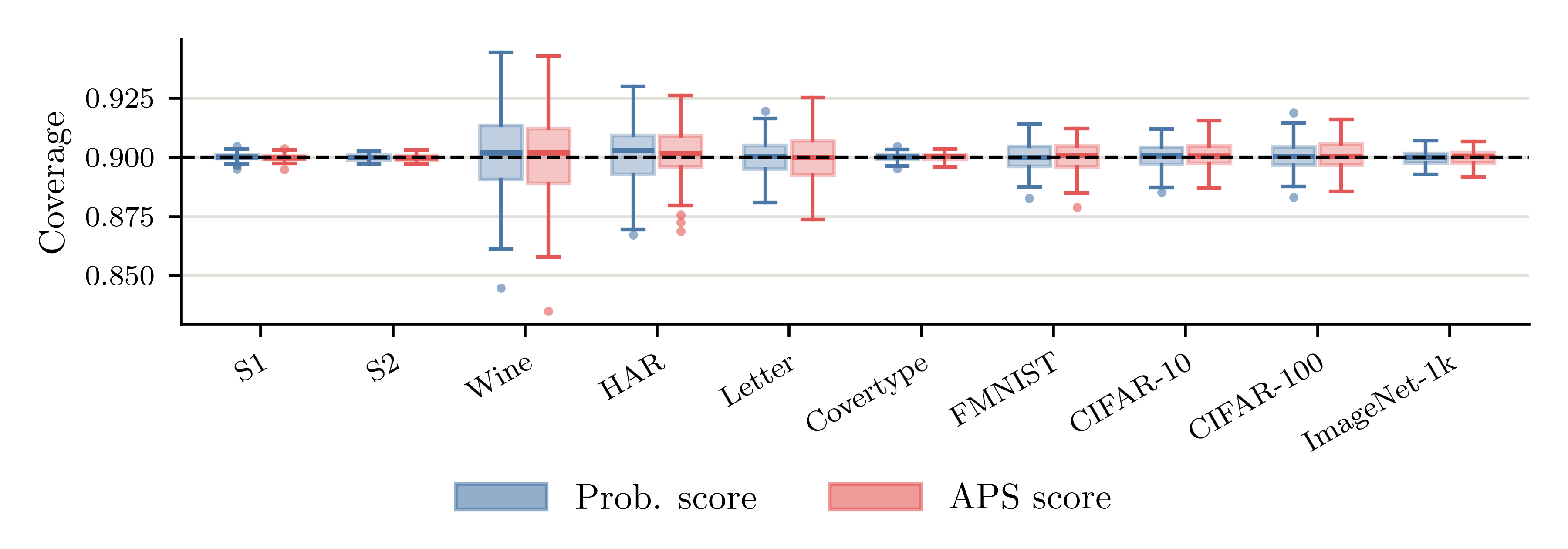
Refer to caption
Figure 5: Empirical marginal coverage of the conformal predictors using (X,Z)(X,Z) over 100 random equal calibration and test splits of the evaluation pool. The dashed line indicates the nominal coverage level 1−α=0.91-\alpha=0.9.

C.5 Accuracy and coverage metrics

We report the top-1 classification accuracy of all models on the held-out evaluation pool. We evaluate models using the augmented features (X,Z)(X,Z), the degraded features (X~,Z)\smash{(\tilde{X},Z)} at each noise level, the base features ZZ, as well as the mask-conditioned model with all candidate features observed. The results are summarized in Table 4.

As expected, classification accuracy generally decreases as features are degraded or removed. The mask-conditioned models also obtain comparable performance to models trained on the full feature set (X,Z)(X,Z), despite supporting predictions given arbitrary subsets of features. The models using the augmented features do not achieve state-of-the-art performance on these classification tasks, since we use simplified architectures and training procedures. Our primary goal is not to maximize predictive accuracy, but to evaluate our theoretical results under realistic levels of model imperfection.

We additionally evaluate the marginal coverage of the conformal predictors using (X,Z)(X,Z) at the nominal coverage level 1−α=0.91-\alpha=0.9, which is used throughout most of our experimental results. For each dataset, we randomly split the evaluation pool in half into calibration and test sets over 100 replicates. As shown in Figure 5, both the probability and APS scores achieve empirical coverage close to the nominal level on all datasets, with larger variability on the datasets with smaller evaluation pools, such as Wine and HAR.

Appendix D Analysis details

We provide additional details on the estimation of the bounds, the evaluation protocols, and the analysis metrics used in our validation and feature selection experiments.

D.1 Estimation of the bounds

To evaluate the conformal mutual information terms in Theorem 2, we estimate Iλ​(X;Y∣Z)I_{\lambda}(X;Y\mid Z) with the plug-in (or oracle) probability distributions on the test set at the calibrated λ^α(i)\smash{\hat{\lambda}_{\alpha}^{\scriptscriptstyle(i)}}. For Theorem 4, we compute I(1)I^{\scriptscriptstyle(1)} in the same way, since Λ^α(1)\smash{\hat{\Lambda}_{\alpha}^{\scriptscriptstyle(1)}} depends only on ZZ. However, the term I(2)I^{\scriptscriptstyle(2)} in the lower bound cannot be computed using a plug-in estimate. Recall that

I(2)=HΛ^α(2)​(Y∣Z)−HΛ^α(2)​(Y∣X,Z).I^{\scriptscriptstyle(2)}=H_{\hat{\Lambda}_{\alpha}^{\scriptscriptstyle(2)}}(Y\mid Z)-H_{\hat{\Lambda}_{\alpha}^{\scriptscriptstyle(2)}}(Y\mid X,Z). (143)

The second term can be evaluated separately for each test point, but the first term is problematic because Λ^α(2)\smash{\hat{\Lambda}_{\alpha}^{\scriptscriptstyle(2)}} depends on both XX and ZZ. In particular,

HΛ^α(2)​(Y∣Z)=𝔼Z​[∑ymin⁡{1,𝔼⁡[p⁡(y∣X,Z)Λ^α(2)|Z]}].H_{\hat{\Lambda}_{\alpha}^{\scriptscriptstyle(2)}}(Y\mid Z)=\mathbb{E}_{Z}\Bigl[\sum\nolimits_{y}\min\Bigl\{1,\,\mathbb{E}\Bigl[\tfrac{p(y\mid X,Z)}{\hat{\Lambda}_{\alpha}^{\scriptscriptstyle(2)}}\Bigm|Z\Bigr]\Bigr\}\Bigr]. (144)

Since the conditional expectation over X|ZX\mid Z lies inside the minimum, computing it requires multiple draws of XX for each ZZ. In the synthetic settings, p⁡(x∣z)p(x\mid z) is known, so we estimate it by Monte Carlo sampling with M=256M=256 draws of X|ZX\mid Z for each test point. For the real-world datasets, we instead average q⁡(y∣xj,zj)/Λ^α(2)​(xj,zj)\smash{q(y\mid x_{j},z_{j})/\hat{\Lambda}_{\alpha}^{\scriptscriptstyle(2)}(x_{j},z_{j})} over the k=10k=10 nearest other neighbors jj of each test point in the evaluation pool. Neighbors are computed using Euclidean distance on the base features ZZ for tabular data and cosine distance on the learned embedding of ZZ for image data.

In the synthetic settings, we use the oracle conditional distributions, so D(i)=0D^{\scriptscriptstyle(i)}=0 exactly. For the real-world datasets, estimating D(i)D^{\scriptscriptstyle(i)} requires the true conditional distribution, so we set D(i)=0D^{\scriptscriptstyle(i)}=0, which is consistent with the plug-in estimates of I(i)I^{\scriptscriptstyle(i)}. We emphasize that the resulting bounds for the real-world datasets are therefore approximate. These approximations do not undermine our validation, since the synthetic settings evaluate the bounds using the true conditional distributions, while the real-world datasets complement these results under realistic model imperfections.

The terms involving miscoverage rates are estimated by the test-set average of

𝟏[Y∉𝒞α(X(2))]−𝟏[Y∉𝒞α(X(1))]λ^α(i).\frac{\mathbf{1}[Y\notin\mathcal{C}_{\alpha}(X^{\scriptscriptstyle(2)})]-\mathbf{1}[Y\notin\mathcal{C}_{\alpha}(X^{\scriptscriptstyle(1)})]}{\hat{\lambda}_{\alpha}^{\scriptscriptstyle(i)}}. (145)

For the APS bounds, we analogously replace λ^α(i)\smash{\hat{\lambda}_{\alpha}^{\scriptscriptstyle(i)}} with Λ^α(i)\smash{\hat{\Lambda}_{\alpha}^{\scriptscriptstyle(i)}}. Since the random threshold is a function of the input, this estimator is unbiased for the corresponding calibration terms in the bounds, conditional on the calibration set.

D.2 Evaluation protocols

As described in Section 5, we reserve a dedicated pool of nevaln_{\mathrm{eval}} samples from each synthetic and real-world dataset for calibration and testing. We next describe how this evaluation pool is used in each experiment.

D.2.1 Validation experiments

We first describe the evaluation protocol for the validation experiments. For each experimental replicate, we sample a calibration dataset of size ncaln_{\mathrm{cal}} and a test dataset of size ntestn_{\mathrm{test}} without replacement from the evaluation pool. The calibration and test datasets are disjoint but do not necessarily partition the entire pool. For a given random seed, the sampled datasets are nested across sample sizes, while different seeds yield independent draws.

For each metric, we consider three regimes: (i) jointly varying ncal=ntestn_{\mathrm{cal}}=n_{\mathrm{test}}, (ii) varying ncaln_{\mathrm{cal}} with ntestn_{\mathrm{test}} fixed, and (iii) varying ntestn_{\mathrm{test}} with ncaln_{\mathrm{cal}} fixed. For the normalized margin and violation rate, we use a logarithmically spaced grid of five to seven points ranging from 100100 to min⁡(10,000,neval/2)\min(10{,}000,n_{\mathrm{eval}}/2), inclusive. Because the bound width becomes visually uninformative at larger sample sizes, we instead use a logarithmically spaced grid from 1010 to min⁡(1,000,neval/2)\min(1{,}000,n_{\mathrm{eval}}/2). In regimes (ii) and (iii), the fixed sample size is set to the maximum of this grid.

Calibration follows the standard split conformal prediction procedure using either the probability score or APS score. For APS, we use the same score randomization draw U∼Unif⁡[0,1]U\sim\mathrm{Unif}[0,1] between the procedures using X(1)X^{\scriptscriptstyle(1)} and X(2)X^{\scriptscriptstyle(2)}. Both procedures are calibrated on the same calibration set and evaluated on the same test set. We estimate Δα\Delta_{\alpha} by the difference in average prediction set size on the test set under X(1)X^{\scriptscriptstyle(1)} and X(2)X^{\scriptscriptstyle(2)}.

We additionally vary the nominal coverage level over 1−α∈{0.8,0.85,0.9,0.95,0.99}1-\alpha\in\{0.8,0.85,0.9,0.95,0.99\}. For these experiments, ncaln_{\mathrm{cal}} and ntestn_{\mathrm{test}} are held fixed at the respective maximum sample sizes used for each metric, i.e., min⁡(10,000,neval/2)\min(10{,}000,n_{\mathrm{eval}}/2) for the normalized margin and violation rate and min⁡(1,000,neval/2)\min(1{,}000,n_{\mathrm{eval}}/2) for the bound width.

For the DPI validation experiments, we follow a similar calibration and evaluation procedure by sampling from the same evaluation pool. We fix the test set size at ntest=min⁡(10,000,neval/2)n_{\mathrm{test}}=\min(10{,}000,n_{\mathrm{eval}}/2) and vary ncal∈{10,100,1,000}n_{\mathrm{cal}}\in\{10,100,1{,}000\}, omitting values of ncaln_{\mathrm{cal}} that exceed neval/2n_{\mathrm{eval}}/2. Within each replicate, the procedures using the augmented and degraded features share the same calibration and test sets. We intentionally consider small calibration sample sizes to illustrate how the normalized DPI gap concentrates as ncaln_{\mathrm{cal}} increases and to demonstrate that finite-sample calibration variability can result in a negative gap at sufficiently small ncaln_{\mathrm{cal}}.

D.2.2 Feature selection experiments

We next describe the evaluation protocol for the feature selection experiments. For each of 10 random seeds, we randomly partition the evaluation pool into three disjoint subsets, using 50%50\% of the samples as a selection set, 25%25\% as a calibration set, and the remaining 25%25\% as a test set. The selection set is used to compute the criteria and determine the feature ordering, while the calibration and test sets are used only to evaluate the resulting sequence. In the synthetic settings, the base features ZZ are always observed, whereas no features are known initially for the real-world datasets.

Note that this setting contrasts with the active feature acquisition (AFA) literature, which typically selects features to acquire for each individual instance and trains dedicated acquisition policies to optimize predictive performance under a feature budget (Shim et al., 2018). We use a different evaluation protocol because our goal is not to propose a competitive AFA method. Instead, we use a simple protocol to empirically probe how the criteria from our theory rank features in practice.

Let SS denote the set of candidate features, initialized as S=∅S=\emptyset. At each step, we evaluate a selection criterion for every remaining candidate XjX_{j} using the predicted probabilities given XS∪{j}X_{S\cup\{j\}}, add the highest-scoring candidate to SS, and repeat until all candidates are exhausted. This yields a single global feature ordering for each criterion and seed, which is shared across all test samples. For each prefix of the ordering, we then calibrate the conformal predictor on the calibration set at nominal coverage 1−α=0.91-\alpha=0.9 and evaluate set size, coverage, and accuracy on the test set.

We compare the following selection criteria, each computed using the predicted probabilities of the oracle or mask-conditioned model as a plug-in estimate.

  • •

    Δα\Delta_{\alpha} (Prob.): the reduction in the average set size using probability score with XS∪{j}X_{S\cup\{j\}};

  • •

    Δα\Delta_{\alpha} (APS): the reduction in the average set size using APS score with XS∪{j}X_{S\cup\{j\}};

  • •

    IλI_{\lambda} (Prob.): the conformal mutual information Iλ​(Xj;Y∣XS)I_{\lambda}(X_{j};Y\mid X_{S}) evaluated at the geometric mean λ=(λ^α(1)​λ^α(2))1/2\smash{\lambda=(\hat{\lambda}_{\alpha}^{\scriptscriptstyle(1)}\hat{\lambda}_{\alpha}^{\scriptscriptstyle(2)})^{1/2}} of the calibrated thresholds using XSX_{S} and XS∪{j}X_{S\cup\{j\}};

  • •

    Shannon MI: the plug-in estimate I^​(Xj;Y∣XS)=H^​(Y∣XS)−H^​(Y∣XS∪{j})\hat{I}(X_{j};Y\mid X_{S})=\hat{H}(Y\mid X_{S})-\hat{H}(Y\mid X_{S\cup\{j\}});

  • •

    Accuracy: the empirical top-1 accuracy gain with XS∪{j}X_{S\cup\{j\}};

  • •

    Random: a uniformly random ordering of the candidate features.

Since the conformal-based criteria require separate calibration data, we use 5-fold cross-fitting within the selection set. We calibrate the thresholds on four folds and evaluate the criterion on the held-out fold, then average the resulting values across folds. The Shannon mutual information and accuracy criteria do not require calibration and are computed directly on the full selection set.

We do not include an analogous IΛI_{\Lambda} criterion for the APS score since it requires the same kk-NN approximation of the conditional expectation over Xj|XSX_{j}\mid X_{S} as described above for I(2)I^{\scriptscriptstyle(2)}. Repeating this approximation for every candidate at every step is computationally expensive and introduces additional approximation error, so we omit this criterion.

D.3 Metrics

We next formalize the evaluation metrics in further detail.

D.3.1 Validation experiments

In the validation experiments, we consider four main metrics: normalized margin, violation rate, normalized width, and normalized DPI gap. Except for the violation rate, we normalize all metrics by the number of classes KK in order to compare across datasets. We next define each metric formally.

Let [L,U][L,U] denote the estimated bounds from Theorem 2 for the probability score or Theorem 4 for APS. When computing the normalized margin, violation rate, and normalized width, we discard replicates with invalid bounds (U<LU<L), which occur in roughly 3%3\% of cases, and average over the remaining random splits of the data. This exclusion does not change our conclusions.

The normalized margin quantifies the magnitude by which the empirical Δα\Delta_{\alpha} falls outside the theoretical bounds for a particular realization of the calibration and test data. Although the theoretical bounds hold exactly for the population quantities under the assumptions of our results, finite-sample Monte Carlo estimation and model approximation on the real-world datasets can lead to empirical violations. We define

Normalized​Margin=d⁡(Δα,[L,U])K=max⁡{L−Δα,Δα−U, 0}K,\mathrm{Normalized\ Margin}=\frac{d(\Delta_{\alpha},[L,U])}{K}=\frac{\max\{L-\Delta_{\alpha},\,\Delta_{\alpha}-U,\,0\}}{K}, (146)

where d⁡(x,ℐ)d(x,\mathcal{I}) denotes the distance from xx to the interval ℐ\mathcal{I}, with d⁡(x,ℐ)=0d(x,\mathcal{I})=0 whenever x∈ℐx\in\mathcal{I}.

The violation rate examines how frequently the empirical Δα\Delta_{\alpha} falls outside the theoretical bounds, providing a binary measure of empirical validity that does not account for the magnitude of a violation. We define

Violation​Rate=ℙ⁡(Δα∉[L,U]),\mathrm{Violation\ Rate}=\mathbb{P}\bigl(\Delta_{\alpha}\notin[L,U]\bigr), (147)

where the probability is estimated over random replicates of the calibration and test data. In practice, we expand the lower and upper bounds by a small slack of 10−410^{-4} to account for floating-point error when computing this metric.

The normalized width measures the informativeness of the bounds through the size of the interval [L,U][L,U]. We define

Normalized​Width=U−LK.\mathrm{Normalized\ Width}=\frac{U-L}{K}. (148)

Since we exclude replicates with U<LU<L, the normalized width is non-negative for every replicate.

Finally, the normalized DPI gap compares the conformal set-size reduction obtained by augmenting the base features ZZ with either XX or its degraded counterpart X~\smash{\tilde{X}}. For each replicate, we use identical test sets to estimate the expected set-size reductions Δα\Delta_{\alpha} and Δ~α\smash{\tilde{\Delta}_{\alpha}} and define

Normalized​DPI​Gap=Δα−Δ~αK.\mathrm{Normalized\ DPI\ Gap}=\frac{\Delta_{\alpha}-\smash{\tilde{\Delta}_{\alpha}}}{K}. (149)

We examine the distribution of this gap across random draws of the calibration and test data.

D.3.2 Feature selection experiments

In the feature selection experiments, we evaluate each criterion by the quality of the conformal predictors obtained along its selection trajectory. Let SjS_{j} denote the first jj candidates acquired under a given criterion. For each jj, we compute the average prediction set size and empirical coverage on the test set using XSjX_{S_{j}} for both the probability score and the APS score. We additionally report the top-1 and top-5 classification accuracy of the model given XSjX_{S_{j}} on the test set.

Let ℰj\mathcal{E}_{j} denote any one of these metrics evaluated using the first jj features. To summarize performance across the entire selection trajectory, we report the average

ℰ¯=1m−1​∑j=1m−1ℰj,\bar{\mathcal{E}}=\frac{1}{m-1}\sum_{j=1}^{m-1}\mathcal{E}_{j}, (150)

where we exclude the cases j=0j=0 and j=mj=m since all criteria observe identical features at the endpoints. Intuitively, ℰ¯\bar{\mathcal{E}} approximates the area under the curve of each metric normalized by mm. This summarizes the performance across all steps rather than at a single fixed budget.

D.4 Implementation details

The validation experiments require evaluating a large number of calibration and test draws across sample sizes, random seeds, nominal coverage levels, feature sets, and conformity scores. To reduce the computational cost, we presort the predicted class probabilities for the evaluation pool and use binary search to efficiently compute the quantities required for each replicate. This optimization is an exact reformulation of the standard computation and does not affect any reported results.

For an evaluation pool of NN samples and KK classes, presorting requires O⁡(N​K​log⁡K)O(NK\log K) time. Each subsequent replicate requires O⁡(ncal​log⁡ncal+ntest​log⁡K)O(n_{\mathrm{cal}}\log n_{\mathrm{cal}}+n_{\mathrm{test}}\log K) time. This provides a substantial computational speedup over directly recomputing the conformal prediction sets, particularly for datasets with large KK such as ImageNet-1k.

The presorting approach does not apply to the feature selection experiments, since the evaluated subsets depend on the selection criterion and the number of possible subsets grows exponentially. Instead, we naively compute the predicted probabilities for each candidate subset at each step.

Appendix E Additional experiments

In this section, we further investigate the empirical behavior of our sandwich bounds for set-size reduction using the probability and APS scores. We then provide additional results for the DPI under different noise levels and report feature selection results across the remaining datasets. Details of the evaluation procedures and metrics are described in Appendix D.

E.1 Sandwich validation results

We provide additional results demonstrating the empirical behavior of Theorems 2 and 4. We first investigate the violation rate of the bounds as we jointly vary ncaln_{\mathrm{cal}} and ntestn_{\mathrm{test}}. We show these results in Figure 6, together with the normalized margin and width results from Figure 3 for comparison.

Consistent with the normalized margin, the violation rate is nonzero at smaller calibration and test set sizes but decreases toward zero as the sample size increases. The main outlier is the Wine dataset using the probability score, for which the violation rate remains high over the evaluated range. This behavior largely reflects the binary nature of the violation rate. The corresponding normalized margin behaves similarly to those of the other datasets, indicating that the violations themselves are small in magnitude.

Comparing the probability and APS scores, we find that the violation rate is typically lower for APS across datasets and sample sizes. The lower violation rate for APS is consistent with its wider bounds, which are easier to satisfy and less sensitive to finite-sample estimation error.

We next examine the normalized margin, violation rate, and normalized width as we independently and jointly vary ncaln_{\mathrm{cal}} and ntestn_{\mathrm{test}} in Figures 7–9. Additionally, we investigate the three metrics across different nominal coverage levels in Figure 10.

Normalized margin (Figure 7).  The magnitude of the empirical violations is driven primarily by the size of the test set. As ntestn_{\mathrm{test}} increases with ncaln_{\mathrm{cal}} fixed, the normalized margin decreases toward zero. In contrast, with ntestn_{\mathrm{test}} fixed, the margin is largely insensitive to ncaln_{\mathrm{cal}}. This suggests that the observed violations primarily arise from finite test-set estimation error.

Refer to caption
Figure 6: We show the normalized margin and violation rate as we jointly vary ncaln_{\mathrm{cal}} and ntestn_{\mathrm{test}} (left and middle) and the normalized width as we vary ncaln_{\mathrm{cal}} while keeping ntestn_{\mathrm{test}} fixed (right). All panels report the mean ±\pm standard error based on 100100 random draws of the calibration and test sets from the fixed evaluation pool.
Refer to caption
Figure 7: We show the normalized margin as we vary ncaln_{\mathrm{cal}} and ntestn_{\mathrm{test}} jointly (left) or independently (middle and right). All panels report the mean ±\pm standard error based on 100100 random draws of the calibration and test sets from the fixed evaluation pool.
Refer to caption
Figure 8: We show the violation rate as we vary ncaln_{\mathrm{cal}} and ntestn_{\mathrm{test}} jointly (left) or independently (middle and right). All panels report the mean ±\pm standard error based on 100100 random draws of the calibration and test sets from the fixed evaluation pool.

Violation rate (Figure 8).  The violation rate exhibits a similar dependence on ntestn_{\mathrm{test}}. When ntestn_{\mathrm{test}} is fixed, the violation rate for APS is low and largely insensitive to ncaln_{\mathrm{cal}}, whereas for the probability score it decreases toward zero as ncaln_{\mathrm{cal}} increases. The Wine dataset is the sole exception, where the violation rate remains between roughly 60%60\% and 80%80\%.

Normalized width (Figure 9).  The normalized width mostly depends on the size of the calibration set and decreases quickly with ncaln_{\mathrm{cal}}. This behavior agrees with our theoretical analysis of the finite-sample calibration terms. As the calibration size increases, the training-conditional miscoverage rates concentrate around the nominal coverage level, causing the finite-sample calibration terms to shrink and the bounds to tighten.

Refer to caption
Figure 9: We show the normalized width as we vary ncaln_{\mathrm{cal}} and ntestn_{\mathrm{test}} jointly (left) or independently (middle and right). All panels report the mean ±\pm standard error based on 100100 random draws of the calibration and test sets from the fixed evaluation pool.
Refer to caption
Figure 10: We show the normalized margin, violation rate, and normalized width as we vary the nominal coverage level 1−α∈{0.8,0.85,0.9,0.95,0.99}1-\alpha\in\{0.8,0.85,0.9,0.95,0.99\}, with ncaln_{\mathrm{cal}} and ntestn_{\mathrm{test}} fixed at their largest values for each dataset. All panels report the mean ±\pm standard error based on 100100 random draws of the calibration and test sets from the fixed evaluation pool.

Nominal coverage levels (Figure 10).  The bounds remain well-behaved across nominal coverage levels 1−α≤0.951-\alpha\leq 0.95 for most datasets (with exceptions for Wine, FMNIST, and CIFAR-10). However, at 1−α=0.991-\alpha=0.99, all three metrics increase sharply for most datasets. We attribute this behavior to sensitivity to the calibrated thresholds λ^α(i)\smash{\hat{\lambda}^{\scriptscriptstyle(i)}_{\alpha}} and Λ^α(i)\smash{\hat{\Lambda}^{\scriptscriptstyle(i)}_{\alpha}}. As the nominal coverage level increases, these thresholds become smaller, which amplifies the finite-sample calibration terms and consequently increases the width of the bounds. The smaller thresholds also increase the variance of the corresponding empirical estimates, leading to larger normalized margins and violation rates at fixed calibration and test sample sizes.

E.2 DPI validation results

We show the distribution of the normalized DPI gap across calibration sample sizes and degradation levels in Figure 11. The results for the medium degradation level (γ=0.5\gamma=0.5) correspond to those reported in Section 5.

Across all degradation levels, the realized gap can be negative for particular draws of the calibration and test data. As the calibration sample size increases, however, the variability of the gap decreases and its distribution generally concentrates around a non-negative mean. Increasing the degradation level also generally increases the average gap as expected, since stronger noise removes more of the information present in XX. These trends hold for both probability score and APS score.

These results further support the interpretation of conformal set-size reduction as a measure of information gain. Theorems 3 and 5 establish an approximate data processing inequality, with finite-sample calibration and model-error terms that allow the DPI gap to be negative. Empirically, the gap is generally non-negative on average, providing evidence of this data processing behavior in practice. At the same time, the negative gaps observed for individual replicates demonstrate that the deviations permitted by our theoretical results do indeed occur in practice.

Refer to caption
Figure 11: We show the normalized DPI gap across calibration sample sizes and degradation levels, using boxplots to summarize 100 random draws of the calibration and test sets. Each column corresponds to a degradation level, and the marker for each dataset is indicated above the corresponding boxplots. For visual clarity, we magnify the yy-axis by 2×2\times and 4×4\times for ncal=100n_{\mathrm{cal}}=100 and ncal=1,000n_{\mathrm{cal}}=1{,}000, respectively. Datasets whose evaluation pool is too small for a given calibration size are omitted.

E.3 Feature selection results

We report feature selection results for all datasets in Table 5, excluding synthetic setting S1 since it has too few candidate features to meaningfully distinguish the criteria.

Across most settings, selection based on set-size reduction yields the smallest prediction sets while typically achieving the best top-5 accuracy. The main exceptions occur for the APS score on Wine and FMNIST. The two Δα\Delta_{\alpha} criteria perform similarly to each other but do not always yield the smallest sets under their own score. Since these differences are often within one standard error, they likely reflect estimation noise in the selection set.

We also evaluate selection using IλI_{\lambda}, which performs similarly to Δα\Delta_{\alpha} under the probability score in the synthetic settings but often yields larger sets on the real-world datasets. We attribute this gap to model imperfection. Theorem 2 brackets Δα\Delta_{\alpha} by conformal mutual information only up to the model error terms D(i)D^{\scriptscriptstyle(i)}, so the plug-in IλI_{\lambda} at the geometric mean of the calibrated thresholds becomes a less precise proxy for Δα\Delta_{\alpha} when these terms are nonzero.

Table 5: We evaluate feature selection performance using conformal set-size reduction. Each row represents one selection criterion and values are reported as mean ±\pm standard error over 10 random splits of the evaluation pool. Arrows indicate the direction of improvement, and the best-performing method for each metric is bolded. Empirical coverage is reported for reference without bolding to indicate that differences in set size are not due to undercoverage.
Dataset Criterion Prob. APS Acc.
𝔼⁡[|𝒞|]\mathbb{E}[|\mathcal{C}|] (↓\downarrow) Cov. 𝔼⁡[|𝒞|]\mathbb{E}[|\mathcal{C}|] (↓\downarrow) Cov. Top-1 (↑\uparrow) Top-5 (↑\uparrow)
S2 Δα\Delta_{\alpha} (Prob.) 11.464±0.03211.464\pm 0.032 0.900±0.0010.900\pm 0.001 11.952±0.02911.952\pm 0.029 0.900±0.0010.900\pm 0.001 0.366±0.0010.366\pm 0.001 0.722±0.000\mathbf{0.722\pm 0.000}
Δα\Delta_{\alpha} (APS) 11.459±0.03311.459\pm 0.033 0.900±0.0010.900\pm 0.001 11.950±0.02911.950\pm 0.029 0.900±0.0010.900\pm 0.001 0.366±0.0010.366\pm 0.001 0.722±0.001\mathbf{0.722\pm 0.001}
IλI_{\lambda} (Prob.) 11.456±0.032\mathbf{11.456\pm 0.032} 0.900±0.0010.900\pm 0.001 11.948±0.028\mathbf{11.948\pm 0.028} 0.900±0.0010.900\pm 0.001 0.366±0.0010.366\pm 0.001 0.722±0.001\mathbf{0.722\pm 0.001}
Shannon MI 11.473±0.03111.473\pm 0.031 0.900±0.0010.900\pm 0.001 11.959±0.02711.959\pm 0.027 0.900±0.0010.900\pm 0.001 0.367±0.001\mathbf{0.367\pm 0.001} 0.722±0.001\mathbf{0.722\pm 0.001}
Accuracy 11.503±0.02911.503\pm 0.029 0.900±0.0010.900\pm 0.001 11.986±0.02611.986\pm 0.026 0.900±0.0010.900\pm 0.001 0.367±0.001\mathbf{0.367\pm 0.001} 0.722±0.001\mathbf{0.722\pm 0.001}
Random 12.207±0.08512.207\pm 0.085 0.900±0.0010.900\pm 0.001 12.670±0.08512.670\pm 0.085 0.900±0.0010.900\pm 0.001 0.354±0.0020.354\pm 0.002 0.707±0.0020.707\pm 0.002
S3 Δα\Delta_{\alpha} (Prob.) 2.239±0.0022.239\pm 0.002 0.900±0.0000.900\pm 0.000 2.629±0.0022.629\pm 0.002 0.900±0.0000.900\pm 0.000 0.750±0.0010.750\pm 0.001 0.952±0.0000.952\pm 0.000
Δα\Delta_{\alpha} (APS) 2.243±0.0022.243\pm 0.002 0.900±0.0000.900\pm 0.000 2.611±0.002\mathbf{2.611\pm 0.002} 0.900±0.0000.900\pm 0.000 0.752±0.0000.752\pm 0.000 0.952±0.0000.952\pm 0.000
IλI_{\lambda} (Prob.) 2.237±0.003\mathbf{2.237\pm 0.003} 0.900±0.0000.900\pm 0.000 2.626±0.0022.626\pm 0.002 0.900±0.0000.900\pm 0.000 0.753±0.0000.753\pm 0.000 0.953±0.000\mathbf{0.953\pm 0.000}
Shannon MI 2.447±0.0052.447\pm 0.005 0.900±0.0000.900\pm 0.000 2.876±0.0062.876\pm 0.006 0.900±0.0000.900\pm 0.000 0.767±0.0000.767\pm 0.000 0.952±0.0000.952\pm 0.000
Accuracy 3.613±0.0203.613\pm 0.020 0.900±0.0000.900\pm 0.000 4.487±0.0294.487\pm 0.029 0.900±0.0000.900\pm 0.000 0.768±0.001\mathbf{0.768\pm 0.001} 0.914±0.0010.914\pm 0.001
Random 3.046±0.1003.046\pm 0.100 0.900±0.0000.900\pm 0.000 3.591±0.1163.591\pm 0.116 0.900±0.0000.900\pm 0.000 0.672±0.0090.672\pm 0.009 0.931±0.0040.931\pm 0.004
Wine Δα\Delta_{\alpha} (Prob.) 2.265±0.034\mathbf{2.265\pm 0.034} 0.904±0.0080.904\pm 0.008 2.387±0.0292.387\pm 0.029 0.905±0.0060.905\pm 0.006 0.553±0.006\mathbf{0.553\pm 0.006} 0.996±0.001\mathbf{0.996\pm 0.001}
Δα\Delta_{\alpha} (APS) 2.279±0.0422.279\pm 0.042 0.902±0.0080.902\pm 0.008 2.378±0.0362.378\pm 0.036 0.904±0.0070.904\pm 0.007 0.548±0.0050.548\pm 0.005 0.995±0.0010.995\pm 0.001
IλI_{\lambda} (Prob.) 2.334±0.0502.334\pm 0.050 0.903±0.0100.903\pm 0.010 2.417±0.0402.417\pm 0.040 0.904±0.0090.904\pm 0.009 0.529±0.0050.529\pm 0.005 0.995±0.0010.995\pm 0.001
Shannon MI 2.288±0.0422.288\pm 0.042 0.900±0.0090.900\pm 0.009 2.383±0.0362.383\pm 0.036 0.903±0.0080.903\pm 0.008 0.550±0.0050.550\pm 0.005 0.995±0.0010.995\pm 0.001
Accuracy 2.284±0.0422.284\pm 0.042 0.904±0.0090.904\pm 0.009 2.371±0.032\mathbf{2.371\pm 0.032} 0.904±0.0070.904\pm 0.007 0.552±0.0040.552\pm 0.004 0.996±0.001\mathbf{0.996\pm 0.001}
Random 2.420±0.0462.420\pm 0.046 0.906±0.0070.906\pm 0.007 2.506±0.0462.506\pm 0.046 0.902±0.0070.902\pm 0.007 0.507±0.0050.507\pm 0.005 0.995±0.0010.995\pm 0.001
HAR Δα\Delta_{\alpha} (Prob.) 0.912±0.0050.912\pm 0.005 0.899±0.0050.899\pm 0.005 0.963±0.0020.963\pm 0.002 0.900±0.0020.900\pm 0.002 0.971±0.001\mathbf{0.971\pm 0.001} 1.000±0.000\mathbf{1.000\pm 0.000}
Δα\Delta_{\alpha} (APS) 0.909±0.006\mathbf{0.909\pm 0.006} 0.896±0.0060.896\pm 0.006 0.960±0.002\mathbf{0.960\pm 0.002} 0.899±0.0010.899\pm 0.001 0.970±0.0010.970\pm 0.001 1.000±0.000\mathbf{1.000\pm 0.000}
IλI_{\lambda} (Prob.) 0.918±0.0050.918\pm 0.005 0.897±0.0050.897\pm 0.005 0.961±0.0010.961\pm 0.001 0.898±0.0020.898\pm 0.002 0.968±0.0020.968\pm 0.002 1.000±0.000\mathbf{1.000\pm 0.000}
Shannon MI 0.916±0.0050.916\pm 0.005 0.898±0.0050.898\pm 0.005 0.960±0.001\mathbf{0.960\pm 0.001} 0.899±0.0020.899\pm 0.002 0.968±0.0020.968\pm 0.002 1.000±0.000\mathbf{1.000\pm 0.000}
Accuracy 0.910±0.0050.910\pm 0.005 0.898±0.0040.898\pm 0.004 0.961±0.0030.961\pm 0.003 0.900±0.0010.900\pm 0.001 0.971±0.001\mathbf{0.971\pm 0.001} 1.000±0.000\mathbf{1.000\pm 0.000}
Random 0.999±0.0150.999\pm 0.015 0.900±0.0040.900\pm 0.004 1.064±0.0171.064\pm 0.017 0.899±0.0020.899\pm 0.002 0.934±0.0050.934\pm 0.005 1.000±0.000\mathbf{1.000\pm 0.000}
Letter Δα\Delta_{\alpha} (Prob.) 2.753±0.016\mathbf{2.753\pm 0.016} 0.898±0.0030.898\pm 0.003 3.358±0.019\mathbf{3.358\pm 0.019} 0.900±0.0010.900\pm 0.001 0.756±0.0010.756\pm 0.001 0.926±0.000\mathbf{0.926\pm 0.000}
Δα\Delta_{\alpha} (APS) 2.835±0.0382.835\pm 0.038 0.898±0.0020.898\pm 0.002 3.398±0.0323.398\pm 0.032 0.900±0.0010.900\pm 0.001 0.758±0.0020.758\pm 0.002 0.924±0.0010.924\pm 0.001
IλI_{\lambda} (Prob.) 2.824±0.0222.824\pm 0.022 0.898±0.0030.898\pm 0.003 3.385±0.0283.385\pm 0.028 0.901±0.0020.901\pm 0.002 0.760±0.0010.760\pm 0.001 0.924±0.0010.924\pm 0.001
Shannon MI 2.801±0.0192.801\pm 0.019 0.899±0.0030.899\pm 0.003 3.399±0.0263.399\pm 0.026 0.901±0.0010.901\pm 0.001 0.758±0.0010.758\pm 0.001 0.924±0.0010.924\pm 0.001
Accuracy 2.879±0.0202.879\pm 0.020 0.899±0.0020.899\pm 0.002 3.415±0.0223.415\pm 0.022 0.901±0.0010.901\pm 0.001 0.763±0.001\mathbf{0.763\pm 0.001} 0.922±0.0010.922\pm 0.001
Random 4.459±0.1844.459\pm 0.184 0.897±0.0020.897\pm 0.002 5.054±0.1745.054\pm 0.174 0.900±0.0010.900\pm 0.001 0.642±0.0110.642\pm 0.011 0.871±0.0070.871\pm 0.007
Covertype Δα\Delta_{\alpha} (Prob.) 1.010±0.001\mathbf{1.010\pm 0.001} 0.900±0.0010.900\pm 0.001 1.139±0.0011.139\pm 0.001 0.900±0.0000.900\pm 0.000 0.906±0.001\mathbf{0.906\pm 0.001} 1.000±0.000\mathbf{1.000\pm 0.000}
Δα\Delta_{\alpha} (APS) 1.011±0.0011.011\pm 0.001 0.900±0.0010.900\pm 0.001 1.140±0.0011.140\pm 0.001 0.900±0.0000.900\pm 0.000 0.906±0.000\mathbf{0.906\pm 0.000} 1.000±0.000\mathbf{1.000\pm 0.000}
IλI_{\lambda} (Prob.) 1.010±0.001\mathbf{1.010\pm 0.001} 0.900±0.0010.900\pm 0.001 1.138±0.001\mathbf{1.138\pm 0.001} 0.900±0.0000.900\pm 0.000 0.906±0.001\mathbf{0.906\pm 0.001} 1.000±0.000\mathbf{1.000\pm 0.000}
Shannon MI 1.010±0.001\mathbf{1.010\pm 0.001} 0.900±0.0010.900\pm 0.001 1.138±0.001\mathbf{1.138\pm 0.001} 0.900±0.0000.900\pm 0.000 0.906±0.001\mathbf{0.906\pm 0.001} 1.000±0.000\mathbf{1.000\pm 0.000}
Accuracy 1.010±0.001\mathbf{1.010\pm 0.001} 0.900±0.0010.900\pm 0.001 1.139±0.0011.139\pm 0.001 0.900±0.0000.900\pm 0.000 0.906±0.001\mathbf{0.906\pm 0.001} 1.000±0.000\mathbf{1.000\pm 0.000}
Random 1.593±0.0351.593\pm 0.035 0.901±0.0010.901\pm 0.001 1.731±0.0361.731\pm 0.036 0.900±0.0000.900\pm 0.000 0.717±0.0110.717\pm 0.011 0.996±0.0000.996\pm 0.000
FMNIST Δα\Delta_{\alpha} (Prob.) 1.020±0.002\mathbf{1.020\pm 0.002} 0.900±0.0020.900\pm 0.002 1.220±0.0041.220\pm 0.004 0.898±0.0010.898\pm 0.001 0.903±0.0010.903\pm 0.001 0.998±0.000\mathbf{0.998\pm 0.000}
Δα\Delta_{\alpha} (APS) 1.028±0.0021.028\pm 0.002 0.901±0.0020.901\pm 0.002 1.167±0.0021.167\pm 0.002 0.899±0.0010.899\pm 0.001 0.901±0.0010.901\pm 0.001 0.998±0.000\mathbf{0.998\pm 0.000}
IλI_{\lambda} (Prob.) 1.040±0.0021.040\pm 0.002 0.901±0.0020.901\pm 0.002 1.166±0.0021.166\pm 0.002 0.899±0.0010.899\pm 0.001 0.899±0.0010.899\pm 0.001 0.998±0.000\mathbf{0.998\pm 0.000}
Shannon MI 1.037±0.0021.037\pm 0.002 0.901±0.0020.901\pm 0.002 1.163±0.002\mathbf{1.163\pm 0.002} 0.899±0.0010.899\pm 0.001 0.901±0.0010.901\pm 0.001 0.998±0.000\mathbf{0.998\pm 0.000}
Accuracy 1.023±0.0021.023\pm 0.002 0.902±0.0020.902\pm 0.002 1.220±0.0031.220\pm 0.003 0.898±0.0010.898\pm 0.001 0.904±0.001\mathbf{0.904\pm 0.001} 0.997±0.0000.997\pm 0.000
Random 1.064±0.0041.064\pm 0.004 0.902±0.0020.902\pm 0.002 1.259±0.0041.259\pm 0.004 0.899±0.0010.899\pm 0.001 0.896±0.0010.896\pm 0.001 0.997±0.0000.997\pm 0.000
CIFAR-10 Δα\Delta_{\alpha} (Prob.) 1.489±0.007\mathbf{1.489\pm 0.007} 0.899±0.0030.899\pm 0.003 1.774±0.0071.774\pm 0.007 0.899±0.0010.899\pm 0.001 0.795±0.0020.795\pm 0.002 0.986±0.000\mathbf{0.986\pm 0.000}
Δα\Delta_{\alpha} (APS) 1.507±0.0061.507\pm 0.006 0.900±0.0020.900\pm 0.002 1.742±0.004\mathbf{1.742\pm 0.004} 0.900±0.0010.900\pm 0.001 0.793±0.0020.793\pm 0.002 0.986±0.000\mathbf{0.986\pm 0.000}
IλI_{\lambda} (Prob.) 1.592±0.0101.592\pm 0.010 0.900±0.0020.900\pm 0.002 1.774±0.0081.774\pm 0.008 0.899±0.0010.899\pm 0.001 0.781±0.0010.781\pm 0.001 0.984±0.0000.984\pm 0.000
Shannon MI 1.561±0.0071.561\pm 0.007 0.899±0.0020.899\pm 0.002 1.756±0.0051.756\pm 0.005 0.899±0.0010.899\pm 0.001 0.785±0.0010.785\pm 0.001 0.984±0.0000.984\pm 0.000
Accuracy 1.502±0.0081.502\pm 0.008 0.901±0.0020.901\pm 0.002 1.780±0.0041.780\pm 0.004 0.900±0.0010.900\pm 0.001 0.800±0.002\mathbf{0.800\pm 0.002} 0.985±0.0000.985\pm 0.000
Random 1.711±0.0121.711\pm 0.012 0.900±0.0020.900\pm 0.002 1.996±0.0151.996\pm 0.015 0.900±0.0020.900\pm 0.002 0.772±0.0030.772\pm 0.003 0.978±0.0010.978\pm 0.001
CIFAR-100 Δα\Delta_{\alpha} (Prob.) 12.683±0.10012.683\pm 0.100 0.904±0.0020.904\pm 0.002 15.661±0.12715.661\pm 0.127 0.902±0.0020.902\pm 0.002 0.466±0.0020.466\pm 0.002 0.753±0.002\mathbf{0.753\pm 0.002}
Δα\Delta_{\alpha} (APS) 12.594±0.088\mathbf{12.594\pm 0.088} 0.902±0.0020.902\pm 0.002 15.472±0.129\mathbf{15.472\pm 0.129} 0.902±0.0020.902\pm 0.002 0.467±0.002\mathbf{0.467\pm 0.002} 0.753±0.002\mathbf{0.753\pm 0.002}
IλI_{\lambda} (Prob.) 13.700±0.11513.700\pm 0.115 0.901±0.0020.901\pm 0.002 16.438±0.11016.438\pm 0.110 0.901±0.0020.901\pm 0.002 0.456±0.0030.456\pm 0.003 0.740±0.0020.740\pm 0.002
Shannon MI 13.763±0.11513.763\pm 0.115 0.902±0.0020.902\pm 0.002 16.597±0.14516.597\pm 0.145 0.902±0.0020.902\pm 0.002 0.458±0.0030.458\pm 0.003 0.741±0.0020.741\pm 0.002
Accuracy 12.872±0.13012.872\pm 0.130 0.902±0.0020.902\pm 0.002 15.877±0.15815.877\pm 0.158 0.901±0.0020.901\pm 0.002 0.467±0.003\mathbf{0.467\pm 0.003} 0.752±0.0020.752\pm 0.002
Random 14.243±0.25314.243\pm 0.253 0.902±0.0030.902\pm 0.003 17.189±0.22417.189\pm 0.224 0.902±0.0030.902\pm 0.003 0.454±0.0020.454\pm 0.002 0.737±0.0020.737\pm 0.002
ImageNet-1k Δα\Delta_{\alpha} (Prob.) 47.159±0.297\mathbf{47.159\pm 0.297} 0.901±0.0010.901\pm 0.001 58.993±0.35258.993\pm 0.352 0.900±0.0010.900\pm 0.001 0.476±0.0010.476\pm 0.001 0.711±0.0010.711\pm 0.001
Δα\Delta_{\alpha} (APS) 47.262±0.32247.262\pm 0.322 0.901±0.0010.901\pm 0.001 58.155±0.337\mathbf{58.155\pm 0.337} 0.901±0.0010.901\pm 0.001 0.475±0.0010.475\pm 0.001 0.711±0.0010.711\pm 0.001
IλI_{\lambda} (Prob.) 51.958±0.44351.958\pm 0.443 0.901±0.0010.901\pm 0.001 63.887±0.35963.887\pm 0.359 0.900±0.0010.900\pm 0.001 0.472±0.0010.472\pm 0.001 0.707±0.0010.707\pm 0.001
Shannon MI 55.959±0.35855.959\pm 0.358 0.900±0.0010.900\pm 0.001 68.675±0.32068.675\pm 0.320 0.900±0.0010.900\pm 0.001 0.471±0.0010.471\pm 0.001 0.705±0.0010.705\pm 0.001
Accuracy 51.504±0.49451.504\pm 0.494 0.900±0.0010.900\pm 0.001 64.796±0.58164.796\pm 0.581 0.900±0.0010.900\pm 0.001 0.480±0.001\mathbf{0.480\pm 0.001} 0.713±0.001\mathbf{0.713\pm 0.001}
Random 58.187±0.52258.187\pm 0.522 0.901±0.0010.901\pm 0.001 72.623±0.61672.623\pm 0.616 0.900±0.0010.900\pm 0.001 0.472±0.0010.472\pm 0.001 0.704±0.0010.704\pm 0.001
Refer to caption
Figure 12: We show the expected set size using the probability score and APS score against the fraction of candidate features selected. Each curve is the mean over 10 random splits of the evaluation pool. We show only the first half of the selection trajectory, after which the curves largely coincide. On S3 and CIFAR-100, the gap between Δα\Delta_{\alpha} and Shannon MI is concentrated in the early steps, which becomes diluted when averaging over the full trajectory.

The metrics in Table 5 are averaged over all intermediate steps of the feature ordering. Since every criterion eventually selects all candidate features, the set sizes converge as more features are acquired, and averaging over the full trajectory can mask differences that occur early in selection. To examine this, we show the expected set size at each step for the three datasets from Table 1 in Figure 12. The Δα\Delta_{\alpha} criteria yield noticeably smaller sets than Shannon MI when only a small fraction of the candidates has been selected for S3 and CIFAR-100. On Letter, Δα\Delta_{\alpha} using the probability score provides only a small improvement throughout the trajectory.

E.4 Subset-specific model ablation

In the feature selection experiments, the selection criteria and the evaluation both rely on a single mask-conditioned model. A difference between two criteria could therefore reflect how well this model fits particular subsets of features, rather than the information those features carry about YY. To test for this effect, we retrain a subset-specific model for each selected subset on CIFAR-100.

For each criterion and random split, we take the feature ordering from the main experiment and consider its first k∈{1,2,4,8}k\in\{1,2,4,8\} candidates, since the difference between the criteria is concentrated in the early steps of selection (Figure 12). We train a separate classification head on each resulting subset of the frozen backbone representation, using the same architecture and hyperparameters as the mask-conditioned head but without masking. Each subset-specific head is then calibrated and evaluated on the same data as the mask-conditioned model.

Table 6 reports the difference in expected set size between Shannon MI and Δα\Delta_{\alpha} under both models. For simplicity, each Δα\Delta_{\alpha} criterion is evaluated under its own score. The subset-specific models yield smaller sets than the mask-conditioned model for every criterion, and the advantage of Δα\Delta_{\alpha} decreases when averaged over kk from 4.074.07 to 1.891.89 under the probability score and from 3.843.84 to 2.112.11 under the APS score. However, Δα\Delta_{\alpha} continues to yield smaller sets at every kk, with the largest differences in the first two steps.

Table 6: Difference in expected set size between Shannon MI and Δα\Delta_{\alpha} on CIFAR-100 when each feature ordering is evaluated with the mask-conditioned model or with subset-specific models. Positive values indicate that Δα\Delta_{\alpha} yields smaller sets. Values are reported as mean ±\pm standard error over 10 random splits of the evaluation pool.
Prob. APS
kk Mask-cond. Subset-specific Mask-cond. Subset-specific
1 3.75±0.363.75\pm 0.36 2.49±0.322.49\pm 0.32 3.59±0.403.59\pm 0.40 2.33±0.352.33\pm 0.35
2 5.81±0.465.81\pm 0.46 4.06±0.354.06\pm 0.35 5.24±0.545.24\pm 0.54 3.87±0.463.87\pm 0.46
4 3.71±0.333.71\pm 0.33 0.42±0.240.42\pm 0.24 2.98±0.672.98\pm 0.67 1.32±0.311.32\pm 0.31
8 3.00±0.463.00\pm 0.46 0.58±0.320.58\pm 0.32 3.56±0.643.56\pm 0.64 0.91±0.280.91\pm 0.28
Avg. 4.07±0.274.07\pm 0.27 1.89±0.141.89\pm 0.14 3.84±0.413.84\pm 0.41 2.11±0.142.11\pm 0.14

text

Appendix F Compute resources

All training and analysis were performed on a single machine running Ubuntu 24.04 with 32 GB of RAM and an NVIDIA GeForce RTX 5070 Ti GPU. The hyperparameter grid search required approximately 10 hours and subsequent model training required approximately 12 hours. The validation experiments were run on a single CPU thread without GPU acceleration, whereas the feature selection experiments evaluated the mask-conditioned models on the GPU. All downstream analyses required approximately 4 hours in total.

Appendix G Experimental assets

We obtain the Human Activity Recognition dataset (Reyes-Ortiz et al., 2013) directly from the UCI Machine Learning Repository, available under the CC BY 4.0 license. For ImageNet-1k, we use the 64×6464\times 64 downsampled version of Chrabaszcz et al. (2017), which is made available through the ChocolateDave/imagenet-64 mirror on Hugging Face. The pretrained ResNet-18 weights (He et al., 2016) are the IMAGENET1K_V1 weights distributed with torchvision. All remaining datasets are obtained through OpenML or torchvision, with their original sources cited in Section 5 and Appendix B. Code for reproducing our analyses will be released upon publication.