Moving Forward with Video Saliency: A New Dataset and Benchmark where Motion Matters
Abstract
Video saliency prediction attempts to capture more natural human visual behaviour than static image saliency, and is inherently harder to model due to the additional temporal dimension. Video saliency benchmarks rest on an implicit premise that predicting gaze on video requires utilizing temporal activity distributed across frames. Prior work has challenged this premise, showing that a deliberately static baseline recovers a significant fraction of the explainable gaze information on LEDOV, a popular video saliency dataset, without integrating temporal context, and that video saliency models fail in the same places as this static baseline. We first verify that this diagnosis still stands: under a more capable gold standard than the original analysis used, and an updated panel of recent architectures, the strongest temporal architecture in the panel still does not seem to substantially improve over a fine-tuned static baseline. However, it remains unclear whether the marginal gain reflects limitations of current temporal architectures or a lack of genuinely temporal patterns in the benchmark itself. We introduce SalTempto, a new video saliency benchmark with greater dynamism: 224 one-minute clips of highly dynamic content, sourced from the HACS-Segments action dataset so that each clip contains an event together with its lead-up and aftermath, with gaze recordings from up to 16 subjects and a training split for adapting pretrained models. On SalTempto, the same fine-tuned static baseline recovers only about 13% of the headroom above the centerbias, against more than half on LEDOV. The strongest fine-tuned temporal architecture shows a substantial gain in performance over the static baseline, indicating that it does capture meaningfully more temporal information, which LEDOV fails to measure. Yet, even this SoTA model still leaves nearly half of SalTempto’s headroom unexplained, indicating that there is still a lot of room for improvement in the field of video saliency. In addition, manual examination of SalTempto recordings allows us to describe three human visual tendencies that models tend to miss: object permanence despite occlusion, scene inertia, and anticipatory saccades. SalTempto releases with raw visual recordings and training and evaluation videos. Link to anonymous repository: https://huggingface.co/datasets/bethgelab/video_saliency.
1 Introduction
Video saliency models predict where people tend to look when viewing a video. Their predictions serve as attention priors in content-aware video compression, foveated rendering, and evaluation of visual interfaces, and they are the primary computational account of how human attention responds to events as they unfold. What separates the video problem from image saliency is this temporal component: a video model should use viewing history together with scene dynamics to predict where human attention will flow, not only what draws attention in the current frame being observed. Video saliency models are accordingly built on temporal architectures such as recurrent backbones, 3D convolutions, and transformers. They rely on the implicit premise that predicting visual saliency in video requires reasoning across frames. Tangemann et al. (2020) tested this premise on LEDOV (Jiang et al., 2018), reporting that a static baseline recovers at least 75 % of the net explainable gaze information (based on a gold standard model setting an upper bound estimate on performance) without integrating temporal information. Their probe outperformed the state-of-the-art temporal models of the time on standard saliency map evaluation metrics; visual inspection of its failure cases identified clear temporal effects on gaze that are present in LEDOV but rare and not captured by the evaluated panel of models. The implication is uncomfortable: progress on LEDOV cannot reliably be read as progress on temporal modelling, with evaluations on other video saliency datasets presenting their own problems as discussed in later sections. The benchmark needed to test the temporal capabilities of video saliency models requires a stand-alone dataset with greater dynamism, on which static features cannot already do most of the work.
Here, we verify that Tangemann et al.’s diagnosis still holds despite progress in video saliency models that incorporate temporal aspects. Against a more capable gold standard than the original analysis used (§3), and an updated panel of 13 architectures now including post-2020 video saliency models, the static baseline still recovers 56 % of the headroom above centerbias on LEDOV. The strongest current temporal model reaches 75 %, showing only a 19-point improvement over the static baseline. It remains unclear whether this marginal gap reflects limitations of current temporal architectures or a lack of genuinely temporal patterns in LEDOV itself. We perform additional analysis on LEDOV’s fixation distributions, and find that gaze targets cluster spatially even across time within LEDOV videos. Consequently, one frame’s gold-standard density predicts nearly 30% of the net available gaze information of another arbitrary frame in a video (App. C). In other words, models usually do not face the challenge of tracking salient regions that drift spatially over time.
To overcome these problems, we introduce SalTempto: 224 one-minute clips of highly dynamic content, sourced from HACS-Segments (Zhao et al., 2019) so that each clip contains an annotated event together with its lead-up and aftermath, with gaze recordings from up to 16 free-viewing subjects. The resulting foreground dynamics yield wider within-video gaze dispersion than LEDOV. On SalTempto, gaze targets shift between frames to a degree that models must actually attend to salient content over time to meaningfully predict gaze targets (App. C). A fine-tuned static baseline accordingly recovers a much smaller fraction of the available gaze information than on LEDOV, while the strongest temporal architecture shows a substantial gain over the static baseline. This indicates that current architectures measurably capture temporal structure when given a benchmark that surfaces it. Yet, the same architecture leaves 41.5 % of SalTempto’s headroom unexplained (§4), indicating that the video saliency problem is far from solved. In addition, the length of frames, diversity of content, and dense gaze recordings allow us to identify three additional viewer behaviours on video data that models tend to miss: object permanence despite occlusion, scene inertia, and anticipatory saccades (§4).
2 Related work and existing datasets
Among recent video saliency benchmarks like DHF1K (Wang et al., 2018, 1000 videos, 17 subjects), DIEM (Mital et al., 2011), Hollywood-2 and UCF-Sports (Mathe and Sminchisescu, 2015), the LEDOV dataset (Jiang et al., 2018, 538 videos, 32 subjects) has become a preferred choice for fine-tuning and evaluating new architectures. Each of the other video saliency benchmarks falls short on at least one criterion essential to the diagnostic. DHF1K data is known to have artefacts in the published fixation masks (Tangemann et al., 2020). Additionally, DHF1K’s released gaze maps do not preserve per-subject identification, preventing the leave-one-subject-out gold-standard computation that the diagnostic relies on (§3). Hollywood-2 and UCF-Sports (Mathe and Sminchisescu, 2015) record gaze under task-aware observation rather than free-viewing, as subjects were performing action recognition during data collection. They also confine their stimulus distributions to a single content domain (movie scenes for Hollywood-2; sporting scenarios for UCF-Sports), limiting their reach as general-purpose video saliency benchmarks. DIEM (84 videos) was recorded with audio playback and heterogeneous recording setups; we report a zero-shot comparison on it in App. B for completeness despite the confounders. LEDOV is the original target for prior work, the preferred choice for fine-tuning new video saliency architectures, and a free-viewing video saliency benchmark.
Tangemann et al. (2020) introduced the static-recoverability diagnostic together with DeepGaze MR (DG-MR), a static baseline built for the measurement, and applied both to LEDOV with the result summarised in §1. To direct subsequent development, they assembled a meta-dataset of temporally demanding examples drawn from existing fixations on existing clips; a stand-alone benchmark with greater dynamism, on which a static baseline cannot already do most of the work, was not part of that contribution and is what SalTempto provides.
3 Methods
3.1 SalTempto Dataset Creation
Source dataset and stimulus selection. An important prerequisite for capturing temporal effects is the use of videos that are long enough to contain temporal variations. We obtain this structure from HACS-Segments (Zhao et al., 2019), a video dataset spanning 200 categories whose annotations mark the start and end of recognisable actions within each clip. Actions, including their beginning and ending, inherently involve temporal dynamics, leading to highly dynamic and varied temporal effects being present in the final dataset. Videos from this dataset also contain other dynamic events like camera motion or scene cuts, which are viewed by observers and contribute to gaze dynamics. The broad range of categories further ensures greater variance in the presented stimuli. From the HACS pool we filter by resolution () and sample 224 clips satisfying action-segment positioning constraints: each clip contains an annotated action segment beginning at 15 s, with midpoint 30 s, and ending before clip end. This construction yields measurably greater within-video gaze dispersion than LEDOV (App. C).
Fixation collection. 16 participants (9 female, 7 male; mean age 28.6) with normal or corrected-to-normal vision contributed gaze recordings with informed consent. Each training video received gaze from 3 subjects, while each validation and test video was viewed by all 16 subjects. This reflects different tradeoffs between video diversity and density estimation quality: for training models, we benefit from having diverse videos at the cost of subject diversity per video (which is unproblematic for point objectives like fixation log-likelihood). Additionally, per-subject viewing tendencies do not contribute significant information (Agrawal et al., 2026a) especially under unknown viewer identity, therefore subject biases are negligible. On the validation and test splits, we need enough samples for estimating gold standard densities for reliable analyses and case studies, hence we trade-off video quantity for more gaze samples under constant budget, as is common in such studies (Schwetlick et al., 2024). Subjects viewed stimuli on a VIEWPixx 3D monitor refreshed at 120 Hz, head-stabilised by a 50 cm chin rest, while their gaze was sampled at 500 Hz by an EyeLink 1000 calibrated with a 5-point procedure and drift-checked between blocks (off-screen samples excluded). There was no audio present in the stimuli. When starting the experiment, a 5-point calibration was performed, followed up by a validation. Every participant was instructed to view 50 videos, without giving any task. Each stimulus was starting with a fixation cross in the center. Between two stimuli, the participant had the choice to take a break as long as they want and before continuing a drift check was performed by displaying a fixation cross at the center. If the measured gaze position was off by >2°, the calibration was repeated to ensure accurate gaze positions. The stimuli videos for each subject were separated into 20 validation videos and 30 training videos. It was randomized if the trial starts with a training or validation video. Additionally, the order of the videos was randomized to minimize potential order effects like fatigue, contextual biases and stimulus-specific biases.
Per-frame gaze positions used in the analyses of §4 are obtained by binning the per-subject gaze stream into video frames, preserving subject identity. The leave-one-subject-out gold-standard computation in §3.2 also operates on the per-subject binned positions. SalTempto releases the underlying raw 500 Hz trajectories alongside the binned positions, so downstream consumers can recover the saccade and smooth-pursuit dynamics that frame-averaging or fixation-stabilisation would discard.
Splits and release. SalTempto is split into 204 training videos, 10 validation videos, and 10 test videos. In video-hours this is 3.4 h of training video and 0.17 h each of validation and test video, against 1.52 h and 0.13 h for LEDOV; in observer-hours, 8.6 h of training gaze and 2.7 h each for validation and test. Training and validation videos are released publicly with eye-tracking data for both eyes, and additional data such as pupil sizes and sample timestamps at every recording. The test split videos are publicly available, with held-out recordings providing a reference point that guards against benchmark overfitting and lets the field track whether the static-recoverable gap closes as models evolve. On acceptance, SalTempto will be released as a hosted video saliency benchmark.
3.2 The SalTempto Benchmark
Models and fine-tuning protocol. We benchmark 13 architectures: DeepGaze MR (DG-MR), the static baseline introduced by Tangemann et al. (2020), and twelve temporal models spanning from older architectures to the recent state-of-the-art models: SalFoM (Moradi et al., 2024), TMFI-Net (Zhou et al., 2023), ViNet-{S, A, E} (Jain et al., 2021), TASED-Net (Min and Corso, 2019), TinyHD-{single, multi} (Hu et al., 2023), UniformerSal-{Spatial, SpatioTemporal} (Li et al., 2022), and UNISAL-{Spatial, SpatioTemporal} (Droste et al., 2020). The released checkpoints for DG-MR and UniformerSal were trained on LEDOV by their original authors; the remaining ten models’ released checkpoints were trained primarily on DHF1K.
All models are evaluated zero-shot from their released checkpoints. In addition, we fine-tune both DG-MR (static baseline) and SalFoM on each dataset’s training split and evaluate them as well. We select SalFoM as the temporal architecture for fine-tuning because it is the strongest model in the panel. We did not run additional fine-tuning of DG-MR on LEDOV because the released checkpoint was already trained on LEDOV. Fine-tuning ran for roughly 10 h (DG-MR) and 12 h (SalFoM) on a single NVIDIA A100; all other evaluations are inference only. As a within-architecture control, we also evaluate the fine-tuned SalFoM with its temporal context removed, repeating the target frame across the model’s full context window so that the input carries no motion (App. B).
Centerbias. Humans have a tendency to fixate at the center of a scene. The data collection pipeline further exacerbates this tendency by starting each recording session with a central fixation. This centerbias serves as a fundamental prior in studies of visual attention, as it is easy to model and accounts for both data collection biases and natural viewing behaviour. Furthermore, benchmarking against the centerbias ensures that models are evaluated based on the ability to predict meaningful information, rather than exploiting trivial spatial biases (Kümmerer et al., 2016; Kümmerer and Bethge, 2023; Agrawal et al., 2026b). Each dataset’s centerbias is a Gaussian KDE on training fixations, with bandwidth chosen by grid search on held-out log-likelihood: on SalTempto, on LEDOV. The different optima reflect each dataset’s fixation spread, not a methodological asymmetry.
Gold standard. Following the recently proposed method for estimating inter-observer consistency by Agrawal et al. (2026b), our per-frame gold standard is a 4-component mixture consisting of leave-one-subject-out Abramson KDE, a uniform prior, the dataset’s centerbias, and the fine-tuned SalFoM model predictions. The mixture weights are chosen per frame by the held-out-subject fixation likelihood. The gold standard is an estimator of maximum achievable performance. While the KDE captures spatial consistency across observers within a frame, the SalFoM model is used to account for more semantic and other consistencies (such as temporal aspects) across frames and videos. As noted by Agrawal et al. (2026b), without the deep learning component in the mixture, the upper bound estimate achieves a LL of approximately 2 bits/fix on LEDOV; SalFoM achieves approximately 2.9 bits/fix in zero-shot evaluation, and exceeds 3.0 bits/fix post fine-tuning, showing that accounting for semantic, cross-frame and video consistency is crucial for making the “upper bound” trustworthy.
Evaluation metrics. Following Kümmerer et al. (2015); Kümmerer and Bethge (2023), we base the bulk of our analysis and evaluations on information-theoretic metrics. Specifically, we use the Log-Likelihood (LL) predicted by a model at a ground-truth gaze point as a measure of how well it predicts the region to be salient to humans. This also allows a direct comparison against the centerbias prior: the Information Gain (IG) a model captures over the centerbias can be expressed naturally as . The gap between the centerbias (trivially achievable performance) and the gold standard (upper performance bound) a model captures is summarized via Information Gain Explained (IGE; defined in App. A). The gold standard enters only the denominator of IGE, which is shared by every model on a dataset; LL, IG, and the resulting model rankings do not depend on it. We additionally report standard saliency-evaluation metrics in the same appendix: KL divergence (KLD) against a Gaussian-blurred fixation density map, Pearson correlation (CC), histogram similarity (SIM), area under the ROC curve (AUC), and normalized scanpath saliency (NSS); see Bylinskii et al. (2019) for definitions and a comparative analysis.
4 Dataset Analysis and Results
The static-vs-temporal gap is more than twice as large on SalTempto as on LEDOV. We find that the strongest temporal model (SalFoM-Tuned) exceeds the static baseline (DG-MR-Tuned) by 45 percentage points on SalTempto (aggregated across both validation and test splits; visualized in Figure 1, right; per-split values in Table 1). On LEDOV, the same comparison gives a 19-pp gap (Figure 1, left). The static-vs-temporal separation is therefore more than twice as large on SalTempto as on LEDOV: the temporal architecture captures information not available to a static baseline, but the LEDOV benchmark does not surface this difference as clearly. The gap is not a matter of stronger static features alone: with its temporal context removed (§3.2), SalFoM recovers 33 % of SalTempto’s headroom against 58.5 % with context, so 44 % of its information gain over the centerbias depends on temporal context; on LEDOV the same ablation leaves 64 % recovered, with only 15 % of its gain depending on temporal context (App. B).
Fine-tuning adapts pretrained models rather than adding capability. Fine-tuning on the SalTempto training split raises SalFoM by about four IGE points on each split and lifts DG-MR from at or below the centerbias to 13 % (App. A). Both gains are consistent with adaptation to a new recording setup rather than with newly acquired capability, so the training split serves to adapt pretrained models, and the remaining headroom is not explained by a shortage of training fixations.
The strongest temporal architecture leaves nearly half of SalTempto’s headroom unexplained. Even after fine-tuning, SalFoM’s residual to gold on SalTempto remains 0.77 bit (41.5 % of the headroom above centerbias; Figure 1 (right)). This is in contrast to LEDOV, where less than 25% is left unexplained by SalFoM.
On LEDOV, DG-MR explains 56 % of the explainable information gain estimated by the gold standard. The gap compared to Tangemann et al. (2020) arises from the gold standard, not the metric: where their gold standard is a leave-one-subject-out KDE mixed with a uniform distribution, ours is a 4-component mixture that includes the dataset’s centerbias and a fine-tuned SalFoM component (§3).
Cross-dataset rankings are largely consistent. We evaluate 10 video saliency models on LEDOV and SalTempto in zero-shot, finding Spearman between the LEDOV and SalTempto rankings pooled across val and test (Figure 2b; per-(dataset, split) tables in App. A). The consistency mostly tracks architectural capability: SalFoM, a recent foundational video saliency model designed to exploit temporal patterns, holds rank 1 on each dataset; the UNISAL variants hold the bottom two ranks on each. The largest residual shifter is TinyHD-multi (rank 4 on LEDOV rank 7 on SalTempto) with ViNet variants exchanging ranks within the model family. SalTempto and LEDOV exactly agree on the best and worst-performing model families.
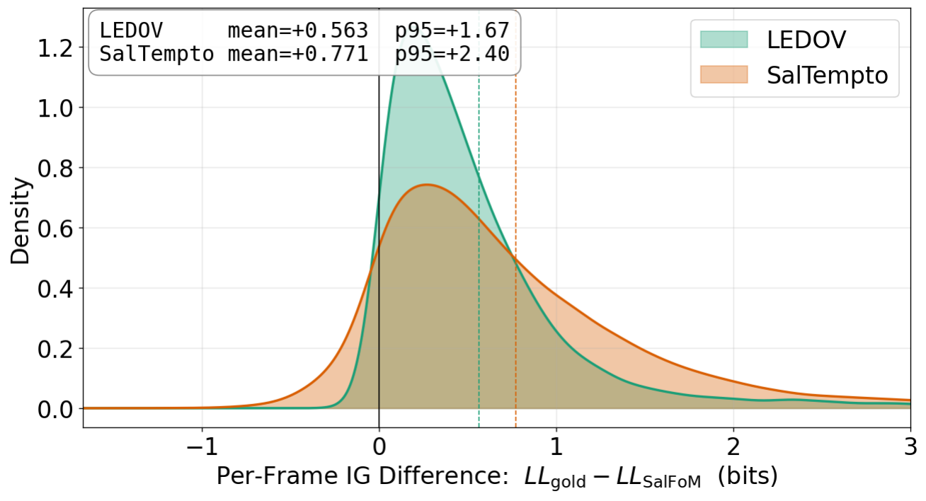
SalTempto leaves more residual information to be explained than LEDOV. Figure 2a plots the per-frame information-gain residual on each dataset. The mean per-frame residual is larger on SalTempto (+0.77 bit vs +0.56 bit); the 95th-percentile residual is approximately 44 % larger (+2.4 bit vs +1.67 bit). The shape difference is informative: LEDOV has a high peak and a long thin right tail (skewness +4.72), consistent with the “mostly easy frames plus occasional outliers” pattern that Tangemann et al. described. SalTempto is broader and less skewed (+2.40), with difficulty distributed across frames rather than concentrated in outliers.

Observed gaze behaviours. What kinds of stimulus content drive the residual on SalTempto? Tangemann et al. (2020) reported, by visual inspection of static-baseline failure cases on LEDOV, that temporal effects on gaze placement exist but are rare and uncaptured by deep models. Their analysis identified three recurring patterns: interactions between objects, where gaze concentrates at the interaction point rather than on the objects (e.g., a child feeding a giraffe); suddenly appearing objects, which strongly attract gaze (e.g., text appearing on screen); and movements of objects, where gaze tracks motion-bearing locations (e.g., a gymnast’s torso during a swinging exercise).
We sample a few high-residual clips from the right tail of Figure 2a. Apart from the known failure modes discussed above (interactions, sudden object appearance, movement), which still show up, through manual examination of SalTempto videos and gaze recordings, we observe and characterise three additional visual behaviours that current models often fail to capture.
Object permanence despite occlusion (Churchland et al., 2003; Balaban et al., 2024). Subject gaze persists on a transiently occluded target, while models redistribute to currently visible salient content (Figure 3). The corresponding video shows a workshop scene with an iron rod clamped on a vice. As observed by Tangemann et al. (2020), the interaction point of the rod and vice accounts for a majority of the gaze density over a period of time. The figure shows that the exact region remains interesting for observers even when the point of interaction becomes occluded by a moving arm.
Scene inertia (Carmi and Itti, 2006; Wang et al., 2012). Subject gaze persists across an abrupt scene-composition shift while models reattend to the new visual content. This can happen if there is a sudden change of the scene itself or if a sudden action occurs in an ongoing scene that causes a large displacement of a salient object in a short time, as shown in Figure 5. The corresponding video cuts between two stances of a fencing bout: pre-cut, the fencers stand on the right of the frame; post-cut, within just a few frames, they have shifted to the starting positions. While human observers take a few seconds to reset their attention targets, models shift their predictions unrealistically fast.
Anticipatory saccades (Vig et al., 2011; Tonn et al., 2025). Subject gaze leads moving content, pre-attending to where it will arrive, while models track it from current visual evidence and capture only the trailing component (Figure 4). The corresponding video shows a badminton smash with the shuttle moving rapidly right-to-left across the frame after the strike. Subject fixations form a smooth trail spanning the shuttle’s trajectory, with the leading edge of observer trajectories leading it (the anticipatory component). The models concentrate predicted gaze on the players and miss the moving shuttle that subjects find most salient.


5 Discussion
Architectural targets. Each observed behaviour (§4) points at a structured prior that the current model class does not reliably encode: object permanence (occlusion), scene-state continuity (scene inertia), and event continuity (anticipatory saccades). Architectural implementations of each prior exist in adjacent fields, for example, memory-integrated architectures (Park et al., 2025; Ravi et al., 2024), object state tracking (Ravi et al., 2024; Carion et al., 2025; Tokmakov et al., 2021), scene-cut detection (Souček and Lokoč, 2020; Zhu et al., 2023), motion estimation (Teed and Deng, 2020) and trajectory extrapolation (Zhao et al., 2024) modules. These have not been applied to video saliency prediction widely, and open an interesting avenue for future research directions.
Self-inclusion in the gold standard. The gold-standard mixture for each dataset includes SalFoM fine-tuned on that dataset as a mixture component. Substituting other panel models for this component changes neither the model ranking nor the cross-dataset contrast, and SalFoM recovers the smallest fraction of the headroom under its own ceiling (App. B). In general a future model more capable than SalFoM can be substituted in for a better gold standard. The gold standard is, and should be, an improving target: as models improve, more of the available gaze information becomes measurable, raising the bar for the amount of information models are expected to explain.
Early-frame protocol. Subjects’ gaze is centre-anchored for the first 15 frames following the fixation cross (Figure 6). Tangemann et al. (2020) excluded these frames; we retain them because they are part of the empirical centerbias and excluding them would create a baseline-vs-model mismatch. We observe consistent model failure on the center-focused viewing pattern at video onset, but do not pool it with the previously discussed viewing behaviours, as this is specific to recording setups. We still show it as a failure case (Figure 6): the data is readily available during training, so models should capture this behaviour.
Limitations. SalTempto is sourced from an action dataset, so its dynamics are those of human activity in the foreground, with camera motion and scene cuts as they occur in web video; content whose dynamics come from no acting agent is not targeted by the selection criterion, which limits the scope of the conclusions drawn. The evaluation splits comprise 10 validation and 10 test videos; at one minute each they carry more viewing time than LEDOV’s evaluation splits (§3.1) and span a broader range of content (§3.1), and the static and temporal intervals do not overlap on either dataset (Table 2). The dataset-level comparison is against LEDOV alone, for the reasons in §2.
6 Conclusion
Tangemann et al. (2020) diagnosed that LEDOV’s predictable gaze structure is largely recoverable by a static baseline, and observed in passing that the temporal effects which do exist are rare and uncaptured by contemporary models. We have shown that the diagnosis remains valid under a panel of recent state-of-the-art architectures: a fine-tuned static probe still recovers more than half of LEDOV’s headroom above centerbias, and the strongest current temporal model improves on it only modestly. SalTempto is the stand-alone benchmark with greater dynamism this diagnosis implies. The same fine-tuned static probe recovers only a small fraction of SalTempto’s headroom; even with dataset-specific fine-tuning, the strongest temporal model in the panel leaves nearly half of it unexplained, and shows a heavier-tailed per-frame residual than on LEDOV. LEDOV is still useful for ranking general saliency architectures, but it is weak as a diagnostic for temporal attention - the key aspect that is supposed to distinguish the video saliency problem from static image saliency modelling. SalTempto is a more temporally demanding benchmark that reveals both gains from current temporal models and substantial remaining failures. The three gaze behaviours we describe (object permanence despite occlusion, scene inertia, and anticipatory saccades), alongside the failure modes categorised by Tangemann et al. (2020), characterise where the remaining gap lies; how often each occurs and how much of the residual each explains requires a dedicated annotation study, which we leave to future work. Our results indicate that the field has measured architectural progress against a benchmark that does not measurably require temporal reasoning, and we provide a setting on which the field can begin to address this mismatch directly.
AI use statement
In this work, we used generative AI tools for some of the tasks with required disclosure: coding agents were used in part to assist with implementation, mainly in setting up coding environments and automating replication of public baselines from GitHub; the remaining required-disclosure tasks (synthetic data generation, theoretical or mathematical claims and proofs, translation, qualitative or thematic data analysis) are not applicable to this work. Additionally, we used generative AI tools for tasks with recommended disclosure: to edit the research paper to improve readability, to draft parts of the paper from author-written notes, to create or edit software code (LaTeX and figure- and table-formatting scripts). We have reviewed all AI-assisted work: all AI-assisted text was read and revised by the authors, all AI-assisted code was checked by the authors. All numbers were taken from evaluation script outputs and not fabricated or hallucinated by AI agents. We take responsibility for the final content of this work, including text, claims or artifacts produced with the aid of generative AI. AI agents were not used to propose or refine hypotheses, to design or provide feedback on the research methodology or experiments, to clean or reformat the dataset, or to interpret results.
Ethics statement
SalTempto involves research with human subjects. The eye-tracking experiment was approved by the institutional ethics board (institution withheld for anonymity), and informed consent was obtained from all participants prior to recording (§3.1). The procedures (chin-rest stabilisation, 5-point calibration, drift checks between blocks, self-paced breaks) follow standard psychophysics practice with no known risks beyond brief screen viewing. Released gaze data are anonymised. The stimuli are derived from the publicly available HACS-Segments dataset (Zhao et al., 2019); SalTempto will be released as a hosted benchmark on acceptance (§3.1). Video saliency prediction is a non-generative, non-decision-making research area, and we do not see a direct pathway to misuse.
Reproducibility statement
Section 3 documents the stimulus selection criteria, the recording apparatus and protocol, the train/validation/test splits, the model panel with the provenance of each released checkpoint, the fine-tuning protocol and its compute footprint, and the construction of the centerbias and gold-standard mixture. App. A defines the IGE metric and reports LL, IGE, KLD, CC, SIM, AUC and NSS for every model on every (dataset, split) pair, so that any number in the main text can be traced to a table cell. App. C specifies how the dataset-level dynamism metrics are computed. An anonymised repository (https://huggingface.co/datasets/bethgelab/video_saliency) holds the training and validation videos with the underlying raw 500 Hz gaze trajectories and per-frame binned positions, the test videos with gaze held out, and the evaluation code; the hosted benchmark is released on acceptance (§3.1). All benchmarked architectures are evaluated from their publicly released checkpoints, cited in §3.2.
Acknowledgements
Susmit Agrawal was supported by the German Research Foundation (DFG): SFB 1233, Robust Vision: Inference Principles and Neural Mechanisms, TP C2, project number: 276693517. Julianne Verwiebe is supported by the Carl Zeiss Foundation through the project “Certification and Foundations of Safe ML Systems”. Both authors thank the International Max Planck Research School for Intelligent Systems (IMPRS-IS) for support. All authors were supported by the Tübingen AI Center.
References
- DeepGaze3.5-vl: modeling scanpaths via autoregressive token prediction. In Computer Vision – ECCV 2026, P. Favaro, Z. Kukelova, A. Maki, A. Rohrbach, K. Schindler, and F. Tombari (Eds.), Cham, pp. 242–269. External Links: ISBN 978-3-032-37271-0 Cited by: §3.1.
- Raising the ceiling: better empirical fixation densities for saliency benchmarking. External Links: 2605.03885, Link Cited by: §3.2, §3.2.
- Electrophysiology Reveals That Intuitive Physics Guides Visual Tracking and Working Memory. Open Mind 8, pp. 1425–1446. Note: _eprint: https://direct.mit.edu/opmi/article-pdf/doi/10.1162/opmi_a_00174/2483508/opmi_a_00174.pdf External Links: ISSN 2470-2986, Link, Document Cited by: §4.
- What do different evaluation metrics tell us about saliency models?. IEEE Transactions on Pattern Analysis and Machine Intelligence 41 (3), pp. 740–757. External Links: Document Cited by: §3.2.
- SAM 3: segment anything with concepts. External Links: 2511.16719, Link Cited by: §5.
- Causal saliency effects during natural vision. In Proceedings of the 2006 Symposium on Eye Tracking Research & Applications, ETRA ’06, New York, NY, USA, pp. 11–18. External Links: ISBN 1595933050, Link, Document Cited by: §4.
- Evidence for object permanence in the smooth-pursuit eye movements of monkeys.. Journal of neurophysiology 90 (4), pp. 2205–2218 (eng). External Links: ISSN 0022-3077 1522-1598, Document Cited by: §4.
- Confidence intervals in within-subject designs: A simpler solution to Loftus and Masson’s method. Tutorials in Quantitative Methods for Psychology 1 (1), pp. 42–45. External Links: Document Cited by: Table 8, Figure 1, Figure 2.
- Unified Image and Video Saliency Modeling. In European Conference on Computer Vision (ECCV), pp. 419–435. External Links: Document Cited by: §3.2.
- TinyHD: Efficient Video Saliency Prediction with Heterogeneous Decoders using Hierarchical Maps Distillation. In Proceedings of the IEEE/CVF Winter Conference on Applications of Computer Vision (WACV), pp. 2051–2060. Cited by: §3.2.
- ViNet: Pushing the Limits of Visual Modality for Audio-Visual Saliency Prediction. In 2021 IEEE/RSJ International Conference on Intelligent Robots and Systems (IROS), pp. 3520–3527. External Links: Document Cited by: §3.2.
- Predicting Video Saliency with Object-to-Motion CNN and Two-layer Convolutional LSTM. In Computer Vision – ECCV 2018, Vol. 11218, pp. 625–642. Note: arXiv:1709.06316 [cs]Comment: Jiang, Lai and Xu, Mai and Liu, Tie and Qiao, Minglang and Wang, Zulin; DeepVS: A Deep Learning Based Video Saliency Prediction Approach;The European Conference on Computer Vision (ECCV); September 2018 External Links: Link, Document Cited by: §1, §2.
- Predicting Visual Fixations. Annual Review of Vision Science 9, pp. 269–291. External Links: Document Cited by: Appendix A, §3.2, §3.2.
- Information-theoretic model comparison unifies saliency metrics. Proceedings of the National Academy of Sciences 112 (52), pp. 16054–16059 (EN). Note: Company: National Academy of Sciences Distributor: National Academy of Sciences Institution: National Academy of Sciences Label: National Academy of Sciences Publisher: Proceedings of the National Academy of Sciences External Links: Link, Document Cited by: Appendix A, §3.2.
- DeepGaze II: Reading fixations from deep features trained on object recognition. arXiv. Note: arXiv:1610.01563 [cs] External Links: Link, Document Cited by: §3.2.
- UniFormer: Unified Transformer for Efficient Spatiotemporal Representation Learning. In International Conference on Learning Representations (ICLR), External Links: 2201.04676 Cited by: §3.2.
- Actions in the Eye: Dynamic Gaze Datasets and Learnt Saliency Models for Visual Recognition. IEEE Transactions on Pattern Analysis and Machine Intelligence 37 (7), pp. 1408–1424. External Links: ISSN 1939-3539, Link, Document Cited by: §2.
- TASED-Net: Temporally-Aggregating Spatial Encoder-Decoder Network for Video Saliency Detection. In Proceedings of the IEEE/CVF International Conference on Computer Vision (ICCV), pp. 2394–2403. Cited by: §3.2.
- Clustering of Gaze During Dynamic Scene Viewing is Predicted by Motion. Cognitive Computation 3 (1), pp. 5–24 (en). External Links: ISSN 1866-9956, 1866-9964, Link, Document Cited by: Appendix B, §2.
- SalFoM: Dynamic Saliency Prediction with Video Foundation Models. In Proceedings of the International Conference on Pattern Recognition (ICPR), External Links: 2404.03097 Cited by: §3.2.
- Confidence intervals from normalized data: A correction to Cousineau (2005). Tutorials in Quantitative Methods for Psychology 4 (2), pp. 61–64. External Links: Document Cited by: Table 8, Figure 1, Figure 2.
- VideoTitans: scalable video prediction with integrated short- and long-term memory. In The Thirty-ninth Annual Conference on Neural Information Processing Systems, External Links: Link Cited by: §5.
- SAM 2: segment anything in images and videos. arXiv preprint arXiv:2408.00714. External Links: Link Cited by: §5.
- Potsdam data set of eye movement on natural scenes (daemons). Frontiers in Psychology Volume 15 - 2024. External Links: Link, Document, ISSN 1664-1078 Cited by: §3.1.
- TransNet v2: an effective deep network architecture for fast shot transition detection. arXiv preprint arXiv:2008.04838. Cited by: §5.
- Measuring the Importance of Temporal Features in Video Saliency. In Computer Vision – ECCV 2020, A. Vedaldi, H. Bischof, T. Brox, and J. Frahm (Eds.), Cham, pp. 667–684 (en). External Links: ISBN 978-3-030-58604-1, Document Cited by: Table 1, §1, §1, §2, §2, §3.2, §4, §4, §4, §4, §5, §6.
- RAFT: Recurrent All-Pairs Field Transforms for Optical Flow. In European Conference on Computer Vision (ECCV), pp. 402–419. External Links: Document Cited by: Appendix C, §5.
- Learning to track with object permanence. 2021 IEEE/CVF International Conference on Computer Vision (ICCV), pp. 10840–10849. External Links: Link Cited by: §5.
- A gaze into the void: Anticipatory saccades toward prevented events. Attention, Perception, & Psychophysics 87 (3), pp. 848–861. External Links: ISSN 1943-393X, Link, Document Cited by: §4.
- Eye Movements Show Optimal Average Anticipation with Natural Dynamic Scenes. Cognitive Computation 3 (1), pp. 79–88. External Links: ISSN 1866-9964, Link, Document Cited by: §4.
- Temporal eye movement strategies during naturalistic viewing.. Journal of vision 12 (1), pp. 16 (eng). External Links: ISSN 1534-7362, Document Cited by: §4.
- Revisiting Video Saliency: A Large-scale Benchmark and a New Model. arXiv (en). Note: arXiv:1801.07424 [cs]Comment: CVPR2018 paper. Website: https://github.com/wenguanwang/DHF1K We have corrected some statistics of our results (baseline training setting (iii)) on UCF sports dataset External Links: Link, Document Cited by: §2.
- HACS: Human Action Clips and Segments Dataset for Recognition and Temporal Localization. arXiv. Note: arXiv:1712.09374 [cs] External Links: Link, Document Cited by: §1, §3.1, Ethics statement.
- Target-point attention transformer: a novel trajectory predict network for end-to-end autonomous driving. In 2024 IEEE Intelligent Vehicles Symposium (IV), Vol. , pp. 2325–2330. External Links: Document Cited by: §5.
- Transformer-Based Multi-Scale Feature Integration Network for Video Saliency Prediction. IEEE Transactions on Circuits and Systems for Video Technology 33 (12), pp. 7696–7707. External Links: Document Cited by: §3.2.
- AutoShot: a short video dataset and state-of-the-art shot boundary detection. In Proceedings of the IEEE/CVF Conference on Computer Vision and Pattern Recognition Workshops (CVPRW), Cited by: §5.
Appendix A Per-(dataset, split) Results
We follow the information-theoretic evaluation framework of Kümmerer et al. (2015); Kümmerer and Bethge (2023): models are scored by the log-likelihood (LL) they assign to held-out gaze. To ground LL against a known baseline, the Information Gain (IG) with respect to the dataset’s centerbias is computed as , with the gold standard’s IG defining an empirical upper bound . This allows us to quantify how much of the gap between the centerbias and the gold standard is captured by a model, through the ratio of the two quantities, defined as the Information Gain Explained (IGE). By construction and :
| (1) |
| Model | LEDOV | SalTempto | ||
|---|---|---|---|---|
| val | test | val | test | |
| DG-MR | 55.6 % | 56.4 % | 15.8 % | 10.2 % |
| SalFoM | 75.4 % | 75.2 % | 55.6 % | 61.4 % |
Table 2 reports the same quantities pooled over all evaluation videos of each dataset, with leave-one-video-out jackknife intervals.
| Dataset | Model | IG (bits) | IGE (%) | ||
|---|---|---|---|---|---|
| mean | 95 % jackknife | mean | 95 % jackknife | ||
| LEDOV | Gold standard | 2.359 | [2.210, 2.507] | 100.0 | — |
| DG-MR (static) | 1.321 | [1.170, 1.472] | 56.0 | [51.6, 60.4] | |
| SalFoM (temporal) | 1.775 | [1.631, 1.918] | 75.2 | [72.6, 77.9] | |
| Gap (SalFoM DG-MR) | 0.453 | [0.371, 0.535] | 19.2 | [15.8, 22.7] | |
| SalTempto | Gold standard | 1.864 | [1.613, 2.115] | 100.0 | — |
| DG-MR (static) | 0.243 | [0.011, 0.474] | 13.0 | [0.8, 25.2] | |
| SalFoM (temporal) | 1.090 | [0.900, 1.280] | 58.5 | [52.8, 64.1] | |
| Gap (SalFoM DG-MR) | 0.847 | [0.618, 1.077] | 45.5 | [34.7, 56.2] | |
| Method | FT | LL | IGE | KLD | CC | SIM | AUC | NSS |
|---|---|---|---|---|---|---|---|---|
| Best gold standard (adaptive 4-mix SalFoM) | — | 3.1943 | 100.0 % | 0.7102 | 0.8175 | 0.5591 | 0.9755 | 8.5661 |
| SalFoM | ✓ | 2.3583 | 55.6 % | 1.5343 | 0.4816 | 0.3331 | 0.9147 | 3.0683 |
| SalFoM | 2.2784 | 51.4 % | 1.5807 | 0.4702 | 0.3321 | 0.9140 | 2.9986 | |
| TMFI-Net | 2.0917 | 41.5 % | 1.8402 | 0.4363 | 0.3091 | 0.9045 | 2.7174 | |
| ViNet-E | 1.9527 | 34.1 % | 1.7652 | 0.4016 | 0.2738 | 0.8955 | 2.4230 | |
| ViNet-A | 1.9407 | 33.4 % | 1.7607 | 0.4011 | 0.2820 | 0.8955 | 2.4431 | |
| UniformerSal-SpatioTemporal | 1.9134 | 32.0 % | 1.5251 | 0.4655 | 0.3597 | 0.8983 | 2.4587 | |
| TASED-Net | 1.8595 | 29.1 % | 1.8248 | 0.3910 | 0.2705 | 0.8896 | 2.4073 | |
| TinyHD-single | 1.8314 | 27.6 % | 1.8690 | 0.3884 | 0.2548 | 0.8924 | 2.3710 | |
| UniformerSal-Spatial | 1.8210 | 27.1 % | 1.6108 | 0.4526 | 0.3562 | 0.8976 | 2.4483 | |
| ViNet-S | 1.7833 | 25.1 % | 1.8620 | 0.3719 | 0.2626 | 0.8863 | 2.2508 | |
| TinyHD-multi | 1.7260 | 22.0 % | 1.9339 | 0.3671 | 0.2414 | 0.8877 | 2.2273 | |
| DG-MR | ✓ | 1.6082 | 15.8 % | 2.2170 | 0.3067 | 0.2182 | 0.8719 | 2.0390 |
| UNISAL-Spatial | 1.4617 | 8.0 % | 5.9256 | 0.0485 | 0.0088 | 0.8692 | 1.8923 | |
| UNISAL-SpatioTemporal | 1.4578 | 7.8 % | 2.2547 | 0.3422 | 0.2606 | 0.8757 | 2.0333 | |
| DG-MR | 1.3235 | 0.7 % | 2.8716 | 0.2380 | 0.1705 | 0.8467 | 1.9238 | |
| CenterBias | — | 1.3110 | 0.0 % | 1.8066 | 0.3437 | 0.2527 | 0.8464 | 1.6610 |
| Method | FT | LL | IGE | KLD | CC | SIM | AUC | NSS |
|---|---|---|---|---|---|---|---|---|
| Best gold standard (adaptive 4-mix SalFoM) | — | 3.1579 | 100.0 % | 0.7496 | 0.7954 | 0.5523 | 0.9697 | 8.1241 |
| SalFoM | ✓ | 2.4462 | 61.4 % | 1.4629 | 0.4927 | 0.3500 | 0.9158 | 3.1212 |
| SalFoM | 2.3653 | 57.0 % | 1.5091 | 0.4818 | 0.3433 | 0.9125 | 3.0137 | |
| TMFI-Net | 2.1345 | 44.5 % | 1.7996 | 0.4563 | 0.3228 | 0.8995 | 2.8311 | |
| TinyHD-single | 1.9555 | 34.8 % | 1.7897 | 0.4082 | 0.2665 | 0.8915 | 2.4952 | |
| UniformerSal-Spatial | 1.9025 | 31.9 % | 1.5533 | 0.4657 | 0.3633 | 0.9002 | 2.4965 | |
| ViNet-E | 1.9025 | 31.9 % | 1.7679 | 0.3943 | 0.2798 | 0.8886 | 2.3938 | |
| TinyHD-multi | 1.8904 | 31.3 % | 1.8292 | 0.3949 | 0.2604 | 0.8891 | 2.4080 | |
| ViNet-S | 1.8196 | 27.4 % | 1.8195 | 0.3744 | 0.2761 | 0.8855 | 2.2970 | |
| UniformerSal-SpatioTemporal | 1.7750 | 25.0 % | 1.6084 | 0.4527 | 0.3531 | 0.8975 | 2.3957 | |
| TASED-Net | 1.7607 | 24.2 % | 1.8604 | 0.3810 | 0.2691 | 0.8805 | 2.3187 | |
| ViNet-A | 1.7435 | 23.3 % | 1.8420 | 0.3774 | 0.2758 | 0.8797 | 2.2815 | |
| UNISAL-Spatial | 1.5029 | 10.3 % | 5.9185 | 0.0496 | 0.0087 | 0.8706 | 1.9676 | |
| DG-MR | ✓ | 1.5016 | 10.2 % | 2.2650 | 0.2860 | 0.2076 | 0.8547 | 1.8680 |
| UNISAL-SpatioTemporal | 1.4126 | 5.4 % | 2.2780 | 0.3406 | 0.2598 | 0.8656 | 2.0571 | |
| CenterBias | — | 1.3136 | 0.0 % | 1.8003 | 0.3268 | 0.2431 | 0.8479 | 1.6369 |
| DG-MR | 1.2052 | % | 2.4810 | 0.2538 | 0.2067 | 0.8336 | 1.6875 |
| Method | FT | LL | IGE | KLD | CC | SIM | AUC | NSS |
|---|---|---|---|---|---|---|---|---|
| Best gold standard (adaptive 4-mix SalFoM) | — | 3.6948 | 100.0 % | 0.4009 | 0.8861 | 0.7117 | 0.9808 | 9.6380 |
| SalFoM | ✓ | 3.0937 | 75.4 % | 0.9234 | 0.7289 | 0.5401 | 0.9368 | 4.5045 |
| UniformerSal-SpatioTemporal | ✓† | 2.8710 | 66.2 % | 1.0990 | 0.6630 | 0.4900 | 0.9300 | 4.2670 |
| SalFoM | 2.8472 | 65.3 % | 1.0556 | 0.6919 | 0.5031 | 0.9254 | 4.2242 | |
| TMFI-Net | 2.7959 | 63.1 % | 1.0804 | 0.6855 | 0.4732 | 0.9244 | 4.0483 | |
| UniformerSal-Spatial | ✓† | 2.6471 | 57.0 % | 1.0030 | 0.6778 | 0.5353 | 0.9203 | 3.9882 |
| DG-MR | ✓† | 2.6115 | 55.6 % | 1.2254 | 0.6425 | 0.4673 | 0.9174 | 3.8552 |
| TinyHD-single | 2.5938 | 54.9 % | 1.2062 | 0.6580 | 0.4320 | 0.9153 | 3.9068 | |
| TinyHD-multi | 2.5237 | 52.0 % | 1.2511 | 0.6371 | 0.4148 | 0.9133 | 3.7798 | |
| ViNet-E | 2.2565 | 41.0 % | 1.3712 | 0.5770 | 0.4137 | 0.9017 | 3.2337 | |
| ViNet-S | 2.2284 | 39.9 % | 1.4052 | 0.5644 | 0.4159 | 0.9007 | 3.2266 | |
| ViNet-A | 2.1614 | 37.1 % | 1.4385 | 0.5645 | 0.4087 | 0.8968 | 3.2265 | |
| TASED-Net | 2.0454 | 32.4 % | 1.4792 | 0.5428 | 0.3575 | 0.8909 | 2.8951 | |
| UNISAL-Spatial | 1.9983 | 30.4 % | 1.5628 | 0.5338 | 0.3100 | 0.8958 | 2.9333 | |
| UNISAL-SpatioTemporal | 1.9836 | 29.8 % | 1.6098 | 0.5470 | 0.4107 | 0.8908 | 3.1071 | |
| CenterBias | — | 1.2560 | 0.0 % | 1.7238 | 0.3554 | 0.2925 | 0.8416 | 1.6506 |
| Method | FT | LL | IGE | KLD | CC | SIM | AUC | NSS |
|---|---|---|---|---|---|---|---|---|
| Best gold standard (adaptive 4-mix SalFoM) | — | 3.6209 | 100.0 % | 0.3955 | 0.8825 | 0.7122 | 0.9803 | 9.5950 |
| SalFoM | ✓ | 3.0524 | 75.2 % | 0.8969 | 0.7341 | 0.5372 | 0.9378 | 4.3478 |
| UniformerSal-SpatioTemporal | ✓† | 2.9056 | 68.7 % | 0.8218 | 0.7361 | 0.5766 | 0.9329 | 4.2549 |
| SalFoM | 2.8309 | 65.5 % | 1.0163 | 0.6920 | 0.5139 | 0.9288 | 4.0333 | |
| TMFI-Net | 2.7860 | 63.5 % | 1.0408 | 0.6864 | 0.4780 | 0.9280 | 3.8610 | |
| UniformerSal-Spatial | ✓† | 2.7021 | 59.8 % | 0.9206 | 0.6886 | 0.5443 | 0.9258 | 3.8798 |
| DG-MR | ✓† | 2.6241 | 56.4 % | 1.1536 | 0.6427 | 0.4748 | 0.9201 | 3.6546 |
| TinyHD-single | 2.5802 | 54.5 % | 1.1690 | 0.6472 | 0.4350 | 0.9202 | 3.6665 | |
| TinyHD-multi | 2.5678 | 54.0 % | 1.1756 | 0.6418 | 0.4284 | 0.9215 | 3.6138 | |
| ViNet-E | 2.3962 | 46.5 % | 1.2477 | 0.5859 | 0.4298 | 0.9152 | 3.1637 | |
| ViNet-S | 2.3582 | 44.8 % | 1.2868 | 0.5727 | 0.4320 | 0.9135 | 3.1447 | |
| ViNet-A | 2.3095 | 42.7 % | 1.3134 | 0.5646 | 0.4198 | 0.9113 | 3.0966 | |
| TASED-Net | 2.1679 | 36.5 % | 1.3634 | 0.5636 | 0.3760 | 0.9046 | 2.9020 | |
| UNISAL-SpatioTemporal | 2.0565 | 31.6 % | 1.5136 | 0.5431 | 0.4192 | 0.8998 | 2.9770 | |
| UNISAL-Spatial | 1.9864 | 28.6 % | 1.5255 | 0.5315 | 0.3136 | 0.9011 | 2.8260 | |
| CenterBias | — | 1.3329 | 0.0 % | 1.6527 | 0.3683 | 0.3011 | 0.8515 | 1.6875 |
Cross-dataset rank consistency. Spearman between LEDOV and SalTempto IG rankings (each model’s val and test IG pooled to a single score per dataset), computed over the full 13-model panel, is . Excluding the three models whose released checkpoints were trained on LEDOV by their original authors (DG-MR, UniformerSal-Spatial, UniformerSal-SpatioTemporal) raises Spearman to 0.83 on the 10-model zero-shot inference subset (used in Figure 2(b)).
Appendix B Control experiments
Substituting the deep component of the gold standard. Table 7 replaces the fine-tuned SalFoM component of the gold-standard mixture (§3.2) with each of the next-strongest panel models and recomputes the ceiling and the recoveries of the two fine-tuned models. The ceiling moves by at most bit, and the static-vs-temporal gap by at most points on either dataset, so the cross-dataset contrast does not depend on which model serves as the component. SalFoM recovers the smallest fraction of the headroom under the SalFoM-based ceiling on both datasets, because a stronger component raises the ceiling that every model, itself included, is measured against; the reported configuration is therefore the most demanding of the four. Note that the key metrics based on fixation coordinates (LL and IG) do not depend on the gold-standard mixture and are are directly computed based on model outputs, while IGE contains the model likelihoods as a normalizing factor across the whole panel being evaluated; there is no circularity in including the model in the gold-standard mixture.
| LEDOV | SalTempto | |||||||
|---|---|---|---|---|---|---|---|---|
| Deep component | ceiling | SalFoM | DG-MR | gap | ceiling | SalFoM | DG-MR | gap |
| SalFoM (reported) | 2.359 | 75.2 % | 56.0 % | 19.2 | 1.864 | 58.5 % | 13.0 % | 45.5 |
| UniformerSal | 2.328 | 76.2 % | 56.7 % | 19.5 | 1.831 | 59.5 % | 13.3 % | 46.3 |
| DeepGaze MR | 2.283 | 77.7 % | 57.9 % | 19.9 | 1.808 | 60.3 % | 13.4 % | 46.8 |
| TMFI-Net | 2.252 | 78.8 % | 58.7 % | 20.2 | 1.848 | 59.0 % | 13.1 % | 45.8 |
SalFoM without temporal context. To separate SalFoM’s static features from its use of temporal context, we evaluate the fine-tuned model with the target frame repeated across its full context window, so that every position in the window shows the same image and the input carries no motion (Table 8). On LEDOV the static condition still recovers 64 % of the headroom, and removing temporal context costs SalFoM 0.26 bit, 15 % of its information gain over the centerbias. On SalTempto the static condition recovers 33 %, and removing temporal context costs 0.48 bit, 44 % of its gain. The share of SalFoM’s margin over DG-MR that is attributable to temporal context is similar on both datasets (57 %), because DG-MR is also weaker on SalTempto; the contrast between the datasets lies in how much of SalFoM’s own gain depends on temporal context and in how much a static model with SalFoM’s backbone can recover. Because a repeated frame is an input the model never saw in training, the static condition is a lower bound on what such a static model could achieve. The LEDOV drop bounds this artefact from above: if the entire LEDOV drop were artefact and it were of the same size on SalTempto, at least 0.22 bit of the SalTempto drop would remain attributable to temporal information.
| Dataset | Row | IG (bits) | 95 % interval | IGE (%) |
|---|---|---|---|---|
| LEDOV | DG-MR (fine-tuned) | 1.321 | [1.254, 1.389] | 56.0 |
| SalFoM, frame repeated | 1.515 | [1.452, 1.579] | 64.3 | |
| SalFoM (fine-tuned) | 1.775 | [1.725, 1.824] | 75.2 | |
| Temporal context (SalFoM frame repeated) | 0.259 | [0.185, 0.333] | 11.0 | |
| Static features (frame repeated DG-MR) | 0.194 | [0.095, 0.293] | 8.2 | |
| SalTempto | DG-MR (fine-tuned) | 0.243 | [0.072, 0.414] | 13.0 |
| SalFoM, frame repeated | 0.609 | [0.506, 0.712] | 32.7 | |
| SalFoM (fine-tuned) | 1.090 | [0.965, 1.215] | 58.5 | |
| Temporal context (SalFoM frame repeated) | 0.481 | [0.357, 0.605] | 25.8 | |
| Static features (frame repeated DG-MR) | 0.366 | [0.159, 0.573] | 19.7 |
DIEM. On DIEM (Mital et al., 2011), evaluated zero-shot with the same pipeline on its 17 test videos, DG-MR recovers 22 % of the gold-standard headroom and SalFoM 54 %. DIEM’s gaze was recorded with audio playback and heterogeneous equipment, and its model ranking correlates only weakly with the other two datasets (Spearman with LEDOV and with SalTempto), so we treat it as a secondary check.
Appendix C Dataset-level dynamism analysis
The clearest gaze-anchored signature of within-video dispersion is the cross-frame transfer log-likelihood (LL): one frame’s gold-standard density evaluated on another frame’s fixations, averaged across within-video frame pairs (Table 9). On LEDOV, cross-frame transfer carries roughly the same predictive information as the dataset-wide centerbias: LL is vs CB bits per fixation on validation ( vs on test). This indicates that within-video gaze targets are clustered tightly enough that a frame-agnostic predictor is a reasonable estimate of where salient regions in other frames lie. On SalTempto, the same quantity drops below centerbias by over a bit: LL vs CB on validation ( vs on test). Substituting one SalTempto frame’s gold density for another’s costs 1.4 bits per fixation relative to centerbias: the marker of highly dynamic within-video gaze targets.
Cross-frame recovery as a gold-relative fraction. The cross-frame transfer LL can be recast as a fraction of the achievable per-frame predictability (gold-standard LL above the uniform spatial baseline). On LEDOV val, gold LL above uniform is 3.77 bits per fixation, so one frame’s gold density evaluated on another within-video frame recovers of the achievable per-frame log-likelihood (§1). On SalTempto val, cross-frame transfer falls below the uniform baseline (LL ), so the same fraction is non-positive: substituting one frame’s gold density for another’s actively misleads, rather than transferring usefully, necessitating models to actually track salient regions over time to make accurate predictions.
The pairwise symmetrised KL between per-frame gold-standard densities tells the same story from a different reference frame: 30 % larger on SalTempto ( vs bits validation; vs test). RAFT optical-flow magnitude (Teed and Deng, 2020) at matched evaluation resolution (long edge 512) is 2.5 larger on SalTempto (mean vs px/frame validation), further confirming high spatial dynamism, although pixel-level metrics on HACS-derived web video are partially confounded by camera shake. The dispersion of optical flow across videos is also informative: its coefficient of variation is 1.6 on LEDOV but 0.56 on SalTempto, so LEDOV’s dynamism is concentrated in a few highly dynamic videos while SalTempto’s is more uniform across the dataset, which indicates uniform dynamism rather than a few highly dynamic outlier frames. All three metrics agree on direction; the gaze-anchored cross-frame LL is the most directly diagnostic.
| Split | KL (bits) | LL (bits) | Optical flow (px/frame) |
|---|---|---|---|
| LEDOV val | |||
| LEDOV test | |||
| SalTempto val | |||
| SalTempto test |