Sphere Encoder 2
Abstract
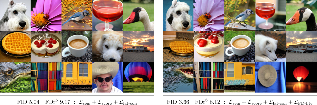
Sphere Encoder is an autoencoder that generates images by decoding random points from a high-dimensional latent sphere. We identify two limitations of the original formulation that reduce its generation quality. First, random points concentrate near the equator relative to the pole on an encoded latent, but the training rotation never reaches this region, leaving a gap that limits one-step generation. Second, training for generation with pixel-wise reconstruction loss encourages the decoder to average over plausible images, producing blurry images that lack high-frequency details. We present Sphere Encoder 2 to address both limitations, substantially improving image generation quality while maintaining the speed and simplicity of a autoencoder. Models are released at github.com/kaiyuyue/sphere2.


1 Introduction
Sphere Encoders (Yue et al., 2026; Do et al., 2026; Man et al., 2026) are simple standalone autoencoders with strong generative capabilities. They consist of an encoder that maps images into a spherical latent space, and a decoder that maps a latent vector back to an image. When trained properly, the training images cover the latent sphere with an approximately uniform distribution, enabling generation of novel images by sampling a random latent vector and passing it through the decoder. Unlike the many-step generation process used by diffusion models, sphere encoders enable fast image generation in as little as one step.
The original Sphere Encoder (Yue et al., 2026) is able to represent the ImageNet distribution, but its single-step generations are blurry (Fig. 2, top). Sharp images were obtained by iteratively passing a generated image through the encoder and decoder as many as 4 times, yet soft edges remain even after this refinement. We trace this to two causes. First, while noise is added to latent vectors during training to achieve good coverage of the sphere, the original Sphere Encoder only adds up to of noise to latents, possibly leaving some of the sphere unseen during training. Second, it trains the decoder for generation with the pixel-wise reconstruction loss, which is minimized by averaging over all plausible images and thus yields blurry outputs.
Sphere Encoder 2 fixes both issues (Fig. 2, bottom). First, we adopt a parameterization of noise that robustly adds a full of noise to latents during training, allowing the decoder to see more of the sphere during training. Second, we decouple the decoder’s task into two regimes: low-noise reconstruction, which keeps the pixel-wise loss, and high-noise generation, which drops it. In the high-noise/generative regime, we propose a new and efficient latent score matching loss. This encourages outputs to lie on the image manifold without requiring adversarial training. The result is sharp one-step generation on ImageNet (Fig. 1).
Among pixel-space generators on ImageNet, Sphere Encoder 2 achieves the best FDr6 at and the second best at with only network evaluations (NFE), whereas pixel diffusion models such as JiT (Li & He, 2026) and PixNerd (Wang et al., 2026a) take 200. This amounts to to less sampling compute in total GFLOPs. Without classifier-free guidance (CFG) (Ho & Salimans, 2022), 4 steps outperform JiT-H and one-step pMF-H (Lu et al., 2026) at both resolutions.
2 Related Work
Autoencoders (Bourlard & Kamp, 1988; Hinton & Zemel, 1993; Kingma & Welling, 2014) compress images into a latent space, but making them generate on their own is hard on complex datasets, e.g., ImageNet (Deng et al., 2009). Hierarchical VAEs such as NVAE (Vahdat & Kautz, 2020) and VDVAE (Child, 2021) deepen the latent space, yet their generation quality stays far below diffusion models (Dhariwal & Nichol, 2021) and GANs (Sauer et al., 2023). Deep VAEs (Luhman & Luhman, 2023) reach high fidelity on ImageNet only when trained inside the latent space of a pretrained tokenizer. Autoencoders then settled for the two-stage paradigm: an autoencoder only compresses, and a secondary latent diffusion Rombach et al. (2022) or autoregressive (AR) prior (Tian et al., 2024) generates. Sphere Encoder (Yue et al., 2026) revisits single-stage paradigm with a non-variational autoencoder and reaches competitive quality on ImageNet, but its generation is blurry because it treats generation as reconstruction. Sphere Encoder 2 still stays single-stage but removes the blur.
Sampling from a prior is what turns an autoencoder into a generator, and most work focuses on learning a richer prior, from mixture priors (Tomczak & Welling, 2018) to the hierarchical priors above. Spherical latents have also been explored, but either at small scale with a von Mises-Fisher posterior (Davidson et al., 2018), or with a prior still learned on top of spherical latents, autoregressive in SphereAR (Ke & Xue, 2025) and Riemannian flow matching over representation-encoder latents in RJF (Kumar & Patel, 2026). Sphere Latent Encoder (Do et al., 2026) builds on Sphere Encoder without a learned prior, but it is two-stage again and relies on a RAE decoder (Zheng et al., 2026) to reach pixels. StyleGAN (Karras et al., 2019) normalizes its input noise onto a sphere, but it does not synthesize from the sphere directly: a learned mapping network first transforms random inputs into the intermediate latent space , whose distribution is also a learned prior. Closest to our setting, (Zhao et al., 2019) decode random points on a sphere directly to pixels, but only working on MNIST and CelebA. Sphere Encoder is the first to scale sphere-to-pixel decoding to ImageNet: the decoder is trained with noise to cover the entire sphere, so no learned prior is needed.
One-step and few-step generation can be reached by two main paths. Distillation compresses a pretrained multi-step teacher into a few steps, by progressively halving steps (Salimans & Ho, 2022; Meng et al., 2023; Luhman & Luhman, 2021), straightening trajectories (Liu et al., 2022; Liu et al., 2024), enforcing consistency (Song et al., 2023; Kim et al., 2024), or matching scores or distributions (Luo et al., 2023b; Yin et al., 2024b; Yin et al., 2024a; Zhou et al., 2024), optionally with an adversarial term (Sauer et al., 2024), while from-scratch methods train one/few-step models directly, including consistency training (Song et al., 2023; Song & Dhariwal, 2024; Geng et al., 2025b; Lu & Song, 2025; Luo et al., 2023a), flow-map methods such as shortcut models, IMM, MeanFlow and its variants (Frans et al., 2025; Zhou et al., 2025; Geng et al., 2025a; Geng et al., 2026; Lu et al., 2026; Boffi et al., 2024), drifting models (Deng et al., 2026), GANs (Goodfellow et al., 2020; Brock et al., 2019; Kang et al., 2023; Huang et al., 2024; Sauer et al., 2023; Hyun et al., 2026), and Sphere Encoders (Yue et al., 2026; Do et al., 2026; Man et al., 2026). Sphere Encoder 2 is trained from scratch without distillation. One step decodes random points on the sphere directly into pixels, and each extra step loops the model by encoding, rotating, and decoding.
Distribution matching is the core of generative modeling for high-fidelity synthesis. The most effective method is the adversarial loss: a discriminator learns to tell real images from generated ones, and its gradient pushes the generator toward the data distribution (Goodfellow et al., 2020; Brock et al., 2019; Kang et al., 2023). However, adversarial training needs careful tuning and architecture design (Huang et al., 2024; Hyun et al., 2026), and its stability is a problem: BigGAN (Brock et al., 2019) collapses after a few hundred ImageNet epochs and must be stopped early, and the discriminator overfits as training proceeds (Karras et al., 2020). Distribution matching distillation (DMD) (Yin et al., 2024b) proposes an alternative: a pretrained diffusion teacher provides the real score, a second model tracks the fake score online, and their difference moves samples toward the data distribution (Wang et al., 2023; Zhou et al., 2024). The cost is the teacher: DMD requires a pretrained diffusion model of the same data or a superset of it, so it is a distillation method rather than a standalone loss for any generator. SMT (Jayashankar et al., 2025) tries to drop the teacher by learning the score of the real/fake mixture online, but operates in pixel space at or below. Concurrent work matches real and generated features of frozen encoders with MMD or optimal transport (Feng et al., 2026; Zhang et al., 2026), estimating the transport direction non-parametrically from a batch, but so far only as post-training of pretrained multi-step generators. In this work, we propose a lightweight score matching loss without a pretrained teacher. It trains two score models online from scratch, one for real and one for fake features, each a two-layer transformer following standard EDM (Karras et al., 2022), and both operate in a frozen feature space rather than pixel space, as in Projected GAN (Sauer et al., 2021), StyleGAN-T (Sauer et al., 2023), and drifting loss (Deng et al., 2026). Like a GAN loss, the score matching loss depends only on real and generated images, not on the generator itself, so in principle it can be plugged into any generator training pipeline.
3 Preliminaries: Sphere Encoder
Sphere Encoder (Yue et al., 2026) is a non-variational autoencoder that can be efficiently sampled to generate images. It consists of an encoder and a decoder . Given an input image 11 1 Bold capital letters denote matrices, and bold lower-case letters denote column vectors. The notation represents the column of a matrix , while denotes its entry in the row and column. Non-bold letters denote scalars, and denotes the vectorization of . , the encoder produces a latent , where is the number of tokens and is the feature dimension. The latent is then projected onto a global sphere by the spherify function :
| (1) |
where denotes the unit sphere in d, so lies on a sphere of radius . The decoder then maps the spherical latent back to the image space: , reconstructing the original image.
For generation, the Sphere Encoder exploits the fact that the latent space is approximately uniformly distributed on the sphere, enabling the decoder to be run with a uniform sample as input. A latent vector is chosen by spherifying a random Gaussian vector, resulting in a uniformly sampled vector on the sphere (Blum et al., 2020), and the decoder transforms it into an image:
| (2) |
3.1 Gap to the Equator
For the direct pixel generation in Eq. 2 to succeed, the decoder must handle latents that are far from any encoded seen at training time. Sphere Encoder bridges the gap between the discrete training distribution and continuous uniform distribution using a process called spherify with noise, which adds noise to a clean latent before train-time reconstruction:
| (3) |
where approximates the angle between and in high dimensions. During training, is uniformly sampled from with .
This objective leaves a mismatch between the latents seen in training and those used for generation. Specifically, on a high-dimensional sphere, almost all of the surface measure concentrates in a thin band around the equator relative to any fixed direction (Blum et al., 2020; Goldstein & Studer, 2018).
Relative to , a random point lies near the equator at . With , the decoder is never trained on the equatorial band, and the residual gap of limits its one-step generation quality. Closing the gap by setting is not an option in Eq. 3, since diverges as . This main limitation motivates a new formulation that reaches the equator exactly.
4 Sphere Encoder 2
In this section, we introduce Sphere Encoder 2, which improves generation quality by closing the gap to the equator. We explain its design choices through ablation studies.

4.1 Rotation to the Equator
We replaces additive perturbation and reprojection in Eq. 3 with an explicit rotation:
| (4) |
Since and are nearly orthogonal in high dimensions, stays on the sphere of radius , and is exactly the angle of rotation away from toward . The endpoints are well defined: recovers the clean latent, and lands on the equator (see Fig. 3).
This objective closes the gap in two ways. First, the range of now includes , so the decoder is trained on the equatorial band that one-step generation samples from. Second, although the distribution of the clean latents is not necessarily uniform, is uniform on the equatorial subsphere relative to , which is exactly the distribution of the generation latents in Eq. 2.
4.2 Still an Autoencoder
Sphere Encoder 2 keeps the simplicity of a single encoder and decoder. We use a frozen DINOv3-small (Siméoni et al., 2025) as the encoder for fast forward and high-quality generation. Each image is encoded into tokens with features per token, giving a latent size of . The latent size is shared across image resolutions of and , with patch sizes of and in pixel prediction head of the decoder, respectively.
Only the decoder , just a ViT (Dosovitskiy et al., 2021), is trained and scaled. We name models by decoder size, Sphere2-B and Sphere2-L for base and large decoders. The decoder is conditioned on the class embedding and the rotation angle , so it can behave differently along the rotation arc. Formally, the unconditional generation Eq. 2 becomes
| (5) |
We embed in the same way as diffusion timesteps (Nichol et al., 2021; Nichol & Dhariwal, 2021). The angle embedding is added to both the positional embedding of the input tokens and the class embedding used by adaLN-Zero (Peebles & Xie, 2023; Perez et al., 2018).
Alg. 1 summarizes the sampling forward. One-step generation decodes a random point on the sphere. For few-step generation, we repeatedly encode the generated image, rotate its latent toward the fixed noise direction by a fixed angle , and decode it again. Unless otherwise specified, we set in default for experiments and generate images without classifier-free guidance (CFG) (Ho & Salimans, 2022).
4.3 Angle Cutoff: Two Regimes on One Sphere
Sphere Encoder treats generation as reconstruction: the pixel-wise reconstruction loss is applied to the rotated latent along the whole arc. A pixel-space loss, however, is minimized by the mean of all plausible images, so the decoder learns to generate mean images in one-step generation.
To address this issue, we first split the rotation arc at a cutoff into two regimes, each with its own training losses. The reconstruction regime covers the low angles, , where the decoder is trained with the pixel-wise reconstruction loss:
| (6) |
where is the perceptual loss (Zhang et al., 2018b). This regime keeps the clean latent faithful, and anchors the low-angle/noise area so that rotating toward the equator starts from a semantically meaningful latent.
The generation regime covers angles near the equator. The generated images from this regime should stay semantically consistent with the input image, yet vary freely in appearance and structure. Before introducing the generation loss, we define a smooth cutoff function to weight the losses across these two regimes. The loss weight for the generation regime is a standard sigmoid centered at (Fig. 4):
| (7) |
The reconstruction regime receives . The bandwidth controls the transition width: the scale makes rise from to within of the cutoff.
4.4 Taming the Generation Regime
Reconstruction has been well studied in prior work (Yao et al., 2025; Zheng et al., 2026; Esser et al., 2024; Yue et al., 2026), and is not the focus of this work. We keep the reconstruction regime as is, without adversarial sharpening, so that any change in generation quality can be attributed to the generation losses alone. Our focus in this work is the generation regime, with the goal set above: along the rotation arc in Fig. 3, generated images should stay semantically consistent with the reconstruction while varying in appearance and structure.
4.4.1 Semantic Alignment
To preserve semantic consistency between the generation and the input , we align their logits from the ImageNet-pretrained ConvNext used in LPIPS (Zhang et al., 2018b):
| (8) |
This loss adds no cost: it shares the LPIPS perceptual loss forward in the reconstruction regime. It requires no labels, since the target is the input image itself rather than a class or a caption. In principle, a different frozen pretrained network with a global semantic embedding could also be used, such as the CLS token of CLIP (Radford et al., 2021), or SigLIP (Tschannen et al., 2025).
The cutoff angle decides how much of the arc is devoted to generation. Thus how far generated images may deviate from the input under the semantic alignment loss. We ablate this trade-off with a Sphere2-B trained on Oxford Flowers (Nilsback & Zisserman, 2008) in Fig. 5.
First, in Fig. 5 left, reconstruction quality degrades as the cutoff moves past toward the equator. This is expected: beyond , in Eq. 4, noise overwhelms the clean latent and the decoder cannot faithfully invert. Second, Fig. 5 middle and right show that 1-step and 4-step generation quality (measured by FID and FDr6, respectively) improves as moves toward the equator, peaking at . We use for all experiments by default.

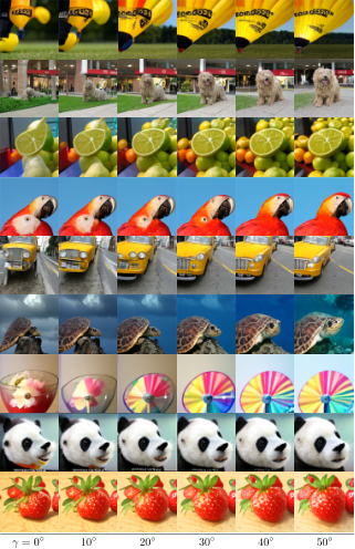
Fig. 6 visualizes the decoder outputs along the rotation arc, given the input image on the left. Below , the decoder reconstructs the input with minor variations; the softness is the intended effect of omitting adversarial training. Beyond the cutoff, generated images remain semantically consistent with the input while differing in structure and style, which is exactly the behavior the generation regime is designed for. The deviation grows with the angle, and at the output is a pure class-conditional sample, exactly the one-step generation in Eq. 2 at the equator. Current generated images are waffle-ish because the semantic alignment constrains what the decoder generates, but nothing yet drives it toward sharp, high-fidelity textures. We address this next.
4.4.2 Fidelity Improvement
Improving synthesis fidelity with a loss is a long-standing problem in generative modeling. The adversarial loss (Goodfellow et al., 2020; Brock et al., 2019; Kang et al., 2023) remains the most effective approach, but it requires careful tuning and architecture design (Huang et al., 2024; Hyun et al., 2026), and its long training suffers from stability issues (Karras et al., 2020).
We seek a simple alternative with two properties: (1) it is stable over long training on large datasets, e.g., hundreds of epochs on ImageNet; and (2) it consistently yields effective fidelity supervision as the generator improves, rather than saturating once the generator catches up. Inspired by DMD (Yin et al., 2024b; Deng et al., 2026), we propose a score matching loss that is agnostic to the generator and plugs in as a standalone loss module, in the same way as a GAN loss.

Like a GAN loss, it trains an auxiliary model online alongside the generator, but instead of a discriminator that classifies real from fake, it trains two lightweight score models, each only two transformer layers following standard EDM (Karras et al., 2022), that estimate the real and fake distributions in a frozen feature space; their difference gives the direction to move fake features toward real ones. Like a discriminator (Reed et al., 2016; Sauer et al., 2023; Zhang et al., 2018a; Kang et al., 2023; Sauer et al., 2024), the score models can be unconditional or conditioned on the class or caption.
We extract features of the input image (real) and the generated image (fake) from a frozen pretrained network , such as ConvNeXt (Woo et al., 2023) or DINO (Caron et al., 2021):
| (9) |
where indicates the layer of . have tokens and channels. and , estimated on real features only, standardize -layer features to zero mean and standard deviation , as assumed by EDM (see App. C). We drop for simplicity in the following discussion.
We build two score models, and , trained on the real features and the fake features , respectively. Both follow EDM (Karras et al., 2022) with its standard preconditioning, and each has only two transformer layers. For a feature and a noise level , the noisy feature is
| (10) |
then and learn to denoise with , where is the EDM loss weighting and follows the EDM log-normal .
To supervise the generator, we freeze both score models, evaluate them on the noisy fake feature , and take their difference, as illustrated in Fig. 7:
| (11) |
where the denominator is the denoising residual of the real score model, which normalizes the magnitude of across noise levels following DMD (Yin et al., 2024b). carries no gradient and is applied to the generator through a proxy loss:
| (12) |
where is the stop-gradient operator. Its gradient with respect to is exactly , so a step moves the fake features toward the real distribution. In practice, we score two layers of , a middle and a deep one, and balance their losses so that each contributes a gradient of equal magnitude. By default, we use the frozen ConvNeXt V2-N(ano) (Woo et al., 2023) (14.98M) as and train the score models on its middle two layers, producing the module with just total 24.16M parameters. All details of the implementation are described in App. C.
4.4.3 Latent Consistency
We also keep the latent consistency loss of Sphere Encoder (Yue et al., 2026), which encodes the generated image and matches its latent to that of the input:
| (13) |
Since is the frozen DINOv3-small, this becomes semantic alignment again, now in the latent space rather than in the logit space of . It adds one encoder forward on the generated image, which is cheap since DINOv3-small has only 29M parameters with trivial FLOPs.
4.4.4 Training Objective
In summary, Sphere Encoder 2 trains the decoder with a weighted combination of four losses:
| (14) |
5 Experiments
Tabs. 1 and 2 summarize the results of Sphere Encoder 2 on Oxford Flowers and ImageNet, respectively. For both datasets, we generate 50K images and report FDr6 (Yang et al., 2026) and gFID (Heusel et al., 2017) against the whole training set. We prioritize FDr6 over gFID, since it averages over six feature spaces rather than Inception alone, which provides a more robust evaluation of generation quality. For Sphere2 models, the sampling angle (Sec. B.4) and guidance angle (Sec. B.5) are chosen by FDr6, and gFID is reported at the same setting rather than tuned separately, since the two metrics prefer different settings. All training and evaluation details are in App. D.
On Oxford Flowers , Sphere2-B with one step and no CFG outperforms both the previous Sphere Encoder (Yue et al., 2026) and Sphere Latent Encoder (Do et al., 2026) at 4 steps with CFG, while using fewer parameters than Sphere Encoder. At this resolution, Sphere2-L improves FDr6 over Sphere2-B at every step count but has worse gFID, showing that the two metrics are not always correlated. Fig. 8 shows uncurated 4-step samples at .
| Model | Params | Guid. | NFE | FDr6 @ steps | gFID @ steps | ||||||
| 1 | 2 | 4 | 6 | 1 | 2 | 4 | 6 | ||||
| Image Size | |||||||||||
| Sphere (2026) | 948M | CFG | 10.59 | 5.44 | 3.96 | 3.92 | 25.12 | 14.08 | 11.25 | 10.63 | |
| Sphere Latent (2026) | 130M | CFG | – | – | – | – | – | 12.22 | 8.61 | 7.85 | |
| Sphere2-B | 159M | – | 2.67 | 2.23 | 2.17 | 2.19 | 7.62 | 7.45 | 7.50 | 7.55 | |
| Sphere2-L | 487M | – | 2.19 | 1.85 | 1.82 | 1.83 | 9.36 | 8.33 | 7.98 | 7.93 | |
| Image Size | |||||||||||
| Sphere2-B | 161M | – | 4.86 | 4.18 | 4.08 | 4.10 | 9.47 | 8.83 | 8.49 | 8.32 | |
| Sphere2-L | 489M | – | 4.22 | 3.67 | 3.60 | 3.61 | 9.56 | 8.34 | 7.70 | 7.59 | |

On ImageNet, Tab. 2 compares Sphere Encoder 2 with latent-space and pixel-space generators. Since Sphere Encoder 2 generates in pixel space, we mainly focus on pixel-space baselines: PixNerd (Wang et al., 2026a), JiT (Li & He, 2026), Drift (Deng et al., 2026), and pMF (Lu et al., 2026), covering both one-step and many-step generation.
At without CFG, Sphere2-B at 1 NFE is on par with JiT-B (14.53 vs. 15.78) and pMF-B (14.53 vs. 13.83), and at 4 NFE it outperforms JiT-L (8.58 vs. 10.73). Sphere2-L at 4 NFE reaches 5.77, better than JiT-H (7.66) and pMF-H (6.87), and second only to PixNerd (5.01), which uses more sampling compute. The same ordering holds at . Figs. 11, 12 and 13 show uncurated samples of Sphere2-L at 4, 2 and 1 steps without CFG, side by side with RAE-DiT-XL/2 ( NFE), JiT-L ( NFE) and pMF-L (1 NFE), respectively.
While Sphere2 leads on FDr6, its gFID is higher than that of other models. We attribute the gap to the feature space rather than the loss: matches real and fake distributions only in ConvNeXt V2-N features, and the match carries over to the other five modern spaces of FDr6 (Tab. A11) but not to the old Inception space. We investigate this in Sec. B.1 and train a second group of Sphere2 models with an FD-lite loss that mitigates this problem, marked by † in Tab. 2; Sphere2 models without the mark are trained without it. gFID drops for every model, and FDr6 improves in most settings, almost entirely through its FID term; the other five feature spaces do not move much.
| Model | Params | Guid. | Total GFLOPs | |||||
| GFLOPs | NFE | FDr6 | gFID | FDr6 | gFID | |||
| Latent space | ||||||||
| SiT-XL/2 (2024) | 675M | CFG | 119 | 8.44 | 2.06 | – | 2.62 | |
| SiT-XL/2 + REPA (2025) | 675M | CFG | 119 | 5.45 | 1.42 | – | 2.08 | |
| LightningDiT-XL/2 (2025) | 675M | CFG | 119 | 4.57 | 1.35 | – | – | |
| DDT-XL/2 (2026b) | 675M | CFG | 119 | 5.70 | 1.26 | – | 1.28 | |
| RAE-DiT-XL/2 (2026) | 839M | AG | 146 | 3.26 | 1.13 | 2.74 | 1.13 | |
| MAR-L (2024) | 478M | CFG | 129 | 6.68 | 1.80 | – | – | |
| MAR-H | 942M | CFG | 252 | 5.61 | 1.56 | – | – | |
| Sphere Latent-XL (2026) | 675M | CFG | 230 | – | 2.11 | – | – | |
| GAT-XL/2 (2026) | 602M | – | 119 | 1 | 9.26 | 2.06 | – | – |
| Drift-L (2026) | 463M | CFG∗ | 87 | 10.92 | 1.53 | – | – | |
| iMF-XL (2026) | 610M | CFG∗ | 174 | 8.39 | 1.82 | – | – | |
| iMF-XL | 610M | CFG∗ | 174 | 7.48 | 1.61 | – | – | |
| Pixel space | ||||||||
| PixNerd-XL (2026a) | 700M | CFG | 106 | 5.01 | 2.10 | 5.68 | 2.84 | |
| JiT-B (2026) | 131M | CFG | 25 | 15.78 | 3.66 | 16.31 | 4.19 | |
| JiT-L | 459M | CFG | 88 | 10.73 | 2.36 | 11.35 | 2.53 | |
| JiT-H | 953M | CFG | 182 | 7.66 | 1.86 | 8.66 | 1.94 | |
| Sphere-XL (2026) | 1.3B | CFG | 977 | 10.44 | 4.02 | – | – | |
| Drift-L | 465M | CFG∗ | 87 | 10.51 | 1.43 | – | – | |
| pMF-B (2026) | 118M | CFG∗ | 66 | 13.83 | 3.15 | 14.26 | 3.63 | |
| pMF-L | 410M | CFG∗ | 117 | 9.09 | 2.72 | 9.96 | 2.75 | |
| pMF-H | 935M | CFG∗ | 271 | 6.87 | 2.29 | 8.24 | 2.48 | |
| – | 22 | 14.53 | 5.20 | 15.17 | 5.88 | |||
| – | 22 | 8.58 | 4.89 | 9.35 | 6.04 | |||
| Sphere2-B | 161M | CFG | 22 | 7.83 | 7.00 | 8.61 | 7.94 | |
| – | 115 | 11.96 | 8.59 | 13.52 | 10.46 | |||
| – | 115 | 5.77 | 4.19 | 6.35 | 5.83 | |||
| Sphere2-L | 487M | CFG | 115 | 5.46 | 5.38 | 6.27 | 7.10 | |
| – | 22 | 12.76 | 3.43 | 13.91 | 3.85 | |||
| – | 22 | 7.95 | 3.07 | 8.49 | 2.92 | |||
| Sphere2-B† | 161M | CFG | 22 | 6.91 | 3.90 | 7.82 | 4.47 | |
| – | 115 | 13.97 | 5.14 | 11.65 | 3.69 | |||
| – | 115 | 5.14 | 2.44 | 6.60 | 3.02 | |||
| Sphere2-L† | 487M | CFG | 115 | 4.92 | 2.86 | 5.99 | 3.53 | |
Fig. 9 plots generation quality against sampling compute for the pixel-space models. Without CFG, Sphere2-B sits below Drift-L and pMF-B/L at almost the same compute, and below JiT-B/L at far less compute, i.e., better FDr6 for equal or fewer GFLOPs. Sphere2-L without CFG likewise sits below pMF-H and JiT-H. Tab. 3 compares the sampling speed of the large models at on a single H100, and adds RAE-DiT-XL/2, the latent diffusion model with the best FDr6 at this resolution in Tab. 2. For sampling 50K images at batch size 16, Sphere2-L with CFG is faster than JiT-L and faster than RAE-DiT-XL/2.
| Model | Sampler | Guid. | bsz | img/s | NFE | ms/NFE | 50K imgs (min) |
|---|---|---|---|---|---|---|---|
| Sphere2-L | loop 1 | – | 1 | 53.4 | 1 | 18.7 | 16 |
| loop 2 | CFG | 1 | 14.5 | 4 + 2 enc. | 17.3 | 58 | |
| loop 4 | CFG | 1 | 6.1 | 8 + 6 enc. | 20.7 | 137 | |
| loop 1 | – | 16 | 424.8 | 1 | 2.4 | 2 | |
| loop 2 | CFG | 16 | 145.4 | 4 + 2 enc. | 1.7 | 6 | |
| loop 4 | CFG | 16 | 62.8 | 8 + 6 enc. | 2.0 | 14 | |
| JiT-L/32 | Heun 50 | CFG | 1 | 0.5 | 198 | 10.3 | 1666 |
| Heun 50 | CFG | 16 | 4.5 | 198 | 1.1 | 185 | |
| pMF-L/32 | MeanFlow 1 | CFG∗ | 1 | 42.9 | 1 | 23.3 | 20 |
| MeanFlow 1 | CFG∗ | 16 | 157.7 | 1 | 6.3 | 6 | |
| RAE-DiT-XL/2 | Euler 49 | AG | 1 | 0.6 | 49 + 49 guide | 30.8 | 1389 |
| Euler 49 | AG | 16 | 0.9 | 49 + 49 guide | 22.1 | 926 |
6 Conclusion
Sphere Encoders are an emerging paradigm with progress from several teams (Do et al., 2026; Man et al., 2026), generating images with few steps and low compute. Sphere Encoder 2 takes this paradigm a step further, matching the image quality of more expensive diffusion models while keeping that simplicity and speed. It closes the gap to the equator with an explicit rotation, and splits the rotation arc into reconstruction and generation regimes on the same sphere. The generation regime is trained with a simple objective: semantic alignment and latent consistency keep generated images semantically faithful to the input but structurally different, and a lightweight score matching loss sharpens them without adversarial training. Several other families also targeted one-step generation from scratch, including consistency models, MeanFlow and its variants, drifting models, and GANs. Sphere Encoder 2 adds a complementary path to this landscape by bringing the autoencoder back as a generator in its own right and could be a viable candidate for one/few-step generation.

Acknowledgments
This work was supported by the NSF TRAILS Institute (2229885), and Coefficient Giving. This material is based upon work supported by the U.S. Department of Energy, Office of Science, Office of Advanced Scientific Computing Research under the Advancements in AI for Science program. This research used resources from the Argonne Leadership Computing Facility, a U.S. DOE Office of Science user facility at Argonne National Laboratory, which is supported by the Office of Science of the U.S. DOE under Contract No. DE-AC02-06CH11357.
Prepared by LLNL under Contract DE-AC52-07NA27344 and supported by the LLNL-LDRD Program under Project No. 24-ERD-010 (LLNL-PROC-2025006). This manuscript has been authored by Lawrence Livermore National Security, LLC under Contract No. DE-AC52-07NA27344 with the U.S. Department of Energy. The United States Government retains, and the publisher, by accepting the article for publication, acknowledges that the United States Government retains a non-exclusive, paid-up, irrevocable, world-wide license to publish or reproduce the published form of this manuscript, or allow others to do so, for United States Government purposes.


Appendix
Appendix A Interpolation
Fig. A14 shows class interpolation: . The random point is fixed in Eq. 5 and interpolate five points between two class embeddings by spherical linear interpolation (slerp).

Fig. A15 interpolates from images outside ImageNet. The input is looped under an ImageNet class starting from , then Alg. 1 carries it toward target class . At , in the reconstruction regime, the decoder reconstructs the input from its clean latent. The reconstruction shows the waffle-like texture seen in Fig. 6, which is expected since this regime omits adversarial sharpening. At , in the generation regime, the output is sharper and drifts toward the ImageNet manifold. Each further refinement step moves it closer to the target class.

Appendix B Ablation Studies
B.1 Distribution Shift
matches the fake and real distributions in one feature space, ConvNeXt V2-N. As Sec. 5 notes, the match carries over to the five modern spaces of FDr6 but not to the old Inception space of gFID, where the statistics of generated images drift away from those of real images. This is a mirror image of the metric paradox in FDr6 (Yang et al., 2026): most generators beat gFID but not the eye, while ours satisfies the modern feature spaces but not gFID. Ideally, we could learn a feature space specific to ImageNet as drifting models do (Deng et al., 2026), or add score models in the Inception space, but both are expensive and cumbersome. We seek a simple and cheap alternative.
To pin the statistics in place, we borrow an idea from FD loss (Yang et al., 2026) and add a Fréchet distance term on frozen features as a regularizer:
| (A15) |
where and is the Fréchet distance (Heusel et al., 2017) between real and generated features from the frozen extractor . Each term is normalized by its own detached value, so every extractor contributes a gradient of unit scale. The mean and covariance of real and fake features are tracked with exponential moving averages (EMA) online, and is computed between them. We use three small extractors: Inception, our encoder (DINOv3-small, 29M), and our score feature extractor (ConvNeXt V2-N, 16M). The latter two are already run for and , so adds one Inception forward and almost no compute.
| Steps | gFID | FDr6 | FDr6 per feature space | ||||||
|---|---|---|---|---|---|---|---|---|---|
| Incep. | ConvNeXt | DINOv2 | MAE | SigLIP | CLIP | ||||
| Sphere2-B | |||||||||
| - | 5.20 | 14.53 | 3.49 | 2.99 | 13.18 | 15.08 | 28.01 | 24.42 | |
| 1 | ✓ | 3.43 | 12.76 | 2.30 | 2.59 | 11.55 | 13.64 | 24.41 | 22.03 |
| - | 4.72 | 9.48 | 3.17 | 2.67 | 8.83 | 10.80 | 16.09 | 15.35 | |
| 2 | ✓ | 2.69 | 8.43 | 1.81 | 2.36 | 7.43 | 9.62 | 14.83 | 14.51 |
| - | 4.89 | 8.58 | 3.28 | 3.35 | 7.87 | 10.05 | 13.51 | 13.41 | |
| 4 | ✓ | 3.07 | 7.95 | 2.06 | 3.39 | 6.87 | 8.82 | 13.38 | 13.19 |
| Sphere2-L | |||||||||
| - | 8.59 | 11.96 | 5.76 | 2.49 | 9.18 | 13.54 | 21.29 | 19.48 | |
| 1 | ✓ | 5.14 | 13.97 | 3.45 | 3.11 | 9.01 | 14.65 | 29.71 | 23.89 |
| - | 5.77 | 6.42 | 3.88 | 1.78 | 5.43 | 7.39 | 9.62 | 10.41 | |
| 2 | ✓ | 3.13 | 5.92 | 2.10 | 1.70 | 4.68 | 6.97 | 9.75 | 10.31 |
| - | 4.19 | 5.77 | 2.81 | 2.69 | 5.00 | 6.56 | 8.50 | 9.05 | |
| 4 | ✓ | 2.44 | 5.14 | 1.64 | 2.05 | 4.15 | 6.01 | 8.16 | 8.86 |
Where the drift is. We train Sphere2-B and Sphere2-L on ImageNet with and without for 100 epochs from the same initial start, and report FDr6 in each feature space in Tab. A4. The Inception space is where the regularizer acts: its FDr drops by – for both models at every step count (Incep. column in Tab. A4), which is the gFID improvement in Tab. 2. The other five modern spaces move far less, mostly by single digits, confirming that the drift is specific to the decade-old Inception space rather than a general mismatch.
Model size matters. Sphere2-B benefits in every space at every step count. Sphere2-L benefits at 2 and 4 steps, but at 1 step its overall FDr6 gets worse by : the Inception term improves as before, but ConvNeXt, MAE, SigLIP and CLIP all degrade (Fig. A16, right). We read this as a capacity effect. The smaller decoder has slack to satisfy the extra constraint, while the larger decoder, which already matches the modern spaces closely without the regularizer, trades some one-step fidelity in those spaces for the Inception match. Multi-step sampling recovers the loss, since each refinement step re-encodes the image and pulls it back toward the real manifold.
Invisible to the eye.
Fig. A17 compares generations with and without from Sphere2-B, the model it affects more.
The two sets are visually indistinguishable22
2
We release Sphere2 checkpoints trained with and without in our repo for readers’ own FDr
.
, yet the loss aligns their feature statistics with those of real data in the space where gFID lives.
A good metric for image generation is still an open problem, and we hope our results on ImageNet encourage more work on it.
If a model is judged by human preference or prompt-following benchmarks rather than gFID, as text-to-image models commonly are, we believe is unnecessary and can be dropped.
Relation to FD loss. We call ours because it differs from the original FD loss (Yang et al., 2026) in purpose, and as a result in cost. The original is a post-training objective: it is the only loss applied to a pretrained multi-step generator, and its job is to repurpose the generator for one-step generation, which visibly and dramatically improves one-step quality. Ours is a regularizer. It runs alongside our other three losses throughout training with a small weight of , and only keeps the statistics of already plausible samples from drifting particularly in the Inception space. Being a regularizer rather than the main objective, it does not need the heavy extractors of the original, Inception, SigLIP-so400M and MAE-Large, and reuses the two we already run in our loss functions.


B.2 Angle Conditioning
asks the decoder to cover the real distribution rather than collapse onto its mean. We hypothesize that an angle-blind decoder hedges toward the mean, since it cannot tell latents at different angles apart. Sec. B.2 ablates conditioning the decoder on – finding our hypothesis is correct. Angle conditioning effectively improves metrics, so we keep it by default.
| cond | FDr6 | gFID | ||||
|---|---|---|---|---|---|---|
| 1 | 2 | 4 | 1 | 2 | 4 | |
| - | 4.00 | 3.21 | 3.23 | 14.02 | 12.09 | 11.95 |
| ✓ | 3.92 | 3.14 | 3.04 | 10.29 | 8.24 | 7.51 |
B.3 Angle Distribution in Training
Diffusion models commonly concentrate training samples in the high-noise region, via a noise-level (Li & He, 2026) or timestep shift (Esser et al., 2024). Sphere Latent Encoder (Do et al., 2026) likewise found that concentrating samples at high-angle noise improves generation. One might expect Sphere Encoder 2 to benefit from more training at high angles as well, especially since its decoder is conditioned on . To test this expectation, we train a Sphere2-B on Oxford Flowers and control the sampling density of during training with a single parameter by drawing it from a rational curve:
| (A16) |
where sets the shape of the curve (Fig. A20 left). Setting gives uniform sampling. A positive concentrates samples near the equator, and a negative near the pole. Fig. A20 middle and right tell a different story from common practice.
Uniform sampling () gives the best 1-step gFID, and the best FDr6 at every step count. Concentrating samples near the equator () buys only a marginal gain in multi-step gFID at . We attribute this to the angle cutoff: each regime already receives a loss tailored to it, so the decoder no longer needs an uneven sampling density to prioritize the generation. We therefore use uniform sampling by default, as the simplest and most effective choice.
B.4 Sampling Angle at Inference

Since the decoder is conditioned on the angle , we investigate sampling properties at different angles. We sweep from to in 5-degree increments for one-step generation with Sphere2-B trained on ImageNet . Fig. A21 shows that the sampling angle controls the diversity of generated images. With , the generated images are almost the same, which is expected: the decoder sees only the pure noise in Eq. 4 without any reference information from the input image during training. Thus, the decoder collapses to the mean of all plausible images in the class. With , the decoder sees a mixture of the clean latent and the noise during training, so it starts to generate images with more diversity. Fig. A22 quantifies the effect of sampling angle on ImageNet .
For multi-step generation, we apply a dense sweep and investigate the effect of sampling angle on ImageNet and Oxford Flowers at both resolutions of and . The alpha is fixed for all intermediate steps in the loop of Alg. 1. We found the FDR6 and FID do not agree on the best for multi-step generation. For simplicity, we pick for Sphere-B and for Sphere-L to report the main results in Tabs. 2 and 1, in order to prioritize FDr6 over FID.
B.5 Spherical CFG
Classic CFG (Ho & Salimans, 2022) linearly extrapolates from the unconditional prediction to the conditional one, which would push a latent off the sphere. We instead guide on the sphere with a rotation. From the same noise , we follow two parallel arcs of Alg. 1: a conditional arc with class and an unconditional arc with the null class . Following common practice, the null class is learned during training by dropping the class embedding to with probability . At each refinement step, we encode both generated images into latents and , and rotate away from along their great circle by a fixed guidance angle :
| (A17) |
The guided latent stays on the sphere at angle from , and replaces in the rotation toward the noise in Eq. 4.33 3 When and are parallel or antiparallel (), no rotation plane is defined, and we keep . This never occurs in practice, since the two arcs decode different images in the high-dimensional latent space. Unlike a guidance scale, fixes the step on the sphere regardless of how far apart the two arcs are, and recovers Alg. 1. The unconditional arc is never guided and continues from its own latent ; if it were decoded from , the two arcs would merge after one step and leave nothing to guide against. Since guidance acts on the refinement steps, it requires , and one-step generation stays unguided. Alg. 2 summarizes the sampling procedure.
| Model | Steps | Metric | Guidance angle , | Guidance angle , | |||||||||||||||
|---|---|---|---|---|---|---|---|---|---|---|---|---|---|---|---|---|---|---|---|
| Sphere2-B | 2 | FDr6 | 9.48 | 9.03 | 8.77 | 8.63 | 8.55 | 8.55 | 8.67 | 8.89 | 10.28 | 9.85 | 9.56 | 9.45 | 9.33 | 9.26 | 9.35 | 9.52 | |
| gFID | 4.72 | 5.30 | 5.80 | 6.30 | 6.78 | 7.66 | 8.34 | 9.04 | 5.64 | 6.11 | 6.46 | 7.06 | 7.46 | 8.24 | 9.16 | 9.81 | |||
| 4 | FDr6 | 8.58 | 8.08 | 7.89 | 7.83 | 7.91 | 8.20 | 8.65 | 9.17 | 9.35 | 8.92 | 8.69 | 8.61 | 8.66 | 8.91 | 9.33 | 9.85 | ||
| gFID | 4.89 | 5.58 | 6.33 | 7.00 | 7.66 | 8.66 | 9.54 | 10.02 | 6.04 | 6.62 | 7.36 | 7.94 | 8.50 | 9.54 | 10.51 | 11.23 | |||
| Sphere2-L | 2 | FDr6 | 6.42 | 6.31 | 6.28 | 6.30 | 6.39 | 6.62 | 6.94 | 7.32 | 7.50 | 7.37 | 7.28 | 7.30 | 7.31 | 7.44 | 7.61 | 7.84 | |
| gFID | 5.77 | 6.82 | 7.82 | 8.53 | 9.25 | 10.52 | 11.53 | 12.42 | 7.59 | 8.62 | 9.35 | 10.17 | 10.74 | 11.78 | 12.51 | 13.05 | |||
| 4 | FDr6 | 5.77 | 5.46 | 5.46 | 5.57 | 5.81 | 6.39 | 7.04 | 7.89 | 6.35 | 6.27 | 6.30 | 6.45 | 6.64 | 7.04 | 7.52 | 8.11 | ||
| gFID | 4.19 | 5.38 | 6.50 | 7.39 | 8.35 | 9.82 | 10.81 | 11.85 | 5.83 | 7.10 | 8.19 | 9.02 | 9.87 | 10.93 | 11.56 | 12.30 | |||
B.6 Frozen Latent Space
Tab. A7 ablates the choice of the frozen encoder . Since the encoder runs at every sampling step, we restrict the comparison to the small and base sizes of two model families, DINOv3 (Siméoni et al., 2025) and SigLIP2 (Tschannen et al., 2025) for training and inference efficiency. The small size has latent dimension and the base size . We also test a lower-dimensional variant of each, adding a single linear layer that reduces to for small and for base. The results show: (1) DINOv3 outperforms SigLIP2 at every size, and (2) DINOv3-small with its original gives the best trade-off between quality and efficiency. We therefore use it by default.
| Encoder | Compression ratio | FDr6 | gFID | |||||
|---|---|---|---|---|---|---|---|---|
| 1 | 2 | 4 | 1 | 2 | 4 | |||
| DINOv3-small | 2 | 3.92 | 3.14 | 3.04 | 10.29 | 8.24 | 7.51 | |
| DINOv3-small | 3 | 4.53 | 3.77 | 3.61 | 17.67 | 13.64 | 12.27 | |
| DINOv3-base | 1 | 4.28 | 3.58 | 3.51 | 11.47 | 9.28 | 8.69 | |
| DINOv3-base | 2 | 5.17 | 4.48 | 4.46 | 18.18 | 15.67 | 15.78 | |
| SigLIP2-base | 1 | 5.82 | 4.37 | 4.18 | 15.15 | 13.73 | 15.15 | |
| SigLIP2-base | 2 | 4.91 | 4.25 | 4.24 | 16.32 | 13.15 | 13.07 | |
B.7 Score Feature Space
needs a frozen feature space and a choice of layers. We compare two lightweight extractors: ConvNeXt V2-N, our default, and DINO-S/8, the classic choice for GAN losses (Zheng et al., 2026). For each, we sweep which layers feed the score models in Tab. A8, using Sphere2-B. The combination of a middle layer and a deep layer gives the best enough capacity for both extractors. Adding more layers costs up to twice the parameters and helps a little.
| Feature | Layers | Params | FDr6 | gFID | ||
|---|---|---|---|---|---|---|
| 1 | 4 | 1 | 4 | |||
| DINO-S/8 | 5 11 | 25.19M | 6.16 | 4.63 | 24.86 | 17.17 |
| 3 7 11 | 37.79M | 5.95 | 4.49 | 27.23 | 17.68 | |
| 5 8 11 | 37.79M | 6.20 | 4.72 | 24.28 | 17.80 | |
| 2 5 8 11 | 50.38M | 6.48 | 5.12 | 27.20 | 20.28 | |
| ConvNeXt V2-N | 1 2 | 24.16M | 6.51 | 4.88 | 26.80 | 18.60 |
| 1 3 | 44.79M | 6.42 | 5.18 | 29.85 | 21.52 | |
B.8 Score Sigma Distribution
interleaves two procedures: training the score models and transporting the generator with them. The score models are standard EDM denoisers, trained on the noisy features of Eq. 10 with drawn from the EDM log-normal , , without clamping. For the transport in Eq. 11, we draw from a second log-normal with . Two considerations guide the choice of . First, should stay within the bulk of , so the score models are never queried at noise levels they were not trained on. Second, should lean toward small noise levels, where the score difference carries the fine detail that pushes the generator toward high-fidelity and sharp generations.
Tab. A9 sweeps with fixed, using Sphere2-B. The best is : shifted toward small and slightly narrower than , as Fig. A25 shows. Pushing further hurts. At , concentrates away from the mode of , and FDr6 becomes worse. Additionally, the ImageNet finetuned version of ConvNeXt V2-N ft-in1k provides a better feature space than the pretrained ConvNeXt V2-N fcmae on Oxford Flowers, so we use it by default for all experiments.
| Feat. | Transport | FDr6 | gFID | ||
|---|---|---|---|---|---|
| 1 | 4 | 1 | 4 | ||
| DINO-S/8 | 4.54 | 3.93 | 13.69 | 10.89 | |
| 4.57 | 3.94 | 13.35 | 10.54 | ||
| 4.61 | 3.96 | 13.19 | 10.37 | ||
| 4.97 | 4.28 | 14.46 | 11.02 | ||
| 3.82 | 3.09 | 11.40 | 8.28 | ||
| 3.92 | 3.04 | 10.29 | 7.51 | ||
| 4.81 | 3.64 | 13.50 | 9.40 | ||
| ConvNeXt V2-N ft-in1k | 6.16 | 5.04 | 15.78 | 13.90 | |
| ConvNeXt V2-N fcmae | 5.03 | 3.83 | 15.07 | 13.09 | |
| 4.92 | 3.96 | 14.00 | 12.58 | ||
| 5.15 | 4.18 | 14.74 | 12.85 | ||
| 5.48 | 4.21 | 14.37 | 13.22 | ||
Appendix C Score Matching Loss
C.1 Differentiable Augmentation
We apply differentiable augmentations (Zhao et al., 2020) to the decoder output before it is passed to the frozen feature extractor during score model training. The decoder produces images of size or , and we mainly investigate DINO-S/8 (Caron et al., 2021) and ConvNeXt V2-N(ano) (Woo et al., 2023) as the feature extractor. For DINO-S/8, instead of resizing the image to , we interpolate the positional embedding to match the image size. We use two differentiable augmentations: horizontal flip with probability 0.5, and translation with probability 1.0. The translation ratio is for both resolutions, i.e., up to 4 pixels at and 8 pixels at , with reflect padding. The translation smooths the patch boundaries. Since DINO-S/8 uses patches, a shift of up to 4 or 8 pixels is half a patch at and a full patch at , so the extractor sees the generated image at every offset relative to its patch grid.
C.2 Feature Standardization
Eq. 9 standardizes the output of each scored layer of . Since the procedure is identical for every layer, we drop the index here. The raw feature has spatial locations (ConvNeXt V2-N) or tokens (DINO-S/8) and channels. EDM (Karras et al., 2022) assumes the input has zero mean and standard deviation , so we standardize the layer feature to this scale before it enters the score models.
Given a global batch of real images, we compute the per-channel mean and second moment of the raw features,
| (A18) |
where indexes the batch and indexes the spatial locations or tokens. The two statistics are accumulated as a running average over the first 1000 training steps and then frozen. Since is frozen, they converge quickly, and freezing them keeps the standardization fixed for the rest of training. They are estimated on real features only and applied to both real and fake features. This keeps the score models blind to the distribution difference between real and fake features, which is what the transport is meant to expose.
The standardization statistics of Eq. 9 are then
| (A19) |
so that has zero mean and standard deviation in every channel. For ConvNeXt V2-N, we keep per-channel wise, because a few channels have far larger variance than the rest. This is because the Global Response Normalization (GRN) layer leaves one channel dominating the others in magnitude. Each channel’s standard deviation is floored at times the median over channels, so a nearly constant channel is not amplified. For DINO-S/8, the channels are naturally balanced, and we use a single scalar per layer, the root mean of the per-channel variances.
C.3 Transport Direction
The direction in Eq. 11 is computed per sample. Its denominator is the mean absolute denoising error of the real score model over the entries of the feature map, floored at a small constant,
| (A20) |
The floor only guards against division by a vanishing error when a sample already lies on the real manifold at this ; in practice it sits well below the typical value of . The noise level is drawn from and clamped to . Both score models are frozen here, so carries no gradient.
C.4 Transport Balance
Eq. 12 is applied to every scored layer of . In practice we average the squared error over the entries,
| (A21) |
which differs from Eq. 12 by a constant that the balance weights below absorb. Since is standardized with divisor in Eq. 9, , and the gradient reaching the generated image is
| (A22) |
Its magnitude therefore scales as
| (A23) |
All three factors of depend on the layer properties: is fixed, is known, and is estimated on the fly. For DINO-S/8, is the per-layer scalar of the feature standardization. For ConvNeXt V2-N, whose is a per-channel vector, we collapse it to the scalar . This is the effective divisor: the gradient in channel is scaled by , so its norm over channels is times the root mean square of , assuming spreads evenly across channels.
Given a target magnitude , we weight each layer by
| (A24) |
so that for every layer, and the average over the scored layers keeps the loss weight independent of how many feature layers are used. Because the regression target of Eq. A20 is detached in the proxy loss function, does not depend on , and scaling by scales its gradient by exactly , so no custom backward is needed.
Since drifts as the generator improves, we track it with a running mean over the first 1000 transport steps on Oxford Flowers and 10000 on ImageNet, and an EMA with decay afterwards. The target is set to the mean of the during those 1000 steps and then frozen. The balance thus equalizes the layers and, at the same time, holds the overall gradient magnitude at its calibrated level rather than letting it fade as the fake features approach the real ones. is clipped to as a guard against a collapsed layer taking unbounded weight.
Appendix D Implementation Details
Tab. A10 lists the architecture, training, and sampling configurations of Sphere2-B and Sphere2-L used for the Oxford Flowers results in Tab. 1 and the ImageNet results in Tab. 2. Tab. A11 and Tab. A12 list the six representation models used to compute FDr6 at and on both Oxford Flowers and ImageNet.
| Sphere2-B | Sphere2-L | |
| architecture | ||
| encoder | DINOv3-small (frozen, 29M) | |
| latent | , , | |
| decoder | ViT-B | ViT-L |
| depth | 12 | 24 |
| hidden dim | 768 | 1024 |
| heads | 12 | 16 |
| image size | 256, 512 | |
| patch size of | image_size / 16 | |
| conditioning | class and angle via adaLN-Zero | |
| params (encoder + decoder) | 161M | 487M |
| GFLOPs (single forward) | 22 | 115 |
| training | ||
| epochs | 2000 on Oxford Flowers, 300 on ImageNet | |
| warmup epochs | 10 on Oxford Flowers, 5 on ImageNet | |
| optimizer | AdamW | |
| batch size | 256 | |
| learning rate | ||
| learning rate schedule | constant | |
| weight decay | 0 | |
| ema decay | 0.99985 | |
| angle sampler | ||
| cutoff angle , bandwidth | , | |
| data augmentation | center crop, horizontal flip | |
| feature extractors for | Inception, DINOv3-small, ConvNeXt V2-Nano | |
| class dropout probability (for CFG) | 0.1 | |
| score matching loss | ||
| training start epoch | 1000 on Oxford Flowers, 100 on ImageNet | |
| transport start epoch | 1150 on Oxford Flowers, 115 on ImageNet | |
| score feature space | ConvNeXt V2-N ft-in1k (frozen, 16M), two middle layers | |
| score models | 2-layer transformers, EDM preconditioning | |
| score model hidden dim | 384 | |
| score model learning rate | , same for and | |
| score model learning rate schedule | cosine decay to | |
| score for training | log-normal , no clip | |
| score for transport | log-normal , clip | |
| transport balance | EMA , | |
| differentiable augmentation | horizontal flip , translate with pixel ratio | |
| loss weights | ||
| 1.0 | ||
| 1.0 | ||
| 1.0 | ||
| 0.1 | ||
| 0.1 | ||
| sampling | ||
| sampling angle | ||
| guidance angle | ||
| Model | timm identifier | Arch. | Dim | Input | Objective | Pooling |
|---|---|---|---|---|---|---|
| Inception-v3 (Szegedy et al., 2016) | inception_v3 (torch-fidelity) | CNN | 2048 | 299 | supervised | global avg pool |
| ConvNeXt-v2 (Woo et al., 2023) | convnextv2_base.fcmae_ft_in22k_in1k | CNN | 1024 | 224 | self-supervised | global avg pool |
| MAE (He et al., 2022) | vit_large_patch16_224.mae | ViT | 1024 | 224 | reconstructive | CLS token |
| DINOv2 (Oquab et al., 2024) | vit_large_patch14_dinov2.lvd142m | ViT | 1024 | 256 | contrastive | CLS token |
| SigLIP2 (Tschannen et al., 2025) | vit_so400m_patch16_siglip_256.v2_webli | ViT | 1152 | 224 | vision-language | CLS token |
| CLIP (Radford et al., 2021) | vit_large_patch14_clip_224.openai | ViT | 1024 | 256 | vision-language | CLS token |
| Model | timm identifier | Arch. | Dim | Input | Objective | Pooling |
|---|---|---|---|---|---|---|
| Inception-v3 (Szegedy et al., 2016) | inception_v3 (torch-fidelity) | CNN | 2048 | 299 | supervised | global avg pool |
| ConvNeXt-v2 (Woo et al., 2023) | convnextv2_base.fcmae_ft_in22k_in1k_384 | CNN | 1024 | 384 | self-supervised | global avg pool |
| MAE (He et al., 2022) | vit_large_patch16_224.mae | ViT | 1024 | 224 | reconstructive | CLS token |
| DINOv2 (Oquab et al., 2024) | vit_large_patch14_dinov2.lvd142m | ViT | 1024 | 518 | contrastive | CLS token |
| SigLIP2 (Tschannen et al., 2025) | vit_so400m_patch16_siglip_512.v2_webli | ViT | 1152 | 512 | vision-language | CLS token |
| CLIP (Radford et al., 2021) | vit_large_patch14_clip_336.openai | ViT | 1024 | 336 | vision-language | CLS token |
References
- Blum et al. (2020) Avrim Blum, John Hopcroft, and Ravindran Kannan. Foundations of data science. Cambridge University Press, 2020.
- Boffi et al. (2024) Nicholas M Boffi, Michael S Albergo, and Eric Vanden-Eijnden. Flow map matching with stochastic interpolants: A mathematical framework for consistency models. TMLR, 2024.
- Bourlard & Kamp (1988) Hervé Bourlard and Yves Kamp. Auto-association by multilayer perceptrons and singular value decomposition. Biological cybernetics, 1988.
- Brock et al. (2019) Andrew Brock, Jeff Donahue, and Karen Simonyan. Large scale gan training for high fidelity natural image synthesis. In ICLR, 2019.
- Caron et al. (2021) Mathilde Caron, Hugo Touvron, Ishan Misra, Hervé Jégou, Julien Mairal, Piotr Bojanowski, and Armand Joulin. Emerging properties in self-supervised vision transformers. In ICCV, 2021.
- Child (2021) Rewon Child. Very deep vaes generalize autoregressive models and can outperform them on images. In ICLR, 2021.
- Davidson et al. (2018) Tim R Davidson, Luca Falorsi, Nicola De Cao, Thomas Kipf, and Jakub M Tomczak. Hyperspherical variational auto-encoders. In UAI, 2018.
- Deng et al. (2009) Jia Deng, Wei Dong, Richard Socher, Li-Jia Li, Kai Li, and Li Fei-Fei. Imagenet: A large-scale hierarchical image database. In CVPR, 2009.
- Deng et al. (2026) Mingyang Deng, He Li, Tianhong Li, Yilun Du, and Kaiming He. Generative modeling via drifting. arXiv preprint arXiv:2602.04770, 2026.
- Dhariwal & Nichol (2021) Prafulla Dhariwal and Alexander Nichol. Diffusion models beat gans on image synthesis. In NeurIPS, 2021.
- Do et al. (2026) Tung Do, Thuan Hoang Nguyen, and Hao Li. Efficient image synthesis with sphere latent encoder. arXiv preprint arXiv:2605.15592, 2026.
- Dosovitskiy et al. (2021) Alexey Dosovitskiy, Lucas Beyer, Alexander Kolesnikov, Dirk Weissenborn, Xiaohua Zhai, Thomas Unterthiner, Mostafa Dehghani, Matthias Minderer, Georg Heigold, Sylvain Gelly, et al. An image is worth 16x16 words: Transformers for image recognition at scale. In ICLR, 2021.
- Esser et al. (2024) Patrick Esser, Sumith Kulal, Andreas Blattmann, Rahim Entezari, Jonas Müller, Harry Saini, Yam Levi, Dominik Lorenz, Axel Sauer, Frederic Boesel, et al. Scaling rectified flow transformers for high-resolution image synthesis. In ICML, 2024.
- Feng et al. (2026) Lan Feng, Wuyang Li, Eloi Zablocki, Matthieu Cord, and Alexandre Alahi. Representation distribution matching for one-step visual generation. arXiv preprint arXiv:2607.02375, 2026.
- Frans et al. (2025) Kevin Frans, Danijar Hafner, Sergey Levine, and Pieter Abbeel. One step diffusion via shortcut models. In ICLR, 2025.
- Geng et al. (2025a) Zhengyang Geng, Mingyang Deng, Xingjian Bai, J Zico Kolter, and Kaiming He. Mean flows for one-step generative modeling. In NeurIPS, 2025a.
- Geng et al. (2025b) Zhengyang Geng, Ashwini Pokle, William Luo, Justin Lin, and J Zico Kolter. Consistency models made easy. In ICLR, 2025b.
- Geng et al. (2026) Zhengyang Geng, Yiyang Lu, Zongze Wu, Eli Shechtman, J Zico Kolter, and Kaiming He. Improved mean flows: On the challenges of fastforward generative models. In CVPR, 2026.
- Goldstein & Studer (2018) Tom Goldstein and Christoph Studer. Phasemax: Convex phase retrieval via basis pursuit. IEEE Transactions on Information Theory, 2018.
- Goodfellow et al. (2020) Ian Goodfellow, Jean Pouget-Abadie, Mehdi Mirza, Bing Xu, David Warde-Farley, Sherjil Ozair, Aaron Courville, and Yoshua Bengio. Generative adversarial networks. Communications of the ACM, 2020.
- He et al. (2022) Kaiming He, Xinlei Chen, Saining Xie, Yanghao Li, Piotr Dollár, and Ross Girshick. Masked autoencoders are scalable vision learners. In CVPR, 2022.
- Heusel et al. (2017) Martin Heusel, Hubert Ramsauer, Thomas Unterthiner, Bernhard Nessler, and Sepp Hochreiter. Gans trained by a two time-scale update rule converge to a local nash equilibrium. In NeurIPS, 2017.
- Hinton & Zemel (1993) Geoffrey E Hinton and Richard Zemel. Autoencoders, minimum description length and helmholtz free energy. In NeurIPS, 1993.
- Ho & Salimans (2022) Jonathan Ho and Tim Salimans. Classifier-free diffusion guidance. arXiv preprint arXiv:2207.12598, 2022.
- Huang et al. (2024) Yiwen Huang, Aaron Gokaslan, Volodymyr Kuleshov, and James Tompkin. The gan is dead; long live the gan! a modern gan baseline. In NeurIPS, 2024.
- Hyun et al. (2026) Sangeek Hyun, MinKyu Lee, and Jae-Pil Heo. Scalable gans with transformers. In ICML, 2026.
- Jayashankar et al. (2025) Tejas Jayashankar, Jongha Jon Ryu, and Gregory W Wornell. Score-of-mixture training: One-step generative model training made simple via score estimation of mixture distributions. In ICML, 2025.
- Kang et al. (2023) Minguk Kang, Jun-Yan Zhu, Richard Zhang, Jaesik Park, Eli Shechtman, Sylvain Paris, and Taesung Park. Scaling up gans for text-to-image synthesis. In CVPR, 2023.
- Karras et al. (2019) Tero Karras, Samuli Laine, and Timo Aila. A style-based generator architecture for generative adversarial networks. In CVPR, 2019.
- Karras et al. (2020) Tero Karras, Miika Aittala, Janne Hellsten, Samuli Laine, Jaakko Lehtinen, and Timo Aila. Training generative adversarial networks with limited data. In NeurIPS, 2020.
- Karras et al. (2022) Tero Karras, Miika Aittala, Timo Aila, and Samuli Laine. Elucidating the design space of diffusion-based generative models. In NeurIPS, 2022.
- Karras et al. (2024) Tero Karras, Miika Aittala, Tuomas Kynkäänniemi, Jaakko Lehtinen, Timo Aila, and Samuli Laine. Guiding a diffusion model with a bad version of itself. In NeurIPS, 2024.
- Ke & Xue (2025) Guolin Ke and Hui Xue. Hyperspherical latents improve continuous-token autoregressive generation. arXiv preprint arXiv:2509.24335, 2025.
- Kim et al. (2024) Dongjun Kim, Chieh-Hsin Lai, WeiHsiang Liao, Naoki Murata, Yuhta Takida, Toshimitsu Uesaka, Yutong He, Yuki Mitsufuji, and Stefano Ermon. Consistency trajectory models: Learning probability flow ode trajectory of diffusion. In ICLR, 2024.
- Kingma & Welling (2014) Diederik P Kingma and Max Welling. Auto-encoding variational bayes. In ICLR, 2014.
- Kumar & Patel (2026) Amandeep Kumar and Vishal M Patel. Learning on the manifold: Unlocking standard diffusion transformers with representation encoders. arXiv preprint arXiv:2602.10099, 2026.
- Li & He (2026) Tianhong Li and Kaiming He. Back to basics: Let denoising generative models denoise. In CVPR, 2026.
- Li et al. (2024) Tianhong Li, Yonglong Tian, He Li, Mingyang Deng, and Kaiming He. Autoregressive image generation without vector quantization. In NeurIPS, 2024.
- Liu et al. (2022) Xingchao Liu, Chengyue Gong, and Qiang Liu. Flow straight and fast: Learning to generate and transfer data with rectified flow. arXiv preprint arXiv:2209.03003, 2022.
- Liu et al. (2024) Xingchao Liu, Xiwen Zhang, Jianzhu Ma, Jian Peng, et al. Instaflow: One step is enough for high-quality diffusion-based text-to-image generation. In ICLR, 2024.
- Lu & Song (2025) Cheng Lu and Yang Song. Simplifying, stabilizing and scaling continuous-time consistency models. In ICLR, 2025.
- Lu et al. (2026) Yiyang Lu, Susie Lu, Qiao Sun, Hanhong Zhao, Zhicheng Jiang, Xianbang Wang, Tianhong Li, Zhengyang Geng, and Kaiming He. One-step latent-free image generation with pixel mean flows. arXiv preprint arXiv:2601.22158, 2026.
- Luhman & Luhman (2021) Eric Luhman and Troy Luhman. Knowledge distillation in iterative generative models for improved sampling speed. arXiv preprint arXiv:2101.02388, 2021.
- Luhman & Luhman (2023) Troy Luhman and Eric Luhman. High fidelity image synthesis with deep vaes in latent space. arXiv preprint arXiv:2303.13714, 2023.
- Luo et al. (2023a) Simian Luo, Yiqin Tan, Longbo Huang, Jian Li, and Hang Zhao. Latent consistency models: Synthesizing high-resolution images with few-step inference. arXiv preprint arXiv:2310.04378, 2023a.
- Luo et al. (2023b) Weijian Luo, Tianyang Hu, Shifeng Zhang, Jiacheng Sun, Zhenguo Li, and Zhihua Zhang. Diff-instruct: A universal approach for transferring knowledge from pre-trained diffusion models. In NeurIPS, 2023b.
- Ma et al. (2024) Nanye Ma, Mark Goldstein, Michael S Albergo, Nicholas M Boffi, Eric Vanden-Eijnden, and Saining Xie. Sit: Exploring flow and diffusion-based generative models with scalable interpolant transformers. In ECCV, 2024.
- Man et al. (2026) Sean Man, Ron Raphaeli, Matan Kleiner, and Or Ronai. SP3: Spherical priors for plug-and-play restoration. In NeurIPS, 2026.
- Meng et al. (2023) Chenlin Meng, Robin Rombach, Ruiqi Gao, Diederik Kingma, Stefano Ermon, Jonathan Ho, and Tim Salimans. On distillation of guided diffusion models. In CVPR, 2023.
- Nichol et al. (2021) Alex Nichol, Prafulla Dhariwal, Aditya Ramesh, Pranav Shyam, Pamela Mishkin, Bob McGrew, Ilya Sutskever, and Mark Chen. Glide: Towards photorealistic image generation and editing with text-guided diffusion models. arXiv preprint arXiv:2112.10741, 2021.
- Nichol & Dhariwal (2021) Alexander Quinn Nichol and Prafulla Dhariwal. Improved denoising diffusion probabilistic models. In ICML, 2021.
- Nilsback & Zisserman (2008) Maria-Elena Nilsback and Andrew Zisserman. Automated flower classification over a large number of classes. In Conference on computer vision, graphics & image processing, 2008.
- Oquab et al. (2024) Maxime Oquab, Timothée Darcet, Théo Moutakanni, Huy Vo, Marc Szafraniec, Vasil Khalidov, Pierre Fernandez, Daniel Haziza, Francisco Massa, Alaaeldin El-Nouby, et al. DINOv2: Learning robust visual features without supervision. TMLR, 2024.
- Peebles & Xie (2023) William Peebles and Saining Xie. Scalable diffusion models with transformers. In ICCV, 2023.
- Perez et al. (2018) Ethan Perez, Florian Strub, Harm De Vries, Vincent Dumoulin, and Aaron Courville. Film: Visual reasoning with a general conditioning layer. In AAAI, 2018.
- Radford et al. (2021) Alec Radford, Jong Wook Kim, Chris Hallacy, Aditya Ramesh, Gabriel Goh, Sandhini Agarwal, Girish Sastry, Amanda Askell, Pamela Mishkin, Jack Clark, et al. Learning transferable visual models from natural language supervision. In ICML, 2021.
- Reed et al. (2016) Scott Reed, Zeynep Akata, Xinchen Yan, Lajanugen Logeswaran, Bernt Schiele, and Honglak Lee. Generative adversarial text to image synthesis. In ICML, 2016.
- Rombach et al. (2022) Robin Rombach, Andreas Blattmann, Dominik Lorenz, Patrick Esser, and Björn Ommer. High-resolution image synthesis with latent diffusion models. In CVPR, 2022.
- Salimans & Ho (2022) Tim Salimans and Jonathan Ho. Progressive distillation for fast sampling of diffusion models. In ICLR, 2022.
- Sauer et al. (2021) Axel Sauer, Kashyap Chitta, Jens Müller, and Andreas Geiger. Projected gans converge faster. In NeurIPS, 2021.
- Sauer et al. (2023) Axel Sauer, Tero Karras, Samuli Laine, Andreas Geiger, and Timo Aila. Stylegan-t: Unlocking the power of gans for fast large-scale text-to-image synthesis. In ICML, 2023.
- Sauer et al. (2024) Axel Sauer, Dominik Lorenz, Andreas Blattmann, and Robin Rombach. Adversarial diffusion distillation. In ECCV, 2024.
- Siméoni et al. (2025) Oriane Siméoni, Huy V Vo, Maximilian Seitzer, Federico Baldassarre, Maxime Oquab, Cijo Jose, Vasil Khalidov, Marc Szafraniec, Seungeun Yi, Michaël Ramamonjisoa, et al. Dinov3. arXiv preprint arXiv:2508.10104, 2025.
- Song & Dhariwal (2024) Yang Song and Prafulla Dhariwal. Improved techniques for training consistency models. In ICLR, 2024.
- Song et al. (2023) Yang Song, Prafulla Dhariwal, Mark Chen, and Ilya Sutskever. Consistency models. In ICML, 2023.
- Szegedy et al. (2016) Christian Szegedy, Vincent Vanhoucke, Sergey Ioffe, Jon Shlens, and Zbigniew Wojna. Rethinking the inception architecture for computer vision. In CVPR, 2016.
- Tian et al. (2024) Keyu Tian, Yi Jiang, Zehuan Yuan, Bingyue Peng, and Liwei Wang. Visual autoregressive modeling: Scalable image generation via next-scale prediction. In NeurIPS, 2024.
- Tomczak & Welling (2018) Jakub Tomczak and Max Welling. Vae with a vampprior. In Conference on artificial intelligence and statistics, 2018.
- Tschannen et al. (2025) Michael Tschannen, Alexey Gritsenko, Xiao Wang, Muhammad Ferjad Naeem, Ibrahim Alabdulmohsin, Nikhil Parthasarathy, Talfan Evans, Lucas Beyer, Ye Xia, Basil Mustafa, et al. Siglip 2: Multilingual vision-language encoders with improved semantic understanding, localization, and dense features. arXiv preprint arXiv:2502.14786, 2025.
- Vahdat & Kautz (2020) Arash Vahdat and Jan Kautz. Nvae: A deep hierarchical variational autoencoder. In NeurIPS, 2020.
- Wang et al. (2026a) Shuai Wang, Ziteng Gao, Chenhui Zhu, Weilin Huang, and Limin Wang. Pixnerd: Pixel neural field diffusion. In ICLR, 2026a.
- Wang et al. (2026b) Shuai Wang, Zhi Tian, Weilin Huang, and Limin Wang. Ddt: Decoupled diffusion transformer. In CVPR, 2026b.
- Wang et al. (2023) Zhengyi Wang, Cheng Lu, Yikai Wang, Fan Bao, Chongxuan Li, Hang Su, and Jun Zhu. Prolificdreamer: High-fidelity and diverse text-to-3d generation with variational score distillation. In NeurIPS, 2023.
- Woo et al. (2023) Sanghyun Woo, Shoubhik Debnath, Ronghang Hu, Xinlei Chen, Zhuang Liu, In So Kweon, and Saining Xie. Convnext v2: Co-designing and scaling convnets with masked autoencoders. In CVPR, 2023.
- Yang et al. (2026) Jiawei Yang, Zhengyang Geng, Xuan Ju, Yonglong Tian, and Yue Wang. Representation fréchet loss for visual generation. In NeurIPS, 2026.
- Yao et al. (2025) Jingfeng Yao, Bin Yang, and Xinggang Wang. Reconstruction vs. generation: Taming optimization dilemma in latent diffusion models. In CVPR, 2025.
- Yin et al. (2024a) Tianwei Yin, Michaël Gharbi, Taesung Park, Richard Zhang, Eli Shechtman, Fredo Durand, and William T Freeman. Improved distribution matching distillation for fast image synthesis. In NeurIPS, 2024a.
- Yin et al. (2024b) Tianwei Yin, Michaël Gharbi, Richard Zhang, Eli Shechtman, Fredo Durand, William T Freeman, and Taesung Park. One-step diffusion with distribution matching distillation. In CVPR, 2024b.
- Yu et al. (2025) Sihyun Yu, Sangkyung Kwak, Huiwon Jang, Jongheon Jeong, Jonathan Huang, Jinwoo Shin, and Saining Xie. Representation alignment for generation: Training diffusion transformers is easier than you think. In ICLR, 2025.
- Yue et al. (2026) Kaiyu Yue, Menglin Jia, Ji Hou, and Tom Goldstein. Image generation with a sphere encoder. arXiv preprint arXiv:2602.15030, 2026.
- Zhang et al. (2026) Chi Zhang, Haoyang Shi, Yueyi Liu, Ruichuan An, Junkang Zhou, Chang Li, Xiuyuan Lu, Yichi Zhang, Bo Wang, Yuhang Wu, Sen Cui, and Miao Liu. Unifying distributional training for one-step visual generation. arXiv preprint arXiv:2609.35763, 2026.
- Zhang et al. (2018a) Han Zhang, Tao Xu, Hongsheng Li, Shaoting Zhang, Xiaogang Wang, Xiaolei Huang, and Dimitris N Metaxas. Stackgan++: Realistic image synthesis with stacked generative adversarial networks. TPAMI, 2018a.
- Zhang et al. (2018b) Richard Zhang, Phillip Isola, Alexei A Efros, Eli Shechtman, and Oliver Wang. The unreasonable effectiveness of deep features as a perceptual metric. In CVPR, 2018b.
- Zhao et al. (2019) Deli Zhao, Jiapeng Zhu, and Bo Zhang. Latent variables on spheres for autoencoders in high dimensions. arXiv preprint arXiv:1912.10233, 2019.
- Zhao et al. (2020) Shengyu Zhao, Zhijian Liu, Ji Lin, Jun-Yan Zhu, and Song Han. Differentiable augmentation for data-efficient gan training. In NeurIPS, 2020.
- Zheng et al. (2026) Boyang Zheng, Nanye Ma, Shengbang Tong, and Saining Xie. Diffusion transformers with representation autoencoders. In ICLR, 2026.
- Zhou et al. (2025) Linqi Zhou, Stefano Ermon, and Jiaming Song. Inductive moment matching. In ICML, 2025.
- Zhou et al. (2024) Mingyuan Zhou, Huangjie Zheng, Zhendong Wang, Mingzhang Yin, and Hai Huang. Score identity distillation: Exponentially fast distillation of pretrained diffusion models for one-step generation. In ICML, 2024.