Comparing a gradient boosting algorithm to the GOES FDC for wildfire detection
Abstract
Wildfires pose severe risks to human life, ecosystems, and property. This study presents a machine learning approach for wildfire detection from GOES ABI imagery. A CatBoost model was trained on a large dataset with thousands of ABI images and over 300,000 matching VIIRS fire detections. An evaluation on a separate dataset across five regions showed that the learned CatBoost model outperformed the operational GOES Fire Detection and Characterization (FDC) product. It achieved higher precision, recall, and F1 scores both within and outside the training area. The CatBoost model achieved F1 scores that were 0.16 to 0.38 higher than the GOES FDC in all regions. In addition, out of 51 historical fire events, the CatBoost detected 26 fires before both VIIRS and GOES FDC, compared to only six earlier detections by the GOES FDC. Importantly, the CatBoost model achieved accurate wildfire detection also during nighttime, whereas the GOES FDC obtained very low recall values, around 0.03. This study demonstrates that machine learning models may offer significant improvements over existing geostationary fire products, including higher accuracy, fewer false alarms, and earlier detection.
Keywords: CatBoost model, Fire Detection and Characterization, Early detection, Geostationary satellites, VIIRS
1 Introduction
Wildfires can have devastating impacts on the environment and pose serious threats to human life, ecosystems, and property. A recent example is the Palisades Fire, which erupted in January 2025 in Los Angeles, California, resulting in 12 fatalities, destroyed more than 6,800 structures, and burning 95 km2 of land over 24 days before being fully contained [CAL FIRE, 2025]. Given the rapid spread of such severe events, timely fire detection can help contain fires and prevent large-scale disasters. This is even more crucial nowadays, as the frequency of major disasters caused by wildfires has quadrupled from 1980 to 2023 [Cunningham et al., 2025].
A common approach to early wildfire detection is the use of satellite imagery, which provides wide-area coverage and frequent monitoring [Chuvieco et al., 2020]. Among satellite-based methods, geostationary (GEO) satellites are commonly used for wildfire detection [Barmpoutis et al., 2020]. Their orbital period matches Earth’s rotation, so they appear stationary from a fixed point on the ground and can monitor the same region every 5 to 15 minutes.
Indeed, several dedicated fire detection products were developed for GEO satellite imagery. Notable examples include the Fire Detection and Characterization (FDC) product of the American Geostationary Operational Environmental Satellite (GOES) [Schmidt, 2020], and the Fire Radiative Power (FRP-PIXEL) product of the European Meteosat Second Generation (MSG) satellite [Wooster et al., 2015]. These products are based on a combination of threshold and contextual criteria and have several known limitations. As discussed by Schmidt [2020], some fire events are visible in the 3.7 µm band before the FDC algorithm detects them. In addition, Hall et al. [2019], Hall et al. [2023] report that the FDC and FRP fire products exhibit high false-alarm rates. These findings highlight the need for fire detection algorithms with lower false-alarm rates and greater detection capabilities, particularly for small fires.
A promising approach to address this challenge is to train machine learning (ML) algorithms for GEO fire detection. ML algorithms have the potential to outperform traditional algorithms by learning fire-related complex spatial and spectral patterns from GEO satellite imagery [Yang et al., 2024]. Training a ML algorithm requires a labeled dataset consisting of multispectral imagery annotated at the pixel level as fire or non-fire. These annotations are derived from independent reference sources. Examples include high-resolution fire detections from Low Earth Orbit (LEO) satellite instruments [Zhao and Ban, 2022, Zhang et al., 2023, e.g.,], and fire records from national forest services [Jang et al., 2019, Kang et al., 2022, Kang et al., 2023, e.g.,]. After the model has been trained, given a new GEO image, its output is a binary image, indicating whether each pixel is fire or not. Finally, it is common practice to evaluate the model’s accuracy on an independent dataset that was not seen during training.
Several studies considered ML approaches for GEO fire detection. Some works used traditional ML algorithms, such as Random Forest (RF) [Jang et al., 2019, Zhang et al., 2023, Maeda and Tonooka, 2023, Liu et al., 2023], while other studies applied Deep Learning (DL) algorithms, like Convolutional Neural Networks (CNNs) [Hong et al., 2022, Hong et al., 2024, Ding et al., 2022, Zhao and Ban, 2022, Kang et al., 2022, Kang et al., 2023, Ji et al., 2023]. These studies show the potential of ML algorithms for GEO fire detection. Nevertheless, important limitations and gaps remain to be addressed.
One gap is that most of the published ML models for GEO fire detection used relatively small training and evaluation datasets, containing only a few hundred annotated fire pixels. In addition, both the training and evaluation regions covered only small-scale geographic areas. Furthermore, Most works did not assess the models’ generalization to regions outside the training areas. Another issue is that, in many studies, the trained ML models were not empirically compared with the corresponding operational GEO fire detection algorithms. Furthermore, previous studies did not assess their model performance separately on daytime and nighttime images, but rather provided its overall accuracy. Consequently, it is unclear whether these ML models truly outperform existing algorithms, particularly in terms of low false alarms and detection capability across a broad range of atmospheric conditions and over the large coverage areas of GEO satellites.
The primary goal of this study is to develop a robust ML model for GEO fire detection that outperforms the GOES FDC product in both detection accuracy and false-alarm rate. To this end, we trained and evaluated a ML fire detection method using a large annotated dataset containing more than 60,000 GOES ABI fire pixels and 1.2 million non-fire pixels. Reference labels for both training and evaluation were derived from the LEO Visible Infrared Imaging Radiometer Suite (VIIRS) active fire product. A Gradient Boosting ML fire detection algorithm was trained on this dataset and evaluated on a large, separate dataset. The evaluation dataset includes images from regions not used in training and from a different time period. Specifically, the training data are from 2022–2023, while the evaluation data are from 2024. These differences in both space and time between the training and evaluation datasets enable a comprehensive assessment of the model’s generalization capability. In addition, the model performance was compared to the GOES FDC product in terms of overall detection and daytime/nighttime detection.
2 Study area and data sources
This section describes the regions analyzed in the study and the satellite imagery acquired over them. The images were used to train and evaluate a ML model for GEO fire detection. In addition, as detailed below, a set of specific fire events was compiled to compare the ML model’s early detection capabilities with those of the GOES FDC product.
2.1 Study area
The study area encompasses several regions in the United States, Mexico, and Canada, with diverse land-cover types, including forests, wetlands, deserts, agricultural and urban areas (Figure 1). As illustrated in the figure, part of the study area was used solely for training, another solely for evaluation, and a third for both training and evaluation. Specifically, the U.S. states of Florida, Alabama, Mississippi, Louisiana, and Oklahoma, as well as the Mexican states of Chihuahua and Durango, were used for training. Texas and Georgia were used for both training and evaluation, whereas California, Oregon, Arizona, Utah, and a small region in British Columbia were used exclusively for evaluation. The size of the training area is approximately 2.1 million km2, whereas that of the evaluation region is about 2 million km2.

2.2 Data sources
The training and evaluation datasets have the same structure. Each dataset consists of VIIRS fire detections and matching GOES Advanced Baseline Imager (ABI) images acquired within a min interval. Further details on the data utilized from VIIRS and GOES ABI products are provided below.
The training dataset consists of all VIIRS fire detections in the study area throughout all of 2022 and 2023. It contains 324,502 VIIRS fire detections and 4330 corresponding GOES ABI images. The evaluation dataset contains VIIRS fire detections from selected months in 2024, see Table 1. The following paragraphs elaborate on the specific data sources used to construct the training and evaluation datasets. These include the VIIRS active fire product, GOES ABI imagery, and fire perimeter data.
| Region | Months (2024) | GOES ABI Number of images | VIIRS Number of detected fires |
| Georgia | February, March, April | 185 | 8211 |
| Texas | March, April, May | 325 | 9005 |
| California-Oregon | July, August, September | 363 | 53,259 |
| Arizona-Utah | September, October, November | 285 | 5309 |
| British Columbia | July, August, September | 115 | 1523 |
2.2.1 VIIRS active fire product
In this work, data from the VIIRS instrument onboard the Suomi National Polar-orbiting Partnership (Suomi NPP) satellite were used as a reference. Specifically, reference fire labels were derived from VIIRS active fire product VNP14IMG Collection 2 [Schroeder et al., 2014].
The VNP14IMG product has a spatial resolution of 375 m. For each fire detection (pixel), it provides its location (latitude and longitude), acquisition date and time, fire radiative power (FRP), and confidence level. Fire detections with low confidence were deemed insufficiently reliable to serve as a reference and were thus excluded from the dataset. The data were downloaded from NASA’s Level-1 and Atmosphere Archive and Distribution System Distributed Active Archive Center (LAADS DAAC)11 1 https://ladsweb.modaps.eosdis.nasa.gov, accessed on 1 February 2026.
2.2.2 GOES ABI images
Three GOES ABI products with a spatial resolution of 2 km were downloaded: (1) Multi-channel Cloud and Moisture Imagery (MCMI); (2) Clear Sky Mask (ACM); and (3) FDC. The MCMI and ACM data serve as input to the ML model, while the FDC data serves as the benchmark fire detector against which we compare our trained ML model. The MCMI provides 16-band multispectral images. The complementary ACM indicates which pixels are cloudy and was used for cloud masking. The FDC product uses a contextual algorithm based on thermal infrared bands to identify thermal anomalies. It assigns each pixel a value indicating whether it is a fire. Pixels classified as fire have a corresponding confidence category. These categories reflect the algorithm’s confidence level that the detected fire is indeed a fire [Schmidt et al., 2020]. For evaluation analysis (Section 3.4), all of the FDC confidence categories were included. For the early detection analysis (Section 4.4), the evaluation was performed twice. First, only the processed and saturated categories were used, as they have the lowest false alarm rates among the FDC categories [Hall et al., 2023]. Second, the high category was added to the previous ones. Despite its higher false-alarm rate, it was included to assess whether it enables earlier fire detection. Both GOES-16 and GOES-18 ABI products were downloaded in Continental United States (CONUS) and Pacific U.S. (PACUS) scan modes, respectively, using the GOES Python library22 2 https://pypi.org/project/GOES/, accessed on 1 February 2026 (version 3.9.23).
2.2.3 Fire perimeter data for early detection assessment
To compare the early-detection capabilities of the ML model and the GOES FDC (Section 4.4), a dataset of fire-perimeter measurements for 51 specific fire events was constructed as follows. The perimeter data was retrieved from the Wildland Fire Interagency Geospatial Services database (WFIGS)33 3 https://data-nifc.opendata.arcgis.com/datasets/nifc::wfigs-current-interagency-fire-perimeters/about, accessed on 1 February 2026. The data contains polygons representing the mapped perimeters of wildfire events across the U.S. The locations of the fire events are shown in Figure 2. Further details regarding the 51 fire events appear in Table A.1 in Appendix A.

3 Methodology
As detailed below, the construction of the ML fire detection algorithm consists of the following steps:
- (i)
Spatial assignment of VIIRS fire detections to the GOES ABI grid (Section 3.1).
- (ii)
Construction of the labeled dataset (Section 3.2).
- (iii)
ML model training (Section 3.3).
- (iv)
ML model evaluation (Section 3.4).
Code of the trained ML model and some example data are available at the author’s GitHub repository44 4 https://github.com/asafvanunu/GOES_wildfire_detection, accessed on 1 February 2026.
3.1 Assigning VIIRS fire detections to GOES ABI grid
As mentioned above, VIIRS and GOES ABI have different spatial resolutions and grid systems. Thus, to label GOES ABI pixels as fire/no fire, VIIRS fire detection pixel centroids were rasterized onto the GOES ABI fixed grid. The rasterized output is a GOES ABI grid, in which each pixel represents the number of VIIRS fire-detection centroids that intersect it. Pixels without any VIIRS fire-detection intersections were assigned a value of 0. Figure 3 illustrates the rasterize function, available in the Rasterio Python library55 5 https://rasterio.readthedocs.io/en/stable/api/rasterio.features.html, accessed on 1 February 2026 [Gillies, 2019].
The VIIRS instrument captures imagery in successive swaths known as scan lines. Due to its technical properties, there is an overlap between VIIRS pixels from adjacent scan lines. This phenomenon is commonly referred to as the bow-tie effect [Seaman et al., 2015]. Most of these duplicated pixels are removed onboard the instrument. However, residual bow-tie pixels remain and may affect the analysis. Thus, duplicated VIIRS pixels were removed using the method described by Vanunu et al. [2026].

3.2 Labeled dataset construction
Next, we describe the process to label GOES ABI pixels as fire/no fire. These steps include handling spatial misalignments between VIIRS and GOES ABI fire detections, labeling non-fire pixels, and extracting input features for the ML model. A significant challenge in constructing a labeled dataset is the frequent spatial misalignment between VIIRS fire detections and GOES ABI observations. As shown in several studies [Pestana and Lundquist, 2022, Ayala et al., 2023, Vanunu et al., 2026], there can be displacements of several kilometers between GOES ABI and VIIRS fire pixel locations. This, in turn, can significantly affect the accuracy of the trained ML model.
To ensure accurate labeling of GOES ABI fire pixels that takes into account spatial misalignments, a buffer window was applied. Specifically, let be the rasterized image. A value represents a VIIRS fire detection at ABI grid location in the rasterized output (Section 3.1). Similarly, let denote a pixel at the same location and time stamp in the GOES MCMI image. As illustrated in Figure 4, for each location with , a buffer window was applied around . Within this window, the GOES ABI pixel with the highest fire signal, quantified by the Fire Index (FI), was labeled as a fire pixel. The FI [Zhao and Ban, 2022] is the normalized ratio between the shortwave infrared (SWIR) band at 3.9 µm and the thermal infrared (TIR) band at 11.2 µm:
| (1) |
where and are the GOES ABI brightness temperatures (in Kelvin) at 3.9 µm and 11.2 µm bands, respectively. The 3.9 µm band is sensitive to fires, while the 11.2 µm band is not. High FI values are associated with active fires and thus considered a reliable indicator of fire presence[Zhao and Ban, 2022].
Note that applying a (square or circular) buffer window around a GEO fire detection is common practice in evaluating the accuracy of GEO fire products [Freeborn et al., 2014, Wickramasinghe et al., 2020, Xu et al., 2017, Xu et al., 2021, Hall et al., 2019, Hall et al., 2023, e.g.,]. If a LEO fire detection falls within this window, the GEO fire detection is considered a valid fire. Here, in contrast, the buffer window is placed around the VIIRS fire detection, and the purpose is different: to label GEO pixels as fires while accounting for and correcting potential misalignments.
For non-fire pixel labeling, from each GOES ABI image, 500 pixels that satisfy the following two requirements were selected: (1) It cannot intersect a labeled fire pixel in a window. (2) It cannot be within a window of any pixel with in the corresponding image . These requirements ensure non-fire pixels are distant from fire-labeled pixels.

For each labeled pixel (fire or non-fire), the values of all its 16 bands as well as its FI value were extracted. Additionally, a window was applied around each pixel to obtain its spatial context. From the pixels within the window (excluding the center pixel), five statistics were computed for all 17 bands (including the FI): mean, median, minimum, maximum, and standard deviation. Pixels flagged as cloud-covered by the ACM product were excluded from these calculations. If all of the neighboring pixels were flagged as clouds, a fill value of -999 was assigned. The number of contextual features is . In total, there are 102 features (17 band values at the center pixel and 85 contextual features).
To exclude small fires that the GOES ABI struggles to detect, two filtering criteria were applied to the fire-labeled pixels: (1) The number of VIIRS fire detections in the window around the center pixel at the corresponding matrix was required to be ; and (2) The FI value was required to be .
Next, the class imbalance between fire and non-fire pixels was addressed. Satellite-based wildfire detection datasets are highly imbalanced, as non-fire pixels greatly outnumber fire pixels. To mitigate this, a 1:20 ratio of fire to non-fire pixels was applied. This ratio was chosen to preserve sufficient background pixels while preventing the non-fire class from dominating the model training. Ratios of 1:10 and 1:30 were also tested. Although the 1:30 ratio achieved similar precision, the 1:20 ratio was selected because its better F1 score. In summary, the training dataset contained 202,000 fire-labeled and 2,165,000 non-fire-labeled GOES ABI pixels. After the filtering criteria were applied, 65,877 fire-labeled and 1,317,540 non-fire-labeled pixels remained.
3.3 Model training
In this study, a CatBoost [Prokhorenkova et al., 2018] algorithm was trained to detect fires. CatBoost (Categorical Boosting) is a gradient-boosting method that builds an ensemble of decision trees. Each tree is trained to correct the errors made by the earlier trees.
CatBoost can process different types of input features without complex pre-processing. It handles numerical values and categorical variables in a unified way. Unlike traditional gradient boosting frameworks, CatBoost incorporates specific algorithmic innovations to improve accuracy and generalization. These include: (1) ordered boosting, a technique that shuffles training data to prevent the model from memorizing the target (’target leakage’); (2) native handling of categorical variables, which avoids the need for complex pre-processing of non-numerical data; and (3) oblivious decision trees, a balanced tree structure that acts as a regularizer to prevent overfitting and significantly speeds up prediction times. CatBoost has been widely applied across a variety of domains [Hancock and Khoshgoftaar, 2020], including remote sensing [Zhang et al., 2022]. The training dataset was randomly divided into 80% for training and 20% for validation. Further details regarding the CatBoost model training are provided in Appendix B.
3.4 Accuracy evaluation of a fire detection algorithm
To evaluate the accuracy of a fire detection algorithm, spatial misalignments between GOES ABI and VIIRS observations were considered. Similar to Section 3.2, let denote that at ABI pixel location the fire detection algorithm predicted a fire. A pixel with is classified as a True Positive (TP) if there is at least one within a window around . Otherwise, the pixel is considered a False Positive (FP). A False Negative (FN) pixel is defined as follows. If the window around does not contain a model fire detection, then the pixel is defined as FN. The calculation of FN, TP, and FP with a window is illustrated in Figure 5. The red pixels are the model fire detections. In contrast, the pink pixels are rasterized VIIRS fire detections.

The accuracy of a fire detection algorithm is evaluated by its recall, precision, and F1 scores. These are standard metrics for classifier assessment. In the context of fire detection, recall is the proportion of true fire pixels that the algorithm correctly identifies as fires. Precision is the ratio of correctly detected fire pixels to the total number of flagged fire pixels by the algorithm. The harmonic mean of precision and recall is the F1 score. All three metrics range from 0 to 1, where higher values indicate improved accuracy.
To compute recall, precision, and F1, the total number of TP, FP, and FN pixels was summed across the entire image dataset. We denote these quantities by , and . Accordingly, let denote a pair of GEO/rasterized VIIRS images, and let represent the index of a single image. For each image , we denote by , , and the number of pixels in that image classified as TP, FP, and FN, respectively. The totals were then calculated:
Based on these totals, the precision, recall, and F1 metrics were calculated:
| Recall | (2) | |||
| Precision | (3) | |||
| F1 | (4) |
4 Results
This section presents the empirical evaluation results of the CatBoost model trained as described in section 3.3. In particular, we compare its performance with that of the GOES FDC in terms of accuracy, early-detection capabilities and ability to detect small fires.
4.1 CatBoost performance against the GOES FDC
Figure 6a-c shows the recall, precision, and F1 scores, respectively, for the CatBoost model and the GOES FDC product across all five evaluation regions (Georgia, Texas, California-Oregon, Arizona-Utah and British Columbia). The results show that the CatBoost model outperformed the GOES FDC product across all regions and evaluation metrics. It achieved lower false alarm rates and equal or higher detection rates. In California–Oregon, Arizona-Utah and British Columbia, CatBoost performed better in recall, precision, and F1, regions that are not in the training dataset. This demonstrates the transferability of the trained CatBoost model to regions outside the training areas. In all regions, the CatBoost ML model achieved F1 scores that were 0.16-0.38 higher than those of the GOES FDC.

Going beyond the quantitative evaluation described above, it is instructive to look at two specific fire events, one in Texas and the other in Georgia. Figure 7 shows the CatBoost model’s predictions. The green squares of width 375 m, are fires detected by the VIIRS fire product on images of the two regions taken at matching times (up to min). The left image is of Texas on 19 March 2024 at 19:36 UTC, and the right image is of Georgia on 19 February 2024 at 18:41 UTC. CatBoost pixels are marked in red for TP, purple for FP, and blue for FN. In Texas, the FP pixel is near the TP, suggesting that proximity to the heat source may have caused misclassification. In Georgia, small fires with single VIIRS detections were missed by the model and labeled as FN.

4.2 Daytime/nighttime performance
Following the evaluation of the CatBoost model against the GOES FDC, it is important to explore how the time of day impacts detection capabilities. In this section, we compare the accuracy fire detection accuracy of the CatBoost and FDC models during the day and during the night across all study regions. The separation between day and night images was determined according to the sunrise and sunset times for each region. These times were computed based on the longitude, latitude, and date of each image using the Sunrise-Sunset API66 6 https://sunrise-sunset.org/api, accessed on 1 February 2026. Table 2 details the separation of the full evaluation dataset into daytime and nighttime images. The dataset contains a relatively balanced number of day and night images for most regions.
| Region | Daytime images | Nighttime images |
| Georgia | 101 | 84 |
| Texas | 153 | 172 |
| California-Oregon | 180 | 183 |
| Arizona-Utah | 135 | 150 |
| British Columbia | 38 | 77 |
Figure 8 shows the recall, precision, and F1 scores of the CatBoost and GOES FDC in all study regions during nighttime (Figure 8a) and during daytime (Figure 8b). During the daytime, recall and precision are higher for the CatBoost model, except for recall in California-Oregon and precision in Georgia and British Columbia, which are almost identical between the two algorithms. For the F1 score, CatBoost is higher than the FDC in all study regions during the day.
During the nighttime, in contrast, the CatBoost algorithm is significantly more accurate than the FDC. Notably, the recall score of CatBoost is significantly higher than the FDC. In fact, the FDC recall is 0 in Georgia and Texas, and it is almost 0 in the other regions. This means the FDC fails to detect almost all fires in the nighttime images of the study dataset. In Georgia, precision could not be calculated because the FDC did not detect any true or false positives across all 84 images. In Texas and Arizona-Utah, the FDC precision was higher than CatBoost because of the low number of FDC detections. There were only 13 fire detections in 172 images in Texas, while there were 4,409 GOES ABI pixels with at least one VIIRS fire detection in them. Similarly, there were only 26 fire detections in 134 images in Arizona-Utah, compared to 850 GOES ABI pixels with at least one VIIRS fire detection. For comparison, the CatBoost model in the corresponding regions had 477 and 691 fire detections, respectively. In the remaining regions, CatBoost achieves higher precision. For the nighttime, the CatBoost F1 scores were significantly higher, ranging from 0.17 to 0.69, while the FDC ranged from only 0.01 to 0.1. Overall, these results demonstrate that the GOES FDC struggles to detect fires at night, and the CatBoost model provides superior nighttime detection capabilities.

4.3 Impact of training dataset size on CatBoost performance
To demonstrate the importance of a large and diverse labeled dataset, we compared the model described in section 3.3 with the following two additional models. The first is a CatBoost model trained on a random subset of only 2,000 fire pixels and 20,000 non-fire pixels. The second model was trained on 2,000 fire pixels and 20,000 non-fire pixels drawn only from April and May.
Figure 9a-c presents precision, recall, and F1 scores, respectively, for all five models across Georgia, Texas, California-Oregon, Arizona-Utah and British Columbia. The full model, trained on 66,000 fire pixel, shows substantially higher precision in Texas, California–Oregon and Arizona-Utah than the two reduced-size models, while all models display similar precision in Georgia. Precision in Texas is 0.87 for the 66,000-pixel model, which is significantly higher than 0.72 and 0.68 achieved by the two 2,000-pixel models. In California-Oregon, precision is 0.88 for the 66,000-pixel model and 0.79 and 0.75 for the smaller models. In Arizona-Utah, the precision is 0.81 for the 66,000-pixel model, compared to 0.5 and 0.42 for the small models. These results show that small training datasets lead to higher false-alarm rates, especially when the dataset is restricted to only some months of the year.
Recall values are generally similar across models, with differences of about 0.04. The main exception is Georgia, where the April–May model produces a recall of only 0.21, compared with 0.33 and 0.35 for the 66,000-pixel and 2,000-pixel models. This result highlights the potential limitations of using a dataset that covers only a few specific months.
F1-scores are also similar across most models and regions, apart from the April–May model in Georgia and Arizona-Utah, which shows a clear drop in performance. In California–Oregon and Arizona-Utah, which were not part of the training area, the highest F1-score is achieved by the 66,000-pixel model. This indicates better transferability and generalization when the training dataset is large and diverse.
In summary, the 66,000-pixel model produces far fewer false-alarms than the reduced training size models while maintaining similar recall. Training on a small or limited dataset can lead to increased false-alarms and decreased performance in regions outside the training domain.

4.4 Early detection capability
Early fire detection is crucial for extinguishing small fires before they escalate to large and destructive wildfires. As mentioned in Section 2.2, a dataset of 51 fires with their fire perimeters was constructed to compare the early detection capabilities of the CatBoost model and the GOES FDC. First, for each fire event in the dataset, CatBoost model predictions and the corresponding FDC product were collected for all GOES ABI images acquired within the 8 hours preceding and 2 hours following the first VIIRS fire detection. Next, the images were cropped to a 10 km buffer around the fire polygon. Lastly, the time difference between the first fire detection of the CatBoost model and the GOES FDC was computed (in minutes).
Figure 10 summarizes the time difference between the CatBoost and GOES FDC for 38 fire events where both methods detected the fire before the time of the VIIRS image first detection. Figure 10a (left) shows the results using only the processed and saturated FDC categories, while Figure 10b (right) includes also the high confidence category. The x-axis shows the time difference in minutes, and the y-axis lists the fire events. In 10a, 22 fire events were first detected by CatBoost, with a mean earlier detection time of 20 min and a standard deviation of 17 min, while GOES FDC first detected only six fires. In 10b, the FDC fire detection capability improved with the addition of the high category addition. The CatBoost first detected 19 fires with a mean earlier detection time of 18 min and a standard deviation of 16 min. Here the GOES FDC first detected nine fires. For both analyses, 10 fire events were detected simultaneously by the CatBoost model and GOES FDC and were therefore labeled as "0".
A deeper examination of these results reveals several notable cases, specifically the Howell, Blue Stem, Candy Creek, and Silver King fires. For the Howell fire, CatBoost detected the event 60 minutes earlier than the GOES FDC when using only the processed and saturated categories. However, when the high category was included, the time difference became zero. In the Blue Stem fire, CatBoost initially detected the fire 55 minutes before the FDC. Yet, with the addition of the high category, the FDC detected the fire 115 minutes earlier than CatBoost. This indicates that the high category can sometimes enable the FDC to detect fires simultaneously with or earlier than the CatBoost model. Furthermore, the Candy Creek and Silver King fires were not detected at all by the FDC when restricted to the processed and saturated categories. Once the high category was added, both fires were detected by the FDC, and for the Candy Creek fire, the FDC even detected it 30 minutes earlier than CatBoost. These examples demonstrate that FDC categories with higher false alarm rates can, in certain situations, provide better early fire detection capabilities than the precessed and saturated categories.
Table 3 describes the remaining 13 fire events split into two categories: (1) The CatBoost model detected the fire and GOES FDC did not detect it before VIIRS; and (2) Neither CatBoost nor FDC detected a fire before the time of the VIIRS image.
Overall, out of 51 fire events, CatBoost detected 26 fires before both VIIRS and GOES FDC in the first analysis, and 23 in the second analysis. Ten fires were detected simultaneously by CatBoost and GOES FDC, while nine were first detected by VIIRS. GOES FDC first detected six fires in the first analysis and nine fires in the second. These results demonstrate that the CatBoost model has substantially better early detection capabilities than the GOES FDC product.

| Fire event | First fire detection | Time difference (minutes) |
| Beech | CatBoost | 300 |
| Bentley | 480 | |
| Davis | 445 | |
| Smokehouse Creek | 245 | |
| Airport | VIIRS | No CatBoost detection |
| Blue Mountain | ||
| Boise | ||
| Dry Branch | ||
| Duck Nest | ||
| Fall Branch | ||
| Fodderstack | ||
| Foote | ||
| Walker |
4.5 Fire detection probability
This section analyzes the CatBoost and GOES FDC fire detection probability as a function of the number of VIIRS fire detections within a spatial window of size around the GEO pixel predicted as fire by the corresponding method. This was done to assess the models’ sensitivity to different fire sizes. The approach presented here is similar to those conducted by Vanunu et al. [2026].
Let denote the binary image representing the output of a fire detection algorithm. A pixel value of 1 indicates a detected fire, and 0 otherwise. As described in Equation 5, for the window parameter (), the neighborhood set around pixel is defined as:
| (5) |
For different values of an integer , the total number of pixels with at least VIIRS fire detections and a model fire detection within a distance was calculated. This calculation was performed for all images in the dataset. Accordingly, for each image , let represent the corresponding rasterized VIIRS output with threshold
| (6) |
Likewise, the number of FP pixels was calculated
| (7) |
Hence, equals the total number of pixels containing at least VIIRS fire detections. The probability that in a window around each such pixel, there is a model fire detection was calculated.
| (8) |
Figure 11 shows the estimated probabilities as a function of across the five evaluation regions: Georgia (Figure 11a), Texas (Figure 11b), California-Oregon (Figure 11c), Arizona-Utah (Figure 11d), and British Columbia (Figure 11e). The x-axis represents the minimum number of VIIRS fire detections contained within a single GOES ABI pixel.
In California-Oregon, Arizona-Utah and British Columbia, the CatBoost model yields substantially higher fire-detection probabilities than those of GOES FDC. For instance, in California-Oregon at , GOES FDC has a fire probability of 0.28 while CatBoost’s is 0.46. At , the CatBoost probability is 0.78 compared to only 0.48 for GOES FDC. In Texas, the CatBoost model shows higher probabilities than GOES FDC for thresholds below . At , the GOES FDC probability exceeds that of the CatBoost model. This can be attributed to the very small sample size of only eight ABI pixels that contained ten or more VIIRS fire detections. Overall, the CatBoost model consistently achieves higher probabilities than GOES FDC across all regions, particularly in California and Oregon. Hence, in most cases, the CatBoost model is more sensitive to small fires and is more likely to detect them.

5 Discussion and conclusions
In this study, a CatBoost model was trained for wildfire detection using a large, carefully annotated dataset of GOES-16 ABI imagery. CatBoost was selected for this task because it is a modern, highly efficient gradient boosting framework that is relatively simple to train. The model was evaluated and compared to the GOES FDC product. For both training and evaluation, VIIRS fire detections served as a reference. The analysis in this study focused on prediction accuracy, early-detection capability, and fire-detection probability.
The results demonstrate that the CatBoost model consistently outperforms GOES FDC across all five regions considered in the study. It achieved higher precision, recall, and F1-scores. Recall values were relatively low for both models. This is due to the coarse spatial resolution of ABI compared to VIIRS. As a result, small fires detected by VIIRS were classified as false negatives by both the GOES FDC as well as by the CatBoost model. Despite this limitation, CatBoost achieved a higher recall than GOES FDC. The superior performance of the CatBoost model in California–Oregon, Arizona-Utah and British Columbia indicates generalization ability to regions outside the training domain. These evaluation regions feature different climatic conditions and varying satellite view angles compared to the training data. Additional daytime/nighttime evaluation between the CatBoost and the GOES FDC revealed striking differences. While CatBoost maintained reliable nighttime detection, the GOES FDC nighttime recall dropped to near zero across all regions. This highlights the CatBoost capabilities for fire detection across all day hours. In a different analysis, CatBoost models trained on smaller datasets highlighted the importance of training on a large, diverse labeled dataset for reliable detection and robust performance in regions outside the training area. Models trained on only 2,000 fire pixels exhibited substantially higher false-alarm rates and weaker transferability. These findings have important implications for operational wildfire monitoring. Accurate detection is critical for rapid response, especially in remote regions. In addition, improved GEO-based detection can bridge the temporal gap between LEO satellite overpasses, providing continuous fire monitoring.
The results are consistent with previous studies on ML-based fire detection using GEO satellites. Kang et al. [2023] trained a GEO-based deep learning fire detection model using imagery from the Japanese Himawari-8 Advanced Himawari Imager (AHI). The model was trained over regions in Asia and demonstrated improved performance compared to the operational Himawari fire product. The reported F1 scores were 0.66 and 0.50 at in situ validation sites in Asia. In addition, transferability analysis over Australia yielded an average F1 score of 0.68. These F1 score ranges are comparable to those achieved in the current study. Overall, their results showed promising potential for GEO-based ML fire-detection models applied across large geographic regions, potentially outperforming existing GEO fire products.
Despite these advancements in the Asia–Pacific region, the application of machine-learning-based fire-detection methods to the GOES-ABI platform remains limited. To date, only one study has applied machine learning to GOES-ABI-based fire detection. Zhao and Ban [2022] trained a deep learning model on GOES-ABI imagery using a relatively small dataset constructed from only four major fire events. Reported F1 scores were 0.71, 0.63, and 0.18 for the Creek, Camp, and Doctor Creek fires, respectively. Their model detected 24 of 38 fires earlier than VIIRS, comparable to the early-detection capability observed in the present results. However, their evaluation was limited to a small number of individual fire events and did not include a comparison with the operational GOES Fire Detection and Characterization product.
While Zhao and Ban [2022] demonstrated the potential of deep learning for GOES ABI fire detection, our work extends their study in several important ways. We evaluated the model across large-scale geographic regions rather than focusing on a small number of specific large fire events. In addition, we benchmark our model against the GOES FDC, and to the best of our knowledge, this study is the first to do so. We also explicitly assessed early detection relative to both VIIRS and GOES FDC. In addition, we quantified the detection probability as a function of VIIRS fire detections, an aspect that has not been extensively investigated in prior ML GEO-based fire detection studies.
Despite these contributions, it is important to note some limitations of our study. The algorithm was primarily tested in regions of the continental United States and parts of North America, and only the CONUS and PACUS scan modes were used. The model was not tested on full-disk imagery or regions such as the Amazon or Patagonia, and therefore, continental-scale transferability remains unexplored. In addition, only the CatBoost model was evaluated, and it is possible that other advanced machine learning models could yield similar results. Furthermore, the evaluation relied exclusively on VIIRS as a reference. Other LEO satellites with higher spatial resolution or in situ fire datasets were not used. Fire detections from these datasets are commonly included in the evaluation of GEO fire detection models [Hall et al., 2019, Hall et al., 2023, Li et al., 2020, e.g.,], as incorporating them can improve dataset labeling and evaluation.
Overall, this study shows that a CatBoost-based model can improve wildfire detection from GOES ABI imagery. It provides higher accuracy, lower false-alarm rates, and earlier detection than the GOES FDC product. These improvements highlight the potential of machine learning to strengthen operational wildfire monitoring and support more effective fire management and decision-making.
Funding
This work was supported by the Israel Space Agency, which is part of the Ministry of Science and Technology, Israel, under Grant 3-18142; and the Jewish National Fund (JNF) under Grant 2006/22.
Author Contributions
Conceptualization, A.V., B.N. and A.K.; methodology, A.V., B.N. and A.K.; software, A.V.; validation, A.V.; formal analysis, A.V.; investigation, A.V., B.N. and A.K.; resources, B.N. and A.K.; data curation, A.V.; writing—original draft preparation, A.V., B.N. and A.K.; writing—review and editing, A.V., B.N. and A.K.; visualization, A.V.; supervision, B.N. and A.K.; project administration, A.V.; funding acquisition, B.N. and A.K. All authors have read and agreed to the published version of the manuscript.
Disclosure statement
The authors report there are no competing interests to declare.
Data availability statement
The primary data that support the findings of this study are openly available in Zenodo at https://doi.org/10.5281/zenodo.19047285 Vanunu [2026]. Additional data are available from the corresponding author, A.K., upon reasonable request.
References
- Parallax shift in goes abi data. Journal of Operational Meteorology 11 (2), pp. 14–23. External Links: Document, ISSN 2325-6184 Cited by: §3.2.
- A review on early forest fire detection systems using optical remote sensing. Sensors 20 (22). External Links: ISSN 1424-8220, Document Cited by: §1.
- Palisades fire. Note: Accessed: 2025-06-30 External Links: Link Cited by: §1.
- Satellite remote sensing contributions to wildland fire science and management. Current Forestry Reports 6 (2), pp. 81–96. External Links: ISSN 2198-6436, Document Cited by: §1.
- Climate-linked escalation of societally disastrous wildfires. Science 390 (6768), pp. 53–58. External Links: Document Cited by: §1.
- Wildfire detection through deep learning based on himawari-8 satellites platform. International Journal of Remote Sensing 43 (13), pp. 5040–5058. External Links: Document Cited by: §1.
- Evaluating the seviri fire thermal anomaly detection algorithm across the central african republic using the modis active fire product. Remote Sensing 6 (3), pp. 1890–1917. External Links: ISSN 2072-4292, Document Cited by: §3.2.
- Rasterio documentation. MapBox: San Francisco, CA, USA 23. Cited by: §3.1.
- Geostationary active fire products validation: goes-17 abi, goes-16 abi, and himawari ahi. International Journal of Remote Sensing 44 (10), pp. 3174–3193. External Links: Document Cited by: §1, §2.2.2, §3.2, §5.
- Validation of goes-16 abi and msg seviri active fire products. International Journal of Applied Earth Observation and Geoinformation 83, pp. 101928. External Links: ISSN 1569-8432, Document Cited by: §1, §3.2, §5.
- CatBoost for big data: an interdisciplinary review. Journal of big data 7 (1), pp. 94. Cited by: §3.3.
- Active fire detection using a novel convolutional neural network based on himawari-8 satellite images. Frontiers in Environmental Science Volume 10 - 2022. External Links: Document, ISSN 2296-665X Cited by: §1.
- Near real-time monitoring of fire spots using a novel sbt-firenet based on himawari-8 satellite images. IEEE Journal of Selected Topics in Applied Earth Observations and Remote Sensing 17 (), pp. 1719–1733. External Links: Document Cited by: §1.
- Detection and monitoring of forest fires using himawari-8 geostationary satellite data in south korea. Remote Sensing 11 (3). External Links: ISSN 2072-4292, Document Cited by: §1, §1.
- Coupling physical model and deep learning for near real-time wildfire detection. IEEE Geoscience and Remote Sensing Letters 20 (), pp. 1–5. External Links: Document Cited by: §1.
- A deep learning model using geostationary satellite data for forest fire detection with reduced detection latency. GIScience & Remote Sensing 59 (1), pp. 2019–2035. External Links: Document Cited by: §1, §1.
- Toward an adaptable deep-learning model for satellite-based wildfire monitoring with consideration of environmental conditions. Remote Sensing of Environment 298, pp. 113814. External Links: ISSN 0034-4257, Document Cited by: §1, §1, §5.
- A preliminary evaluation of goes-16 active fire product using landsat-8 and viirs active fire data, and ground-based prescribed fire records. Remote Sensing of Environment 237, pp. 111600. External Links: ISSN 0034-4257, Document Cited by: §5.
- Integrating machine learning and a spatial contextual algorithm to detect wildfire from himawari-8 data in southwest china. Forests 14 (5). External Links: ISSN 1999-4907, Document Cited by: §1.
- Early stage forest fire detection from himawari-8 ahi images using a modified mod14 algorithm combined with machine learning. Sensors 23 (1). External Links: ISSN 1424-8220, Document Cited by: §1.
- Evaluating goes-16 abi surface brightness temperature observation biases over the central sierra nevada of california. Remote Sensing of Environment 281, pp. 113221. External Links: ISSN 0034-4257, Document Cited by: §3.2.
- CatBoost: unbiased boosting with categorical features. In Advances in Neural Information Processing Systems, Vol. 31, pp. . Cited by: §3.3.
- Chapter 13 - monitoring fires with the goes-r series. In The GOES-R Series, S. J. Goodman, T. J. Schmit, J. Daniels, and R. J. Redmon (Eds.), pp. 145–163. External Links: ISBN 978-0-12-814327-8, Document Cited by: §1.
- "GOES-r advanced baseline imager (ABI) algorithm theoretical basis document for fire / hot spot characterization". Technical report NOAA NESDIS CENTER for SATELLITE APPLICATIONS and RESEARCH. External Links: Link Cited by: §2.2.2.
- The new viirs 375m active fire detection data product: algorithm description and initial assessment. Remote Sensing of Environment 143, pp. 85–96. External Links: ISSN 0034-4257, Document Cited by: §2.2.1.
- Visible infrared imaging radiometer suite (viirs) imagery environmental data record (edr) user’s guide. External Links: Document Cited by: §3.1.
- Fire detection misalignments between goes abi and viirs and their impact on goes fdc evaluation. Remote Sensing 18 (6). External Links: ISSN 2072-4292, Document Cited by: §3.1, §3.2, §4.5.
- GOES ABI CatBoost model for fire detection. Zenodo. External Links: Document Cited by: Data availability statement.
- Intercomparison of himawari-8 ahi-fsa with modis and viirs active fire products. International Journal of Digital Earth 13 (4), pp. 457–473. External Links: Document Cited by: §3.2.
- LSA saf meteosat frp products – part 1: algorithms, product contents, and analysis. Atmospheric Chemistry and Physics 15 (22), pp. 13217–13239. External Links: Document Cited by: §1.
- Improvements in high-temporal resolution active fire detection and frp retrieval over the americas using goes-16 abi with the geostationary fire thermal anomaly (fta) algorithm. Science of Remote Sensing 3, pp. 100016. External Links: ISSN 2666-0172, Document Cited by: §3.2.
- Major advances in geostationary fire radiative power (frp) retrieval over asia and australia stemming from use of himarawi-8 ahi. Remote Sensing of Environment 193, pp. 138–149. External Links: ISSN 0034-4257, Document Cited by: §3.2.
- Advancements in remote sensing for active fire detection: a review of datasets and methods. Science of The Total Environment 943, pp. 173273. External Links: ISSN 0048-9697, Document Cited by: §1.
- Real-time wildfire detection algorithm based on viirs fire product and himawari-8 data. Remote Sensing 15 (6). External Links: ISSN 2072-4292, Document Cited by: §1, §1.
- A review of ensemble learning algorithms used in remote sensing applications. Applied Sciences 12 (17). External Links: ISSN 2076-3417, Document Cited by: §3.3.
- GOES-r time series for early detection of wildfires with deep gru-network. Remote Sensing 14 (17). External Links: ISSN 2072-4292, Document Cited by: §1, §1, §3.2, §3.2, §5, §5.
Appendix A Fire events
Table A.1 summarizes key attributes of each fire event, including the fire ID, name, the timestamp of the first VIIRS fire detection, U.S. state, centroid coordinates (latitude and longitude), and fire size (in km2).
[
tabular=|>p0.5cm|c|c|c|c|c|c|c|,
table head=ID
Fire
event
VIIRS first
detection time
(UTC)
State
Longitude
Latitude
Fire size
(km2)
,
table foot=]df_for_overleaf_no_size_class.csv\csvcoli \csvcolii \csvcoliii \csvcoliv \csvcolv \csvcolvi \csvcolvii
Appendix B CatBoost Hyperparameters
The CatBoost algorithm has several hyperparameters that control how the model learns. The learning rate sets how quickly the model adjusts its decision trees. A smaller value, such as 0.01, makes learning more stable. The number of iterations (500) determines how many trees the model builds. A larger number of iterations allow the model to capture more patterns in the data.
The depth of each tree (set to 8) controls how many decision levels the tree can create. Deeper trees can represent more complex relationships between the input features. The L2 leaf regularization value (set to 1) penalizes large leaf output values, preventing individual trees from excessively large prediction updates and thereby reducing overfitting. The bagging temperature (set to 5) introduces randomness to the weights given to individual training samples, which also reduces overfitting.
To estimate these values, we performed a 5-fold cross-validation grid search. We optimized for precision to reduce the false-alarm rate.
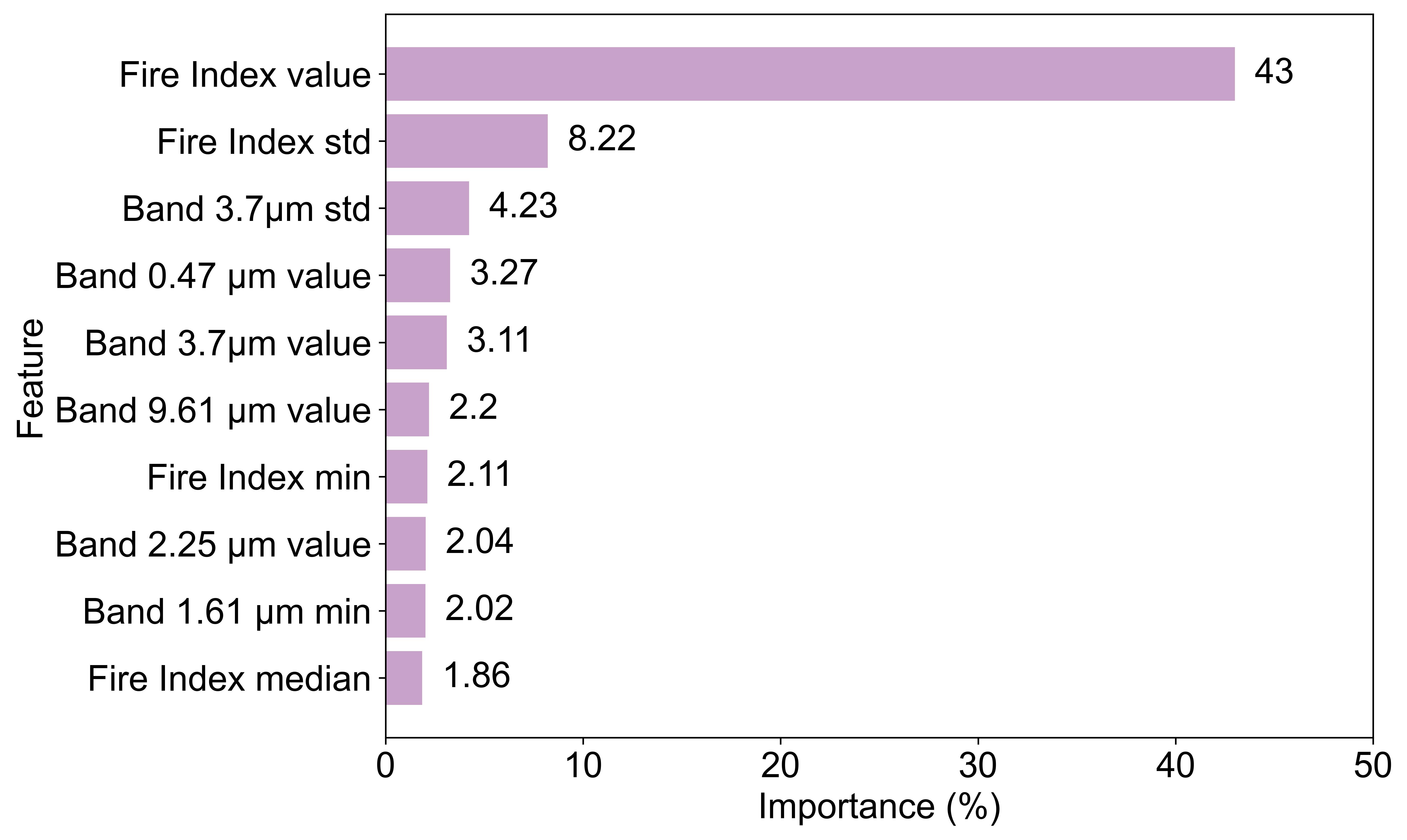
Figure B.1 shows the ten most important features in the final model. Several of the higher-ranked features come from the fire index and its statistics. This includes the fire index’s standard deviation, which incorporates information from neighboring pixels and helps the model detect local variability. Additionally, the 3.7m µm band, which is highly suitable for fire detection, demonstrated high importance. Interestingly, the 0.47m visible band also received relatively high importance. It is possible that the algorithm uses this visible band to differentiate between daytime and nighttime conditions. The figure highlights that both spectral information and simple contextual features contribute to the model’s predictions.