Collision models: Markovian and Non-Markovian impurity models

The discrete-time BLP measure only considers the system before and after applying a map $\mathcal{E}$, i.e., we wait until $U_{XY}$ (and possibly $U_{YY}$) has been fully applied before considering the system. However, this operation has a duration $\Delta t$. Let us choose units such that this duration is $1$, and assume that the map from $t$ to $t+1$ is CPTP. For $\epsilon\in(0,1)$, the map from $t$ to $t+\epsilon$ is CPTP, but in general, the map from $t+\epsilon$ to $t+1$ is not. Therefore, CP-divisibility is broken, and the trace distance of two states from $t+\epsilon$ to $t+1$ may increase. We now see that whether or not a dynamics is considered Markovian can be determined by how finely we choose to coarse-grain time.

We can consider a similar result for a Markovian impurity model. If we coarse-grain time and only consider the system for $t\in p\mathbb{N}$, then for $m\in\mathbb{N}$, we can write the map from $\rho_{X_{mp}}$ to $\rho_{X_{(m+1)p}}$ as a CPTP map $\mathcal{E}^{\prime\prime}$ given by

where $\rho^{\prime}_{Y_{m+1}}$ and $U_{XY_{(m+1)p}}$ are given by

The time dependence of the unitaries is included to clarify which ancillas they act upon. Note that the partial trace over an ancilla commutes with all operators that do not act on that ancilla, which is why we can wait to trace out all $p$ ancillas at $t=(m+1)p$. Therefore, we have shown that by coarse-graining time and considering $\bigotimes_{t=mp+1}^{(m+1)p}\rho_{Y_{t}}$ as one larger ancilla, the $p$-impurity model can be viewed as a Markovian map, i.e., the trace distance between states never increases for $t\in p\mathbb{N}$.

However, in this paper we will concern ourselves with monitored CMs where measurements are made at every time step, and hence the system must be considered for all $t\in\mathbb{N}$. Therefore, for our purposes, the map is not CP-divisible and may satisfy $\mathcal{N}_{\mathrm{BLP}}>0$ for $p\geq 2$.

In order to prove Prop. 4.1, we first show that the reduced system state is the same before and after a $YY$ interaction, as shown below:

In principle, to determine if $\mathcal{N}_{\mathrm{BLP}}>0$, we must check whether there exists any pair of initial states $\{\rho_{1,0},\rho_{2,0}\}$ and any $t$ where $\Delta D(t)>0$, i.e., where

Say we find a pair $\{\rho_{1,0},\rho_{2,0}\}$ such that $\Delta D(T)>0$, and $T=mp+k$, where $m,k\in\mathbb{N}$ and $1<k\leq p$. At the $t$th time step, where $t\in p\mathbb{N}+1$, $\rho_{X}$ is uncorrelated to the incoming ancilla ($\rho_{X_{t-1}Y_{t}}=\rho_{X_{t-1}}\otimes\rho_{Y_{t}}$). Therefore, we can take $\{\rho^{\prime}_{1,0},\rho^{\prime}_{2,0}\}=\{\rho_{1,mp},\rho_{2,mp}\}$, and we will have $\Delta D(k)>0$. Therefore, we only need to check a maximum of $p$ time steps to determine if $\mathcal{N}_{\mathrm{BLP}}>0$, assuming that we check all possible initial state pairs (or use suitable heuristics).

Now Prop. 4.1 becomes almost trivial. If a $p$-impurity model is determined to be non-Markovian, then we have found an initial pair $\{\rho_{1,0},\rho_{2,0}\}$ such that $\Delta D(k)>0$ for $1<k\leq p$. Consider passing the same pair through the $(p+1)$-impurity model (call the pair $\{\rho^{\prime}_{1,0},\rho^{\prime}_{2,0}\}$). For $t\leq p-1$, we clearly have $\{\rho^{\prime}_{1,t},\rho^{\prime}_{2,t}\}=\{\rho_{1,t},\rho_{2,t}\}$. Also, on the $p$th time step, $U_{Y_{p}Y_{p+1}}$ is a partial swap for the $(p+1)$-impurity model and effectively $\mathbb{I}$ for the $p$-impurity model, and Eq. (16) shows that $\{\rho^{\prime}_{1,p},\rho^{\prime}_{2,p}\}=\{\rho_{1,p},\rho_{2,p}\}$ still holds. Hence, for any valid $k$, the $(p+1)$-impurity model satisfies $\Delta D(k)>0$ and is therefore also non-Markovian.

A process is trivially Markovian for $p=1$. Therefore, if a process is non-Markovian for $p=\infty$, then at some finite value there was a transition from Markovian to non-Markovian. We call this value, the smallest value for which the $p$-impurity model is non-Markovian, the critical $p$, denoted as $p^{\prime}$.

In this section, we numerically investigate $p^{\prime}$ for the canonical non-Markovian CM described by Eq. (8), with $XY$ and $YY$ interactions parameterized by $\theta_{XY}$ and $\theta_{YY}$, respectively. Starting with the $1$-impurity model with no $YY$ interactions and increasing $p$, the simulations will determine if and when the model transitions to being non-Markovian, where $\mathcal{N}_{\mathrm{BLP}}$ is calculated using the $\sigma_{x}$ eigenstates as the initial state pair. We expect that increasing $\theta_{XY}$ and $\theta_{YY}$ will tend to increase $\mathcal{N}_{\mathrm{BLP}}$ and decrease $p^{\prime}$.

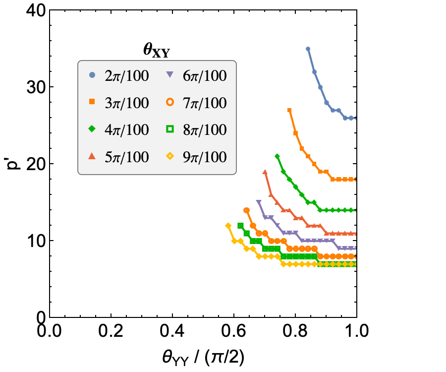
Numerical results of $p^{\prime}$ as a function of $\theta_{YY}$ for various values of $\theta_{XY}$ are shown in Fig. 3. Remember that for a specific $\theta_{XY}$ curve, on or above the line is non-Markovian ($\mathcal{N}_{\mathrm{BLP}}>0$). We can see that for small $\theta_{XY}$, $p^{\prime}$ is large, even for $\theta_{YY}\approx\pi/2$. As expected, in general for a fixed $\theta_{XY}$, decreasing $\theta_{YY}$ results in a greater $p^{\prime}$, and similarly, for a fixed $\theta_{YY}$, decreasing $\theta_{XY}$ usually results in a greater $p^{\prime}$. We also show $p^{\prime}(\theta_{XY},\theta_{YY})$ in Fig. 4 for clarity, and it is apparent that the relationship is nontrivial.

Recall that due to the discrete nature of $p$, these curves are all step functions. Also observe that, for high enough $\theta_{XY}$ and $\theta_{YY}$, even $p=2$ results in $\mathcal{N}_{\mathrm{BLP}}>0$. Additionally, it is apparent that for every value of $\theta_{XY}$, an asymptote is eventually approached when decreasing $\theta_{YY}$, and to the left of the asymptote, the process remains Markovian for all $p$ values, even when $p=\infty$, i.e., no impurities.

Note that only values of $p^{\prime}$ up to 40 were tested due to computational constraints. However, within 40 time steps, the system is in most cases very close to equilibrium, and revivals in trace distance are therefore unlikely after that. Also, when we examined values of $\theta_{YY}$ close to the asymptote by looking at 100 time steps, we observed a very quick jump from values of $p^{\prime}$ being on the order of 10 to being greater than 100 (likely infinite). Additionally, although Ref. [6] only considered a purely non-Markovian CM (effectively $p=\infty$), they observed a similar rapid asymptotic approach to $\mathcal{N}_{\mathrm{BLP}}=0$ upon decreasing $\theta_{YY}$. Hence, we can confidently say that the $p^{\prime}$ values of Fig. 4 which are greater than 40 most likely correspond to the process remaining Markovian even for $p=\infty$.

The functional relationship of the value of $\theta_{YY}$ at which the asymptote occurs, $\theta^{\prime}_{YY}(\theta_{XY})$, is shown in Fig. 5, and we can see that as $\theta_{XY}$ is increased, $\theta^{\prime}_{YY}$ generally decreases. This results in a downward and to the left shift of the $p^{\prime}$ curves of Fig. 3 as $\theta_{XY}$ is increased.

Observe that at higher values of $\theta_{XY}$, there is a complex interplay between correlations, changes to environmental states, and the rate of approach to equilibrium. Strange phenomena can occur, such as increasing $p^{\prime}$ upon increasing $\theta_{YY}$ (see Fig. 4) or increasing $\theta^{\prime}_{YY}$ upon increasing $\theta_{XY}$ (see Fig. 5).

References

- [1] (2022) Quantum collision models: Open system dynamics from repeated interactions. Physics Reports 954, pp. 1–70. External Links: ISSN 0370-1573, Link, Document Cited by: §1, §3.1.
- [2] (2012) Open Quantum Systems: An Introduction. Springer Berlin Heidelberg. External Links: ISBN 9783642233548, ISSN 2191-5431, Link, Document Cited by: §2.
- [3] (2009) Measure for the Degree of Non-Markovian Behavior of Quantum Processes in Open Systems. Physical Review Letters 103 (21). External Links: ISSN 1079-7114, Link, Document Cited by: §3.
- [4] (1975) Completely Positive Maps and Entropy Inequalities. Communications in Mathematical Physics 40, pp. 147–151. External Links: Document Cited by: §3.
- [5] (2022) Entropy Production in Non-Markovian Collision Models: Information Backflow vs. System-Environment Correlations. Entropy 24 (6), pp. 824. External Links: ISSN 1099-4300, Link, Document Cited by: §3.1.
- [6] (2026) Nonequilibrium steady states in multibath quantum collision models. Physical Review A 113 (2). External Links: ISSN 2469-9934, Link, Document Cited by: §4.1.3.